An Ontology-Based Framework for Geospatial Integration and Querying of Raster Data Cube Using Virtual Knowledge Graphs

Abstract

The integration of the raster data cube alongside another form of geospatial data (e.g., vector data) raises considerable challenges when it comes to managing and representing it using knowledge graphs. Such integration can play an invaluable role in handling the heterogeneity of geospatial data and linking the raster data cube to semantic technology standards. Many recent approaches have been attempted to address this issue, but they often lack robust formal elaboration or solely concentrate on integrating raster data cubes without considering the inclusion of semantic spatial entities along with their spatial relationships. This may constitute a major shortcoming when it comes to performing advanced geospatial queries and semantically enriching geospatial models. In this paper, we propose a framework that can enable such semantic integration and advanced querying of raster data cubes based on the virtual knowledge graph (VKG) paradigm. This framework defines a semantic representation model for raster data cubes that extends the GeoSPARQL ontology. With such a model, we can combine the semantics of raster data cubes with features-based models that involve geometries as well as spatial and topological relationships. This could allow us to formulate spatiotemporal queries using SPARQL in a natural way by using ontological concepts at an appropriate level of abstraction. We propose an implementation of the proposed framework based on a VKG system architecture. In addition, we perform an experimental evaluation to compare our framework with other existing systems in terms of performance and scalability. Finally, we show the potential and the limitations of our implementation and we discuss several possible future works.

1. Introduction

Recent advances in geospatial data acquisition, particularly in the areas of remote sensing as well as positioning and communication technologies, have led to the accumulation of an enormous amount of geospatial data with temporal properties. One widely used spatiotemporal data structure is the raster data cube, which describes the continuous distribution of a variable in space and its change over time. It can be seen as a special case of a multi-dimensional array with three dimensions: two spatial and one temporal [1,2]. Such a form of spatiotemporal data (i.e., a data cube) raises considerable challenges when it comes to managing and portraying it using a knowledge graph. The smart integration of data cubes using knowledge graphs can play an invaluable role in handling the heterogeneity of geospatial data and linking them with other enhanced semantics and knowledge. Knowledge graphs manage data and knowledge in the form of a semantic directed graph that allows the capture of relationships between instances of different concepts and offers a quite flexible structure compared to the relational structure [3]. In addition, its reasoning capabilities can facilitate the inference of more implicit facts and knowledge, and most importantly, it can verify the consistency of the data/knowledge as a whole, which can contribute to the intelligent integration of different data sources and forms.

Many thoughtful and recent approaches have been tried to address the representation of raster data cubes using knowledge graphs [4,5,6]. However, these solutions are not yet mature. They either lack strong formal development or focus only on the management of this form (i.e., a raster data cube) without combining it with other data forms that represent discrete space with a set of spatial features along with their spatial relationships. This can present a major shortcoming when it comes to performing advanced geospatial queries and semantically enriching geospatial models. One feasible solution would be to translate the raster data cubes into a linked dataset (i.e., a set of RDF triples), manage them using a knowledge graph, and then combine them with other geospatial knowledge graphs to perform more advanced geospatial queries [7,8,9]. However, such a solution implies the materialization of the data into RDF triples. This directly leads to unnecessary high redundancy, and then high storage costs and scalability issues when the data size increases. One alternative approach to avoiding materialization is to use an ontology to define a semantic layer of the data cube and link it to the data source through mapping. Thereafter, and only during the query process, the raster knowledge graph (i.e., the RDF triples representing the raster data cubes) could be generated. This virtual knowledge graph (VKG) [10] seems to be promising to link different forms of geospatial data and manage spatiotemporal semantics at a high level of abstraction, which could significantly reduce the high redundancy that materialization would entail.

In this paper, we propose a framework that can enable such semantic integration and advanced querying of raster data cubes based on VKG. We define a semantic representation model for raster data cubes in this framework by extending the GeoSPARQL ontology. With such a model, we can combine the semantics of raster data cubes with a vector data model that represents features using geometries and attributes. We propose an implementation of our framework and confront it with a set of scenarios that take the form of basic and advanced semantic geospatial queries. With this implementation, one can formulate spatiotemporal queries using SPARQL in a natural way by using ontological concepts at an appropriate level of abstraction. We then perform an experimental evaluation to compare our framework with other existing systems in terms of performance and scalability and show the potential as well as the limitations of our implementation.

The rest of the paper is organized as follows. Section 2 explores the literature regarding the integration of raster data cubes and their link to knowledge graphs and summarizes the different approaches that address this issue. Section 3 explains our proposed framework at the conceptual level by proposing a semantic representation model as well as a taxonomy of semantic geospatial queries. Section 4 presents the implementation aspect of the proposed framework and how, concretely, the raster data cube could be linked virtually to the knowledge graphs with an appropriate architecture and data modeling process. Section 5 evaluates the semantic query capability of our implemented framework by proposing a use case with its datasets, and formulating basic and advanced geospatial queries using SPARQL. In addition, this section evaluates the query performance of our approach and makes a comparison with other systems. Finally, Section 6 concludes the results, highlighting the advantages and disadvantages of our framework, and then provides insights for future work.

2. Related Works

The smart integration of earth observation (EO) raster data cubes has been extensively investigated from multiple aspects. While many works have focused on providing an accurate formalization and algebra to properly represent and manipulate this concept, considering it a special case of multidimensional arrays [1,2], other works have focused on effective processing and analyzing raster data cubes. These works started with the proposal of array database systems such as SciDB [11] or Rasdaman [12], up to the development of an appropriate advanced infrastructure capable of supporting such a task with high performance and appropriate scalability on a large amount of data [13,14,15,16].

Further solutions have been proposed to facilitate the efficient integration and querying of raster data cubes. One of the most important advancements in this area was the creation of the Web Coverage Processing Service (WCPS) [17]. This standard enhances and expands the basic access to geospatial raster coverage data by providing a web interface in the form of a retrieval language that can handle on-the-fly processing and filtering of multi-dimensional raster coverages. It also enables the execution of more complex queries. The Open Geospatial Consortium (OGC) has been responsible for maintaining this language, and it has been further improved by the Petascope implementation of WCPS [18]. This implementation enables the translation of queries from the aforementioned language into Rasdaman array DBMS queries. However, despite the existence of such powerful solutions, there has not been coupling between raster data cubes and conventional linked data technologies.

Several efforts were initiated to address such a coupling, starting first at the conceptual level by proposing a semantic model in the form of ontologies to capture the data cube properties. The main efforts culminated in the proposal of the RDF Data Cube (QB) ontology by the World Wide Web Consortium (W3C) in 2017 [19]. This ontology was originally conceived to handle multi-dimensional statistical data, and subsequently adopted for representing Earth Observation (EO) data that are conceived as a data cube with the three dimensions of latitude, longitude, and time. The main benefit of QB ontology emanates from the combination of several standard vocabularies, such as Simple Knowledge Organization System (SKOS), sensor network (SSN), OWL-time, and Provenance Ontology (PROV-O) [19]. An auxiliary ontology designated as the RDF Data Cube extensions for spatiotemporal components (QB4ST), was meticulously formulated by the W3C [20]. The objective was to enable a flexible adaptation of data cubes to various dimensions, with particular emphasis on spatiotemporal aspects, allowing the formation of support coverage that encompasses dimensions ranging from one to four [21]. Nevertheless, despite the importance of these conceptual efforts, they have not been able to address implementation considerations regarding the efficient querying of Earth Observation (EO) data using SPARQL. In contrast, other initiatives have focused more on this facet of implementation, resulting in two main solutions, namely SciSPARQL [4,22] and GeoSPARQL+ [23]. The goal of these solutions was to provide SPARQL support for scientific array data and raster coverages by defining new data types, algebras, and operators for raster arrays. While these solutions offered computational benefits, they only considered the static aspect of raster coverags and did not adequately handle the temporal dimension. Furthermore, users needed to familiarize themselves with a set of new raster data operators, in addition to the underlying SPARQL syntax, in order to perform geospatial queries.

Several approaches have been proposed to achieve the integration of raster data cubes, including their temporal dimension, while establishing connections with knowledge graph and semantic web technologies. These approaches can be categorized into three main types. The first approach focuses on feature-based representation, placing emphasis on the selection or derivation of ontological features through the aggregation of multiple raster cells. Subsequently, instead of querying and analyzing the data cubes as a whole, the system directly queries these specific features that emerge as abstractions of the underlying data [24,25,26]. This approach has been significantly enhanced by the research conducted by [9,27], which proposed a semantic and configurable extract, transform, load (ETL) mechanism. This ETL process serves as a pipeline responsible for extracting raster cells, recognized as observations, and establishing associations with geometric entities denoted as territorial units. However, despite the significance of this work, a rigorous formalism and representation for the semantic model, as well as the mapping process between datasets and ontological features, are still lacking.

The second type of approach has centered on converting the entire geospatial dataset into the RDF data format and then storing and managing it in a spatial database. One of the main systems developed for this purpose was Strabon [28]. Strabon has been extended to be able to manage and query spatiotemporal data, and more particularly, time-stamped satellite images in their RDF format [7]. Upon that, and to assist in the translation between common geospatial formats and linked data, an open-source tool was developed to facilitate this task [8]. The main advantage of this approach is that the integrated data are gathered from a unified source; thus, the process of rewriting queries is not necessary, and the processing of queries is both centralized and prompt. However, these materialized approaches have major drawbacks, including the necessity of extra storage since the data are replicated, which implies an added storage cost as well as a maintenance cost. In addition, materialized data can quickly become stale if the data source is frequently updated.

The third approach consists of virtually linking a knowledge graph to data cubes without materializing it in the form of a set of RDF triples. Such an approach is essentially based on the virtual knowledge graph (VKG) paradigm, also known as an OBDA (ontology-based data access) [29,30,31]. A VKG consists of three main components: (1) a collection of data sources, (2) an ontology, and (3) mapping between the two. The ontology provides a high-level specification of the domain of interest and is semantically linked to the data sources by a mapping consisting of a series of mapping statements, where the standard mapping language is R2RML [32]. The ontology and mapping, called the VKG specification, expose the underlying data sources as a virtual RDF graph that can be accessed at query time using the standard W3C SPARQL language. When the user expresses SPARQL queries, the VKG system, e.g., Ontop [33], translates these queries into ones that are directly evaluated by the underlying database engine (e.g., SQL) without having to convert and materialize the original data into RDF and then store them in a triple store. The VKG system Ontop has implemented most of the GeoSPARQL functions [10] elaborated by the Open Geospatial Consortium (OGC), which is specifically designed as a geographic query language that extends SPARQL [34]. Using VKG, one can perform geospatial queries on relational data sources to query features, geometries, attributes, and their topological relationships using SPARQL [35,36]. Additional efforts have been made to manage knowledge consistency when querying geospatial data through VKG [37]. Also, work has been performed to show the potential of VKG to support some spatial–temporal data queries [38]. However, no work has been carried out on harnessing VKG to properly integrate and query raster data cubes.

Another solution aligned with the third approach involved the creation of a knowledge hypergraph system known as Onto-KIT, which aimed to integrate and manage raster data cubes with their heterogeneous formats [5,39]. This model presents a promising approach, as a hypergraph structure encompasses a generalization of the conventional graph, allowing edges to connect more than two nodes. Leveraging the hypergraph-based model enables the integration and semantic linking of data from multiple sources, facilitating enhanced information extraction in terms of relationship abundance. The hypergraph structure serves the dual purpose of representing the semantic model and virtually managing the population process. Notably, Onto-KIT incorporates a query processing engine based on hypergraphs, enabling the efficient rewriting and execution of fundamental geospatial queries on raster data cubes.

Another notable solution in the third category is the development of GeoLD, a system that offers a dedicated GeoSPARQL query engine to handle queries involving raster data cubes [6]. This system leverages the Rasdaman array database for efficient data storage and utilizes the Petascope implementation of WCPS to facilitate web access. To establish mapping between the ontological domain and the dataset, a novel mapping process called Coverage to RDF (C2RML) is proposed, wherein the conceptual model extends the GeoSPARQL feature class with the coverage class. The system also incorporates a query engine that efficiently processes and rewrites the geospatial components of the SPARQL query into the WCPS language. The request is then transformed into the Rasdaman query language (Rasql) and executed on the Rasdaman system to obtain the desired data output. Through the mapping process, the entities in the ontological coverage model are populated, and the result is returned as an RDF dataset. One considerable advantage of this system is that it does not introduce a new collection of data operators to the SPARQL syntax, thus making it more accessible for regular SPARQL users to conduct geospatial queries on data cubes. Additionally, GeoLD demonstrates remarkable performance in executing spatiotemporal queries on data cubes, outperforming other systems like Geospark+ or Strabon. However, it should be noted that the system currently lacks the capability to perform aggregation operations, which are crucial in the geospatial query process, necessitating further development in this aspect.

Despite the valuable capabilities offered by both Onto-KIT and GeoLD, they have been limited to querying raster data cubes without supporting their combination with vector features along with their relationships. Such a combination would greatly improve the integration and semantics of geospatial querying.

In this work, we will rely on the virtual knowledge graph (VKG) paradigm as the foundation for proposing a comprehensive framework that facilitates the seamless integration of raster data cubes. Our objective is to investigate the potential of this approach (i.e., VKG) and evaluate its capacity to handle a diverse range of queries. These queries aim to retrieve information from the data cube while simultaneously combining it with another semantic layer, specifically feature-based semantics. This integration would enable the formulation of spatiotemporal queries in a more intuitive manner, leveraging ontological concepts at an appropriate level of abstraction. By exploring the limits of the VKG approach, we aim to demonstrate its efficacy in addressing the challenges associated with geospatial querying and enhancing the overall integration of raster data cubes.

3. An Ontology-Based Framework for Integrating Raster Data Cubes

In this section, we explain the conceptual aspects of our proposed framework. This mainly includes the modeling process that led us to the ontological representation of a semantic raster data cube using virtual graph knowledge.

In our ontological representation, we have chosen to rely on and use the GeoSPARQL standard only instead of reusing the data cube RDF (QB) ontology. The reason for adopting this approach is that QB, when used to represent raster data cubes, employs the concept of coverage as its basic element. This concept of coverage consists of a numerical array characterized by its spatial and temporal dimensions. However, the current landscape of OBDA systems is limited in its ability to handle spatiotemporal queries that involve combining raster data cubes with geometric features. Adopting such a coverage model by OBDA systems requires the development of new operators and functions adapted to the processing of raster data cubes and the realization of adding geometries to support such spatial-temporal queries.

In our framework, we introduce a semantic representation approach for raster data cubes. This approach is based on the concept of a spatiotemporal entity or location that encapsulates the spatial and temporal dimensions of the geospatial data cube concept. Although data cubes can possess multiple dimensions (i.e., n-dimensional), in the context of Earth observation they are often simplified to a three-dimensional model (x, y, t) or may also be a four-dimensional model known as a voxel data cube (x, y, z, t) [40]. Within our ontology, we label this spatiotemporal entity SpaceTimeLocation, and its dimensions can be adjusted based on the specific data cube type under consideration. For our focus, we narrowed the selection down to the most prevalent and simplified form of data cube, which is the three-dimensional raster data cube. The spatial aspect of the SpaceTimeLocation is acquired from the GeoSPARQL feature class for spatial reference. As for the temporal dimension, we adopt a straightforward linear time model with a single dimension. If required, the temporal dimension can be further extended to support a more complex model of time (cyclic time, relative time, temporal relations, …, etc.) by establishing connections between the SpaceTimeLocation concept and the OWL-time ontology. However, this is not within the interest or scope of this paper. The advantage of such a semantic representation is its seamless alignment with a large number of OBDA systems that offer GeoSPARQL-compliant functionalities and operations.

Additionally, with such a semantic representation, we would be able to formulate semantic geospatial queries that could combine discrete entities (i.e., features) with the properties of the continuous space represented by the data cube construct. For the modeling, we use the description logic, and at the same time, we combine it with the notation of other web semantics standards like RDF, RDFS, and  GeoSPARQL. In addition, this framework includes a taxonomy of semantic geospatial queries.

3.1. Semantic Representation of Discrete Space

We consider our discrete space as a set of geospatial entities (i.e., features) associated with their geometries and forming spatial relationships between them. We model such a space as the quadruplet:

$$\begin{array}{c}\hfill <E,T_y,S_R,F_g>where:\end{array}$$

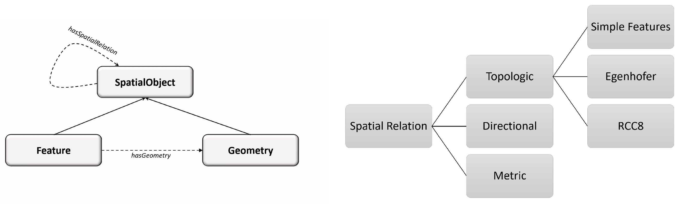
• E represents the set of entities (i.e., features) that exist in the space and that inherit all their properties from the $Feature$ class of the GeoSPARQL ontology (see Figure 1(left)), such as $E⊑Feature$;
• $T_y$ is a function that assigns to each entity $e\in E$ its type, which we denote by the function: $T_y:e⟼type$. This function corresponds to the RDF property rdf:type. In this case, we try to simplify the model by assigning a unique type to each entity instance.
• $S_R$ consists of the set of spatial relations that can link two spatial entities, $e_1$ and $e_2$, where $S_R\subseteq E\times E$. This spatial relation could be metric, directional, or topological (see Figure 1(right)). For the taxonomy of the topological relations between two entities, we adopt the one used by the GeoSPARQL standard (see

  Table 1. Different topological function classifications implemented by GeoSPARQL standard [34].

  OGC	Egenhofer	RCC8
  geo:sfEquals	geo:ehEquals	geo:rcc8eq
  geo:sfDisjoint	geo:ehDisjoint	geo:rcc8dc
  geo:sfIntersects	geo:ehMeet	geo:rcc8ec
  geo:sfTouches	geo:ehOverlap	geo:rcc8po
  geo:sfWithin	geo:ehCoveredBy	geo:rcc8tppi
  geo:sfContains	geo:ehContains	geo:rcc8tpp
  geo:sfOverlaps	geo:ehInside	geo:rcc8ntpp
  geo:sfCrosses	geo:ehCovers	geo:rcc8ntppi

  ).
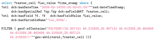
• Finally, $F_g$ is a function that assigns for each entity $e\in E$ its geometrical representation, where $F_g:E\to G$. This function corresponds to the GeoSPARQL property $geo:hasGeometry$, where $G⊑geo:Geometry$. We adopt the same taxonomy as the GeoSPARQL standard for this class, which is by default in compliance with OGC standards (see Figure 2).

3.2. Semantic Representation of Continuous Space

Within a continuous space, a potentially infinite number of spatially distributed properties (e.g., temperature, pressure, humidity, etc.) can be identified at each location in that space. A location in geographic space can be determined using a two-dimensional coordinate system, represented by (x, y) coordinates, or a three-dimensional coordinate system, represented by (x, y, z) coordinates. Another alternative is to use geographic coordinates, which include latitude and longitude values, rather than projected coordinates. The relationship or association between a location and its property’s value is represented in the form of a function called a field [41,42]. A field can be seen as a set of observations where each one has been measured and associated with a geo-referenced component.

In this section, we use the definition of the spatiotemporal field that has been developed in the works [43,44] and subsequently further specify it to yield a basic definition of the notion of a data cube, and finally propose an ontological model to capture the domain of the semantic data cube.

3.2.1. Definition of Spatiotemporal Field

In the works [43,44], the notion of the spatiotemporal field was defined as a function f:

$$\begin{array}{c}\hfill f:S\times T\to \mathcal{P}\left(H\right)where\end{array}$$

• $S\times T$ consists of a spatiotemporal domain, such that S consists of a set of locations in geographic space that we denote as spatial atoms, and T is an ordered domain consisting of a sequence of timestamps: $T=\{t_1,t_2,\dots ,t_k,\dots ,t_n\}$.
• H consists of a set of property-value pairs $(M,V)$, such that M is a set of properties and V is the set of numerical values associated with the property M. $\mathcal{P}\left(H\right)$ represents the set of all subsets of H (i.e., the power set), which consists of the range of the field f.

The function f assigns for each spatiotemporal location $l\in L$ a subset of property-value pairs $(m,v)\in M\times V$. This function will help us define the notion of the data cube by adding constraints to its domain.

3.2.2. Basic Definition of Data Cube

In our case, we use the previous definition in order to define the notion of the data cube. This notion is defined as a triplet as follows:

$$\begin{array}{c}\hfill F_L=(S\times T,f,\mathcal{P}\left(H\right))\end{array}$$

We consider the notion of a data cube as a special case of the spatiotemporal field f applying three constraints, which we express precisely as follows:

• S consists of a set of sampled spatial atoms within a given spatial coverage. Each spatial atom $s\in S$ is bidimensionally indexed by the indices $(i,j)\in (m,p)$, where m and p respectively denote the number of rows and columns. This uniform sample S is maintained across all timestamps $t_k$ where every space–time location $(s_i{}_{,}{}_j,t_k)$ has one and only one value from the range of the function f:

  $$\begin{array}{c}\hfill \forall s_i{}_{,}{}_j\in S,\forall t_k\in T\exists !h\in \mathcal{P}\left(H\right)suchthatf(s_i{}_{,}{}_j,t_k)=h\end{array}$$
• All time elements $t_k\in T$ are temporally regular, which means that the temporal distance between each two consecutive times $t_k$ and $t_{k+1}$ corresponds to the duration constant ${\delta }_t>0$. This constant is designated as the temporal resolution of a data cube.

  $$\begin{array}{c}\hfill \forall t_k,t_{k_{+}1}\in T:(t_k{}_{+}{}_1-t_k)={\delta }_t\end{array}$$
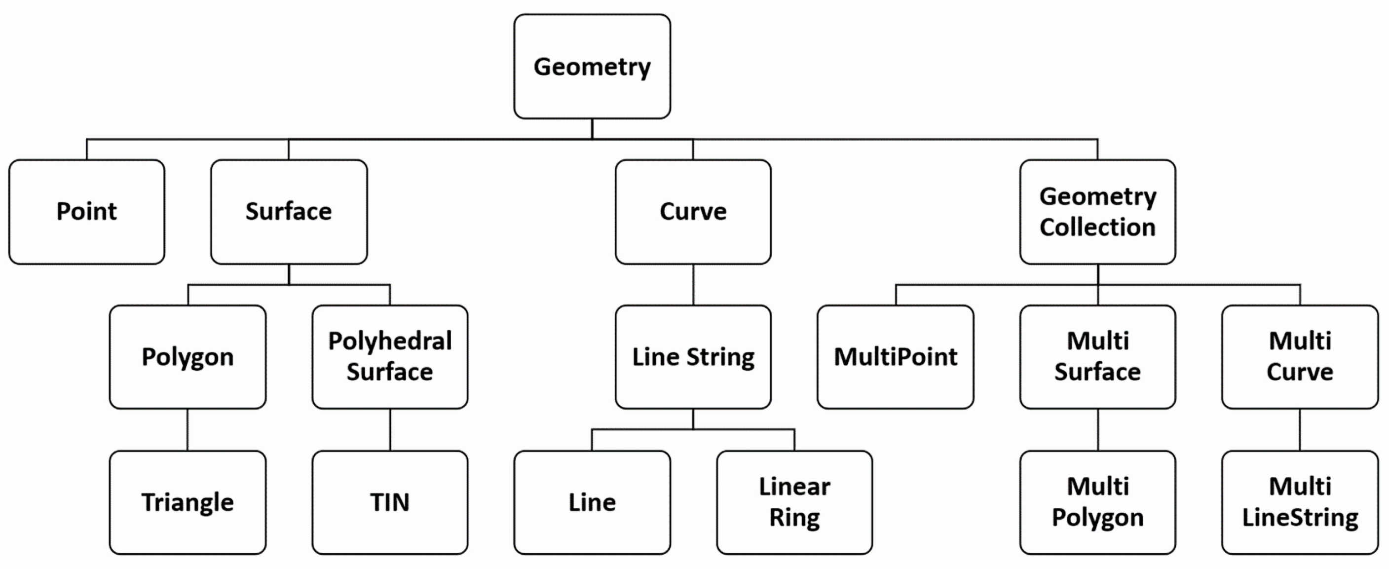
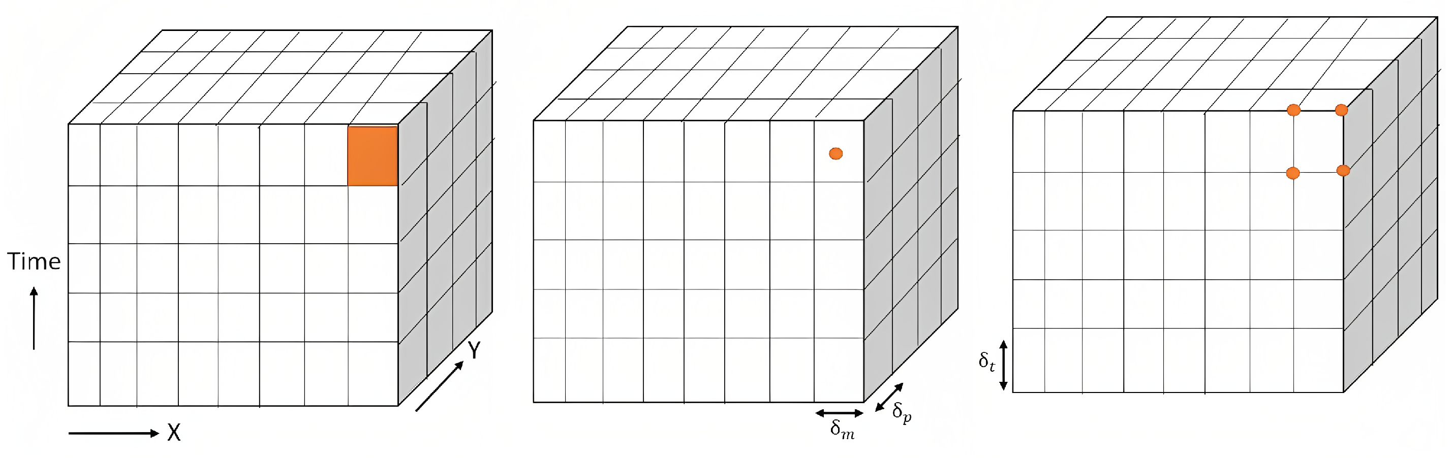
• The spatial atom $s\in S$ of a raster data cube could have many abstractions (i.e., spatial representation). As shown in Figure 3, a spatial atom can be either abstracted as a rectangle or as a point (excluding the center or the left/top corner of a rectangular raster cell). The spatial atoms in the raster data cube must be spatially regular, which means the size and shape of these spatial atoms (i.e., cells) should be consistent across the entire raster data cube coverage, forming a regular grid pattern. Additionally, the spatial arrangement and spacing between adjacent spatial atoms should be constant throughout the entire dataset.

In the case where the spatial atoms are abstracted as points, spatial regularity implies that vertically and horizontally, the contiguous spatial atoms are separated by the same consecutive distances ${\delta }_m>0$ and ${\delta }_p>0$. We express this constraint as follows:

$$\begin{array}{c}\hfill \forall s_i{}_{,}{}_j,s_i{}_{,}{}_j{}_{+}{}_1,s_i{}_{+}{}_1{}_{,}{}_j:(s_i{}_{,}{}_j{}_{+}{}_1-s_i{}_{,}{}_j)={\delta }_{p}and(s_i{}_{+}{}_1{}_{,}{}_j-s_i{}_{,}{}_j)={\delta }_m\end{array}$$

The pair $({\delta }_m,{\delta }_p)$ is designated as the spatial resolution of a data cube.

3.2.3. An Ontological Representation of Raster Data Cube

We propose an ontology in order to capture the key concepts along with their relationships and constraints pertaining to the notion of a semantic data cube. For this purpose, we employ description logic (DL), which is considered a fragment of first-order logic and serves as the formal expressive language of the ontological web language (OWL2). Using the expressiveness of DL, we formulate the set of axioms that bind higher-level concepts as well as the set of properties (i.e., roles) that would capture the notion of a semantic data cube. To do so, three main concepts that were evoked in the basic definition of a data cube will be semantically defined using DL, especially the main concepts $S\times T$, f, and $\mathcal{P}\left(H\right)$.

Initially, we need to define the atomic concepts that constitute the building blocks on which our axioms will be based. The first concept consists of the spatial domain of any raster data cube. We represent this concept with the class dcb:FieldAtom, which is defined as the union of the classes geo:Point and geo:Polygon. This class refers to the set S defined in the previous section.

$$\begin{array}{c}\hfill FieldAtom\equiv Point\bigsqcup Polygon\end{array}$$

In this definition, we assume that any spatial atom of a data cube could be represented either by a polygon, where a rectangle or a square is a special case of it, or by a point, which could represent the center or the left/right corner of each spatial atom of a data cube. The second concept consists of representing the set of all variable names (e.g., temperature, rainfall, humidity, etc.) with the class dcb:FieldPropertyVar. This class refers to the set M defined in Section 3.2. The third concept consists of the set of all values V that could be affected by the spatial atoms of a data cube. Often these values are of the numeric type and sometimes textual (e.g., a data cube that represents the variable of landcover types). However, since there is no need to restrict these values to only these types, we prefer to remain generic and represent the class dcb:Value as equivalent to the related generic type rdfs:Literal, which represents all data types in the system.

$$\begin{array}{c}\hfill Value\equiv rdfs:Literal\end{array}$$

The last concept consists of the time T, which we represent simply using the data property DateTimestamp, which represents the set of ordered instants.

The second step entails the derivation of key concepts by compounding the atomic ones and specifying the set of axioms that can be applied to any semantic data cube.

In the previous section, we considered that a spatial atom in a data cube could be associated with one or a collection (i.e., a subset) of property-value pairs. This subset was represented by the set $H=(M,V)$. This leads us to represent the first key concept, which consists of the class dcb:FieldPropValue as follows:

$$\begin{array}{c}\begin{array}{c}{\displaystyle FieldPropValue⊑=1hasFieldProp.FieldPropertyVar\sqcap }\hfill \\ {\displaystyle =1hasFieldValue.Value}\hfill \end{array}\end{array}$$

The class dcb:FieldPropValue is subsumed by the intersections of two classes $=1hasFieldProp.FieldPropertyVar$ and $=1hasFieldValue.Value$ where the former refers to all instances having exactly one relationship dcb:hasFieldProp with the class dcb:FieldPropertyVar and the latter refers to all instances having exactly one relationship dcb:hasFieldValue with the class dcb:Value. In other words, this description implies that each instance of the dcb:FieldPropValue class is composed of a unique pair made up of an instance of the dcb:FieldProperty class together with an instance of the dcb:Value class. The second key concept consists of defining the spatiotemporal domain ($S\times T$) related to a semantic data cube, which is represented with the class dcb:SpaceTimeLocation and the following axiom:

$$\begin{array}{c}\begin{array}{c}{\displaystyle SpaceTimeLocation\equiv \exists hasSpatialRef.FieldAtom\sqcap }\hfill \\ {\displaystyle \exists hasTemporalRef.TimeStamp\sqcap }\hfill \\ \forall hasField.FieldPropValue\hfill \end{array}\end{array}$$

In this axiom, we define the class dcb:SpaceTimeLocation as an equivalence of the intersection of three classes: the $\exists hasSpatialRef.FieldAtom$, which starts with the existential quantifier ∃ that denotes the set of all instances connected to the class dcb:FieldAtom through the relation dcb:hasSpatialRef. The class $\exists hasTemporalRef.TimeStamp$, for which the same case applies and which denotes the set of all instances connected to the data type TimeStamp through the relation dcb:hasTemporalRef. And the third class, $\forall hasField.FieldPropValue$, which starts with the universal quantifier ∀, defines the set of all instances that have only been connected to the class dcb:FieldPropValue through the relationship dcb:hasField. This means that any instance that is a subject of the dcb:hasField property must necessarily be connected to the instance of the dcb:FieldPropValue class. However, such a definition does not necessarily imply that every instance of dcb:SpaceTimeLocation must be associated with an instance of the class dcb:FieldPropValue. In other words, for an instance to stand for a space–time location, it must at least be related to a spatial atom (i.e., a cell) represented by the dcb:FieldAtom class and have at least one temporal reference represented by the TimeStamp data type. Even if such a space–time location is not associated with a property-value pair, it is nevertheless still considered an instance of the dcb:SpaceTimeLocation class.

This last point leads us to define the notion of observation and to clearly differentiate it from the notion of spatiotemporal location. Thus, an observation could be seen as a subclass of dcb:SpaceTimeLocation with an obligation to be involved in the dcb:hasField relation along with the dcb:FieldPropValue class. In this case, we formulate this axiom as follows, using the intersection of two classes:

$$\begin{array}{c}\begin{array}{c}{\displaystyle Observation\equiv SpaceTimeLocation\sqcap }\hfill \\ {\displaystyle \exists hasField.FieldPropValue}\hfill \end{array}\end{array}$$

This implies that an observation must possess spatial and temporal references, and furthermore, it must be associated with at least one property-value pair that is an instance of the class dcb:FieldPropValue and this is necessarily through the relation dcb:hasField. This relationship represents the most important association that plays the role of linking the spatiotemporal domain of a data cube with its range. Precisely, this relation dcb:hasField represents the function f, which is considered the definition of the spatiotemporal field in the previous section. For this reason, we chose to give a definition of this relationship as follows:

$$\begin{array}{c}\hfill \begin{array}{c}{\displaystyle \exists hasField.\top ⊑\le 1SpaceTimeLocation}\hfill \\ {\displaystyle \top ⊑\forall hasField.FieldPropValue}\hfill \end{array}\end{array}$$

The relationship dcb:hasField has as its domain the class dcb:SpaceTimeLocation and exclusively as its range the class dcb:FieldPropValue. Since there are no cardinality restrictions on the range of dcb:hasField, an instance of dcb:SpaceTimeLocation can have from zero to multiple instances related to the dcb:FieldPropValue class. This means that a space–time location might have a collection of property-value pairs. This last point was expressed in the previous section using the range of the function f, which is denoted by the power set $\mathcal{P}\left(H\right)$.

On the other hand, the existence of the cardinality notation $\le 1$ in the domain of the function dcb:hasField implies that this relation is inversely functional. This implies that each instance of the range related to the dcb:hasField relation can be associated with at most one spatiotemporal location. Such a characteristic leads us to specify the inverse function related to the dcb:hasField relation that we call hasSTL.

$$\begin{array}{c}\hfill hasSTL\equiv hasFiel{d}^{-}\end{array}$$

This relation would therefore be functional and would allow one to easily find, for each instance of the class dcb:FieldPropValue, at most one associated instance of the dcb:SpaceTimeLocation class.

The last concept and axiom related to the design of our ontology concerns the notion of a data cube and how it is defined in relation to the other concepts. In this model, a data cube concept is a subclass of the intersection of three anonymous classes:

$$\begin{array}{c}\hfill \begin{array}{c}{\displaystyle DataCube⊑=1hasCoverageParams.CoverageParams\sqcap }\hfill \\ {\displaystyle \exists hasPropSet.FieldPropertyVar\sqcap }\hfill \\ =1hasTimeExtent.TimeExtent\hfill \end{array}\end{array}$$

• An instance of the dcb:DataCube class must first be associated with one and only one instance of the dcb:CoverageParams class. This class defines the main spatial and temporal parameters that shape the spatiotemporal domain of a semantic data cube. It defines exactly its spatial resolution (i.e., $({\delta }_m,{\delta }_p)$) as well as its temporal resolution (i.e., ${\delta }_t$) and the coordinates of the point that constitutes the left corner of the data cube. With these parameters, we will be able to reconstruct the spatiotemporal domain of any given dcb:DataCube instance.
• Each instance of dcb:DataCube records the values of one or more distributed variables (e.g., temperature, evapotranspiration, cloud cover, etc.). Thus, for each instance of the dcb:DataCube class, there must be a relationship with at least one instance of the dcb:FieldPropertyVar class. This last class represents the set of all the distributed variables. Thus, the relation between the class dcb:DataCube and the other classes of our ontology is materialized by its relation to the class dcb:FieldPropertyVar through the relation dcb:hasPropSet.
• Any instance of the dcb:DataCube class embodies a unique temporal extent for which it holds. The temporal extent signifies the valid time interval between when the data cube starts recording its values and the end of that recording. Similarly to the constraint in the dcb:CoverageParams class, each instance of dcb:DataCube must possess only one and only one temporal extent.

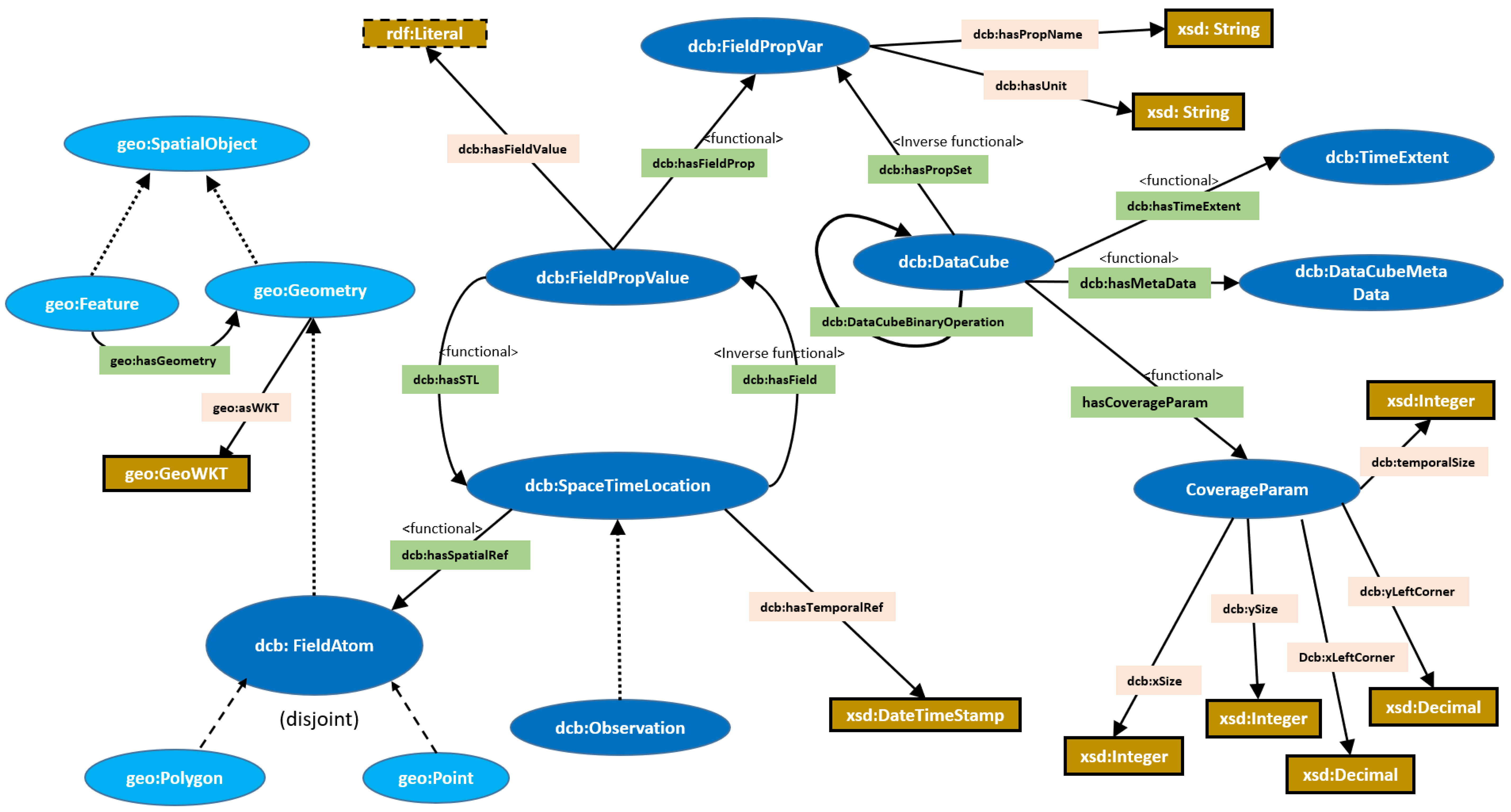
Another property that could potentially be assigned to the dcb:DataCube class is the abstract relation dcb:DataCubeBinaryRelation which could specifically represent the set of topological and arithmetic operations between each pair of two instances of the dcb:DataCube class. A dcb:DataCube class can also be associated with a class that stores all of its metadata, which may include the type of sensors used, the owner of such data, and others. The design of the whole ontology, which mentions the characteristics of data cubes and their relationships with all other classes, is illustrated in Figure 4.

3.3. Ontology-Based Geospatial Queries

To evaluate the expressivity of the proposed semantic representation model, we carefully designed a set of geospatial queries. These queries can be classified into a taxonomy that captures most of their aspects. Thus, we present a taxonomy within which each query can find its semantic position. We then take a sample of scenarios and classify them according to this taxonomy.

3.3.1. Taxonomy of Semantic Geospatial Queries

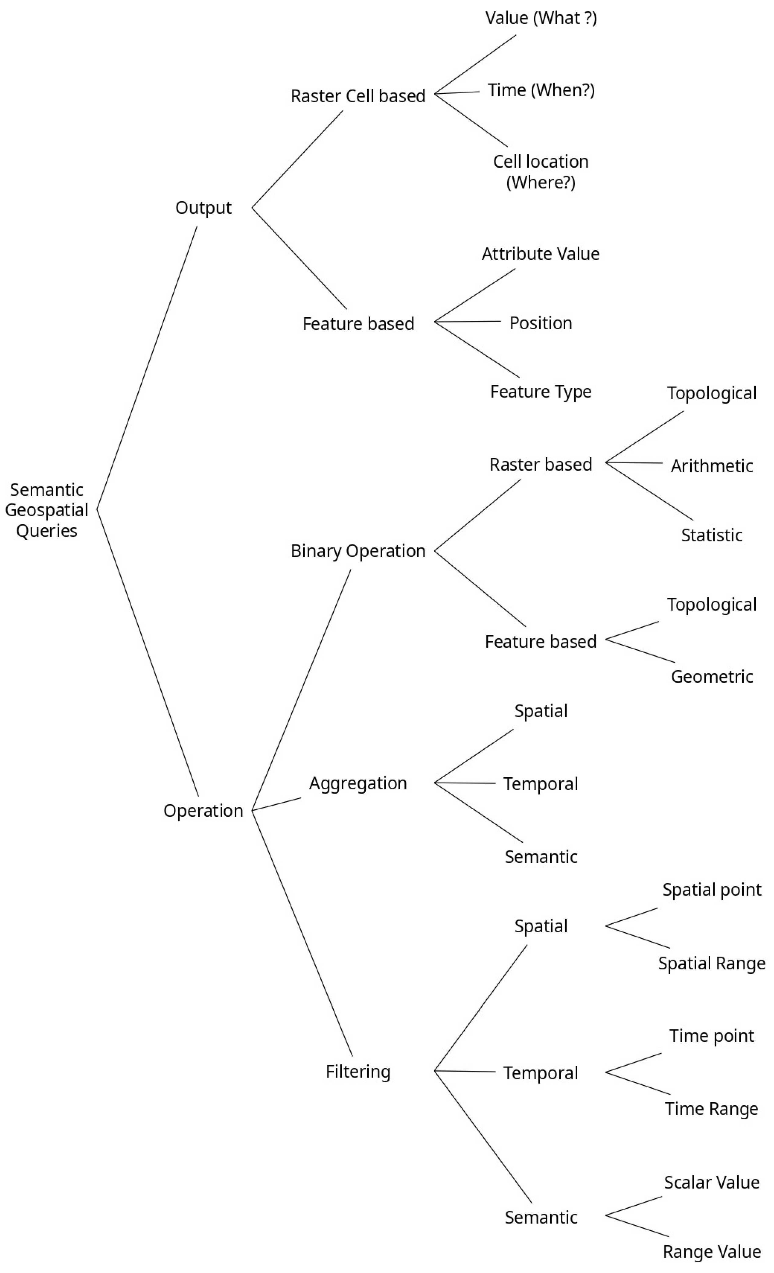
In this taxonomy, and at a high level of abstraction, we characterize any semantic geospatial query both by the nature of the operations that it involves and by the nature of the output that it might yield.

Regarding the nature of the operation, we distinguish three main ones: binary operation, aggregation, and filtering. The binary operation can be of raster type, which means that the two operands of such an operation are data cube/raster layers, or it could be feature-based, where the operands are features. These operations are principally topological, geometric, or arithmetic. For the aggregation operation, it could be spatial, which represents the operation of reducing variability within space; temporal, which, by analogy with space, is the operation of reducing variability over the time interval; or semantic, which represents the operation of reducing variability over the value range. The same goes for the filtering operation, which consists of the condition that the query must meet to give the final result. The filter used can also be spatial, temporal, or semantic (see Figure 5).

Note that there is no exclusivity between each type of operation. This implies that a geospatial query can, for example, include both aggregation and filtering operations. Similarly, aggregation can be spatial or temporal in the same query.

In terms of the output of a semantic geospatial query, it consists of the nature of the answer sought by the query, which could be raster-based, where the target could be the value, time, or location of the raster cell, or it could be feature-based, where the target is the value of an attribute or the position or the type of the feature (see Figure 5).

3.3.2. Scenarios and Classifications

We propose a set of geospatial queries that combine the information retrieval from the data cube with a set of features that are in the same spatial domain as the data cube (see

Table 2. List of the semantic geospatial queries that should be tested as scenarios for the use case.

	Query Code	Textual Description
Basic	Q1	What are the raster cells and their values related to the variable V between two times, $t_i$ and $t_j$?
	Q2	What are the raster cells and their values related to the variable V where these values are greater than the value $v_i$ between two times, $t_i$ and $t_j$?
	Q3	What are the raster cells and their values related to the variable V at the point $p_i$ between two times, $t_i$ and $t_j$?
	Q4	What are the raster cells and their values related to the variable V inside the region R between two times, $t_i$ and $t_j$?
Advenced	Q5	How is the spatial distribution of the maximum of the variable V within a feature f between two times, $t_i$ and $t_j$?
	Q6	How is the spatial distribution of the highest difference between two variables, $V_j$ and $V_k$, in each raster cell within a feature f during a period between $t_i$ and $t_j$?
	Q7	What and where is the maximum value of the variable V inside the feature $f_a$ of the type $T_a$ holding the maximum number of features of the type $T_b$ between two times, $t_i$ and $t_j$?
	Q8	How does the maximum value of the variable V evolve during the period between $t_i$ and $t_j$?
	Q9	When and where does the highest value of the variable V occur during the period between $t_i$ and $t_j$, and which features and their types does this value fall within?

). These queries represent a set of generic scenarios related to the study of any given geographic phenomenon. These queries are only a sample of the total number of scenarios we could obtain by using all the possibilities within our proposed geospatial query framework.

The first four queries are classified as basic since they are exclusively related to retrieving different patterns of information from data cubes over time without including any information about geospatial features. For instance, $Q1$ could be labeled a time range query (TRQ) since it is searching for the raster cells (i.e., spatial atoms) and their values over a time range. $Q2$ could be mostly termed as a field range query (FRQ) since it seeks to retrieve raster cells and their values that fall within a range of values related to a given distributed variable. $Q3$ might be considered mostly a spatial point query (SPQ) since it seeks to retrieve the raster cells and values related to a given spatial point. The last basic query, $Q4$, could be characterized as a spatial range query (SRQ) since it is concerned with retrieving the raster cells and their values that lie within a given spatial region. We give more accurate classifications regarding these four queries in both

Table 3. Classification of the set of spatiotemporal queries Queries based on the data cube and feature nature of output as well as their basic operations.

	Data Cube-Based Output		Data Cube Binary Operations		Feature-Based Outputs			Feature-Based Operations
Queries Ref	Value	Location/Cell	Topological	Arithmetic/Statistics	Attribute Value	Position	Type	Geometric (e.g., Buffer, Area)	Topologic
Q1	×	×
Q2	×	×							×
Q3	×	×							×
Q4	×	×
Q5	×	×							×
Q6	×	×		×
Q7	×	×				×			×
Q8	×	×							×
Q9	×	×			×	×	×		×

and

Table 4. Classification of the set of spatiotemporal queries based on the nature of aggregation and used filter.

	Aggregation-Based			Filter-Based
Queries Ref.	Spatial	Temporal	Semantic	Spatial		Temporal		Semantic
				0-Dimension	2-Dimension	Time Point	Time Range	Scalar	Range
Q1							×
Q2				×			×
Q3					×		×
Q4							×		×
Q5		×			×		×
Q6		×			×		×
Q7	×	×	×		×		×
Q8	×				×		×
Q9	×				×		×

.

On the other side, we consider the last five queries advanced ones. This is mainly because all these queries combine information related to geospatial features with the semantic data cube. These queries also apply to the processes of spatial and temporal aggregation. We characterize these queries as follows:

• Queries Q5 and $Q6$, for instance, first apply temporal aggregation over a time interval. However, $Q5$ applies it to a distributed variable, while $Q6$ performs a difference operation between two given distributed variables, which could be considered a map algebra operation qualified as a local one.
• $Q7$ applies spatial and temporal aggregation to find the maximum value of a given distributed variable. This value must be within the feature $f_i$ that contains the maximum number of features of the specific type $T_b$. Thus, this query additionally involves two spatial topological operations, one between the features of two entity types and the second between the selected feature and the data cube.
• $Q8$ applies only a spatial aggregation for each moment in a time interval over a given distributed variable V. This leads to a trajectory with a sequence of time-stamped value-point pairs.
• The last query, $Q9$, also applies spatial aggregation for each time point but also looks at which feature the trajectory of the highest value crosses and determines the type of these features. In addition, this query involves a spatial topology operation between the feature and the data cube.

The precise positioning of these advanced queries can be seen in Table 3 and Table 4. Additionally, each query mentioned in this table has a corresponding equivalent that effectively illustrates it through a specific example. The chosen illustration revolves around forest fire data, whereas raster data includes variables such as surface temperature and evapotranspiration. Similarly, features are represented using entities such as urban regions, territorial zones, and airports (see Section 5.1). Readers can refer to Appendix A, which covers queries $Q1$ to $Q4$. Similarly, for queries $Q5$ to $Q9$, they can refer to Section 5.2.

4. The Implementation of the Proposed Framework

In this section, we explain the overall architecture that our framework uses to implement the underlying concepts developed. In addition, we describe the VKG specifications that depict the process through which the framework was implemented.

4.1. System Architecture

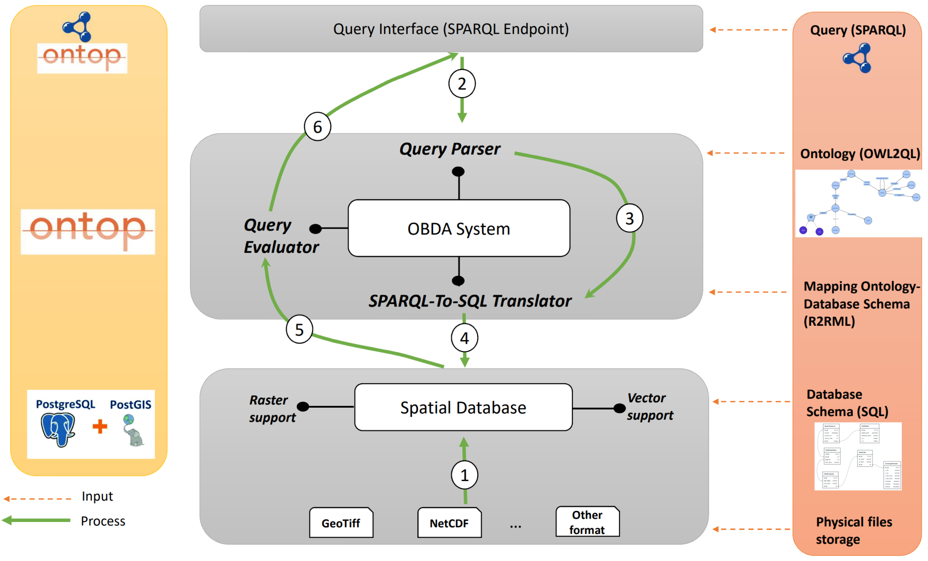
As shown in Figure 6, our system architecture is composed of three main layers:

• Data integration layer. This layer lies at the bottom of the architecture and involves integrating raw data from different geospatial sources, especially raster (e.g., Geotiff and NetCdf formats) and vector (e.g., Shapefiles and GML formats) data, within a spatial database that supports both raster and vector data (e.g., PostgreSQL/PostGIS, Oracle, etc.) using well-designed database schemas. In our case, after creating our database schemas in PostgreSQL, we extracted and loaded the data from their raw formats (ex. Netcdf, GeoTiff, etc.) along with their metadata into the selected PostgreSQL relational database. Then, we used PostGIS raster functions, mainly ST_PixelAsPoint, to extract the center of each pixel related to the coverage of the data cube and ST_Value to extract the value of such pixel. The aim of this process (i.e., process 1) was to fill the schema of our database and, in particular, the three tables of FieldAtom, SpaceTimeLoc, and FieldPropValue (see Figure 7).
• Ontology-based data access (OBDA) layer. This layer represents the core of the system. At this layer, a semantic model in the form of an ontology is defined in order to provide a formal and high-level representation of the domain of interest. In addition, the mapping must be defined to link the classes and properties of the ontology to the tables and attributes of the database schemas. There are three main components in this layer that are responsible for four related processes:

  -

  Query parser: this component is the upper part of the SPARQL query engine. Its main role is to receive SPARQL queries and perform a syntax check to verify their correctness and compliance with the query language syntax. Once queries have passed the syntax check, this component forwards them to the translation module for further processing (process 3).

  -

  SPARQL-to-SQL translator: this component receives the analyzed SPARQL query as input and uses the VKG specification, which includes the ontology and its mapping. With the support of a reasoner that uses the axioms defined in the ontology, it transforms the query into an SQL equivalent. The reformulated query is then sent for execution to the spatial database engine (process 4).

  -

  Query Evaluator: this component utilizes the output of an SQL query executed within the spatial database engine (process 5). It assesses the query result and converts it into a collection of RDF triples, without physically materializing the data. The resulting set of RDF triples includes the original RDF triples representing the queried records from the database as well as newly inferred RDF triples. The entire collection of RDF triples generated for a specific query is known as the virtual knowledge graph (VKG). Finally, the result of this translation is sent to the query interface for visualization (process 6).

• Query interface for SPARQL layer. This layer consists of a front-end interface that allows the interaction between users and the proposed system. Users can query the classes and relations of the ontology using the SPARQL query language (process 2) and then display the results of their queries.

4.2. The VKG Specifications

As explained earlier, to implement our framework, we need to define the VKG specification triple $(O,M,S)$ with three key ingredients: the ontology, O, which is defined in Section 3.2.3, the data source schema, S, which structures the data source into a database schema, and the mapping, M, which connects the classes and properties of the ontology to the tables and attributes of the database schema.

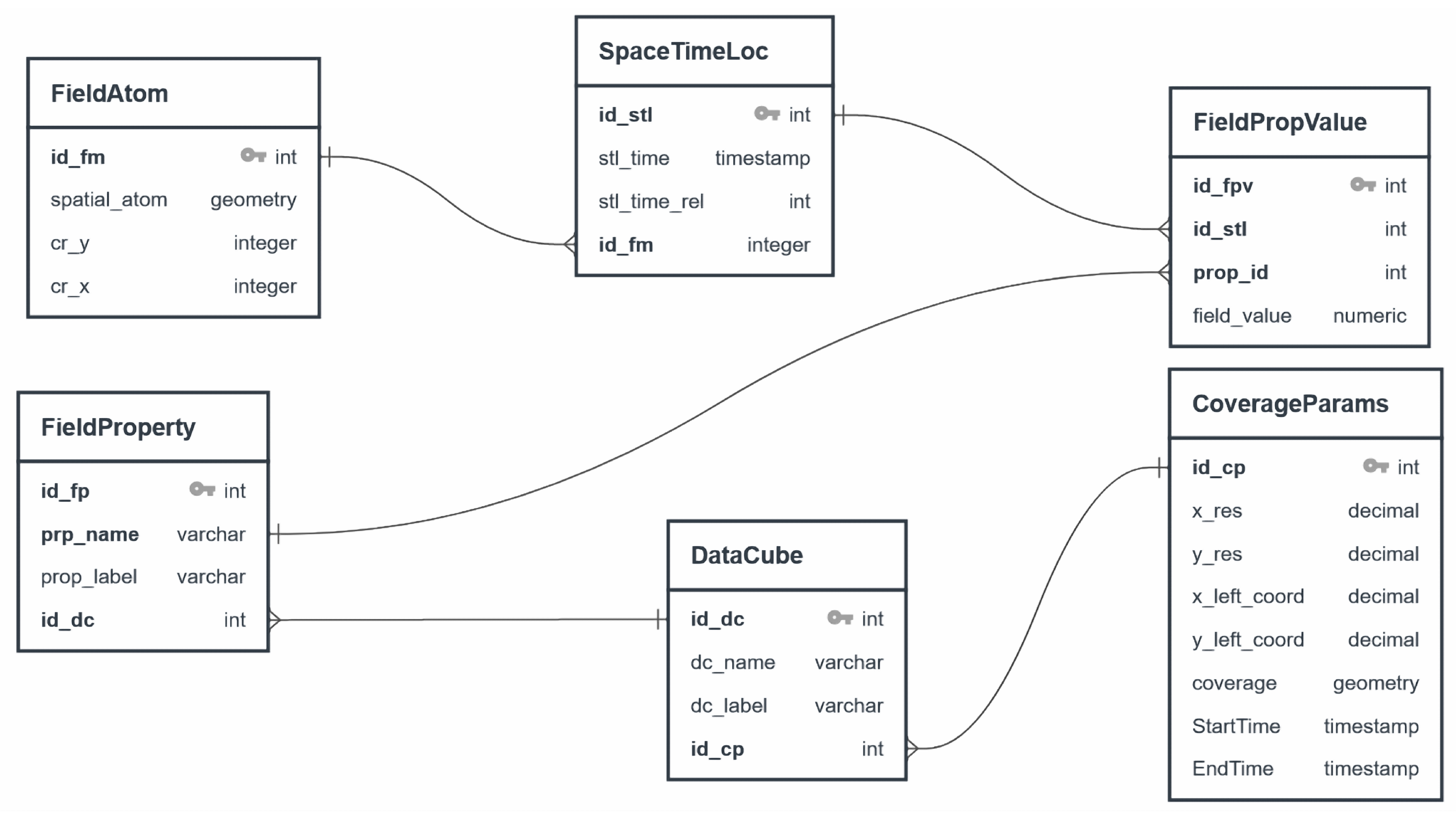
For the design of the data source schema, we define the database design model that is most suitable for our defined ontology. This data model is designed with respect to the normal form to benefit from all optimizations deployed in the VKG system as well as to avoid some redundancies and self-joining during query execution and evaluation. The logical data model (see Figure 7) is composed of six interrelated tables that correspond to the classes defined in our ontology.

For instance, the class dcb:SpaceTimeLoc is represented by the table SpaceTimeLoc, where each instance is characterized by a temporal component (i.e., stl_time attribute) and by a spatial component that is an instance of the spatial domain of a data cube. This spatial domain is modeled as a table named FieldAtom, which stores the geometries of all cells in a given data cube. Any given spatiotemporal location should have one and only one spatial component (i.e., a raster cell), and this spatial component could spawn or be the source of multiple spatiotemporal locations depending on the size of the temporal dimension. Thus, to represent such a functional relationship, we move the primary key of the table FieldAtom to the table SpaceTimeLoc and consider it a foreign key.

The data cube class is mainly defined on the basis of the relationship between a spatiotemporal location and a subset of property-value pairs. This subset is materialized by the table FieldPropValue. This table mainly contains a foreign key (prop_id attribute), which refers to the table FieldProperty containing the set of all distributed variable names (i.e., the field properties). Correspondingly, the table FieldPropValue contains the value (field_value attribute), which is associated with a specific property and characterizes a unique spatiotemporal location.

Finally, since a data cube can be mainly characterized by the set of its properties (i.e., variables) along with the set of parameters related to its spatial and temporal coverage, we therefore create a table named DataCube and we link it to the table FieldProperty, where each property of this table characterizes one and only one instance of the DataCube table. In a similar way, we create the table CoverageParams, which contains all the parameters that characterize the spatial and temporal extent of a given data cube. A data cube must be characterized by only one instance of the table CoverageParams.

In order to link the database schema S to the ontology O, we need to define a mapping M between them. Following the definition in [31,45], a mapping, M, consists of a set of assertions of the form:

$$\begin{array}{c}\hfill m:\varphi (a_1,a_2,a_3,\dots ,a_n)\hookrightarrow \psi (a_1,a_2,a_3,\dots ,a_n)\end{array}$$

• In this case, $\varphi (a_1,a_2,a_3,\dots ,a_n)$ represents a query on a data source schema, S, that selects the attributes $(a_1,a_2,a_3,\dots ,a_n)$ of all tables generated by such a query. In the case where the data source schema S is relational, such a query is expressed using SQL.
• $\psi (a_1,a_2,a_3,\dots ,a_n)$ represents a RDF triplet statement specifying the way to use RDF terms constructed from database values to instantiate classes and properties. More precisely, such a model indicates either that an RDF term (representing an object) is an instance of a class, or that such a term is related by a property to another term representing an object or a literal value.

The standard language for representing the mapping, M, is defined by the W3C R2RML specification. For instance, in 

Table 5. Mapping between the database schema and the ontology.

Mapping Assertions
Mapping ID	Source: SQL Query	Target: Turtle Template
FieldAtom	select id_fm, st_astext(field_loc) as field_loc, coord_rel_x, coord_rel_y from FieldAtom	dcb:fad-{id_fm} a dcb:FieldAtom;     dcb:xRelCoord {coord_rel_x}⌃⌃xsd:integer;     dcb:yRelCoord {coord_rel_y}⌃⌃xsd:integer;     dcb:asFieldWKT {field_loc}⌃⌃geo:wktLiteral.
SpaceTimeLocation	select from SpaceTimeLoc	dcb:stl-{id_stl} a dcb:SpaceTimeLoc;   dcb:hasRelTime {time_index}⌃xsd:integer;   dcb:hasDateTime {stl_time}⌃⌃dateTimeStamp;   dcb:hasSpatialRef dcb:fad-{id_fm}.
Field_prop_value	select from FieldPropValue	dcb:fpval-{id_stlfv} a dcb:FieldPropValue;   dcb:hasFieldValue {fvalue};   dcb:hasVariableName {prop_name};   dcb:hasFieldProp dcb:fpv-{prop_id};   dcb:hasSTL dcb:stl-{id_stl}.
DataCube_coverage	select id_ps, ps_name, ps_label, dc.id_cp, upperleftx, upperlefty, dc_width, dc_hight from property_set dc, coverage_params cp where dc.id_cp = cp.id_cp	dcb:dc-{id_ps} a dcb:DataCube;   dcb:dcHasName {ps_name}⌃xsd:string;   dcb:dcHasLabel {ps_label}⌃⌃xsd:string;   dcb:hasCoverageParams dcb:cp-{id_cp}. dcb:cp-{id_cp} a dcb:CoverageParams;   dcb:xLeftCorner {upperleftx}⌃⌃xsd:double;    dcb:yLeftCorner {upperlefty}⌃⌃xsd:double;   dcb:xspatialSize {dc_width}⌃⌃xsd:integer;   dcb:yspatialSize {dc_hight}⌃⌃xsd:integer
Field_Property	select from FieldProperty	dcb:fpv-{id_prop} a dcb:FieldPropVar;   dcb:hasPropName {prop_name}⌃⌃xsd:string;   dcb:hasPropSet dcb:dc-{ps_id}.

, we define a set of mapping assertions to associate our database schema, S, with our ontology terms. For example, in the mapping assertion called spaceTimeLocation, the source SQL query $\varphi$ outputs the attributes (id_stl, time_index, stl_time, id_fm), which are mapped to the RDF triple statement $\psi$. The statement $\psi$ binds the identifier of the table spaceTimeLoc (i.e., id_stl attribute) with the URI of the class dcb:SpaceTimeLocation in order to uniquely identify each instance of this class. Then, in the same mapping, we associate the attribute stl_time with the data property dcb:hasDateTime and the foreign key id_fm with the data property dcb:hasSpatialRef, which refer respectively to the temporal and spatial components of each instance of the class dcb:SpaceTimeLocation.

Once our relational schemas are populated, we obtain the source database, D, which will serve as the population source of our ontology through the mapping, M. This population consists of a set of RDF assertions. Conceptually speaking, we call $M\left(D\right)$ the set of RDF assertions on a database, D, through the mapping, M. Then, by applying the semantics and axioms related to our ontology, we could derive a new RDF graph, such as the relational data on the source, which is denoted $G_M{}_{,}{}_D$.

In practice, the ontology is populated only at the time of the SPARQL query execution. The SPARQL query is rewritten into a SQL query based on the mapping, M, and the result is transformed into a knowledge graph, as illustrated in Section 4.1.

5. Use Cases and System Performances Evaluation

We apply our approach to a specific use case using a given dataset by formulating and executing nine scenarios in the form of spatiotemporal queries. We distinguish between basic queries that focus on retrieving information only from raster layers and advanced queries that combine raster layers with discrete features.

5.1. Use Case and Dataset

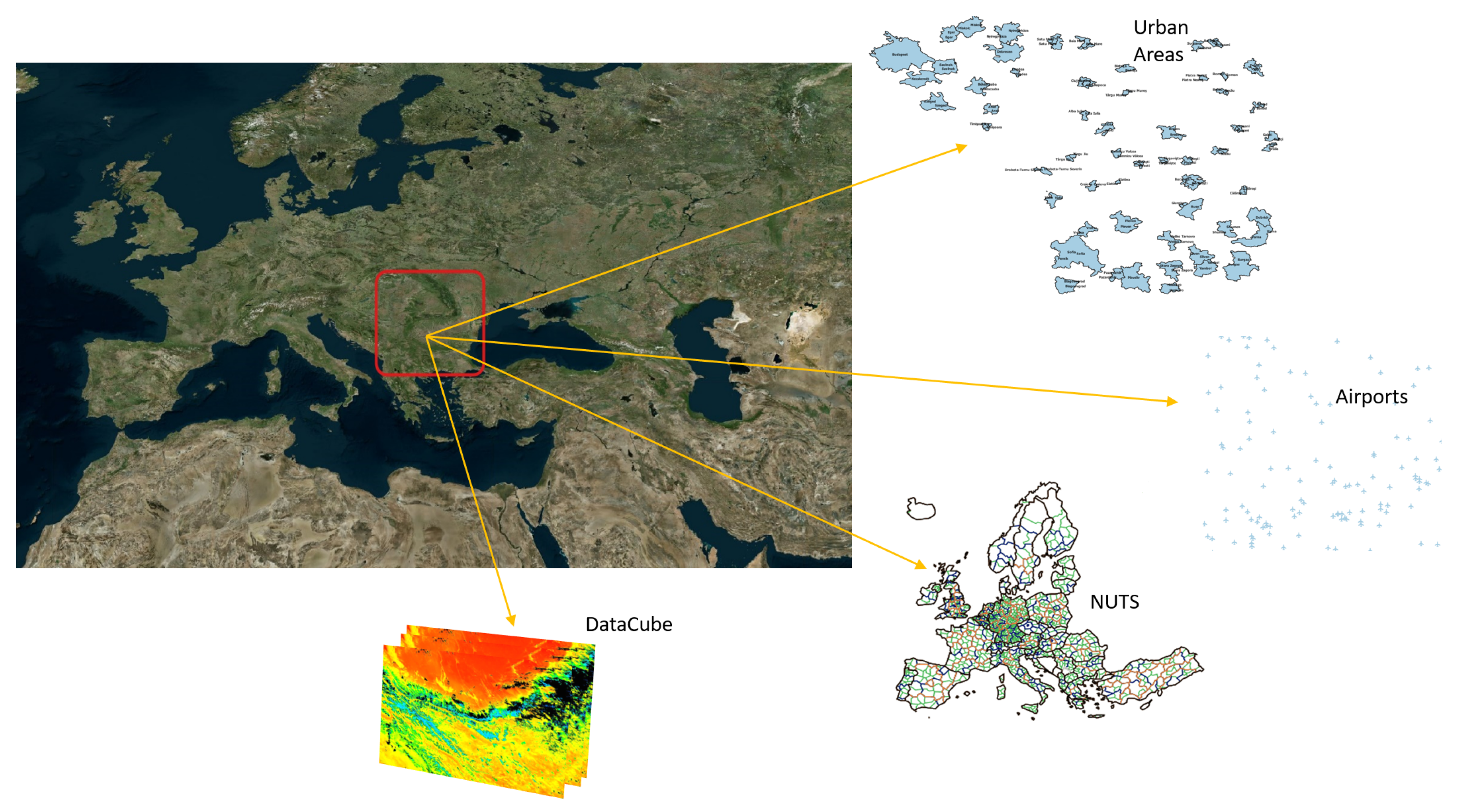
The modeling approach was tested and applied to the forest fire data, as future climate variability is expected to increase the risk and severity of forest fires in many regions, especially in southern Europe and the Mediterranean region (see Figure 8). Properly managing and exploring raster data cube variables, such as land surface temperature, in their spatial context can help scientists better recognize areas or regions most likely to experience forest fires in the future.

For this experiment, we use two main types of geospatial datasets (see Figure 8). The first type is feature-based data that consists of three vector layers, namely urban areas, airports, and NUTS [46]. NUTS (nomenclature of territorial units for statistics) is a hierarchical system dividing the economic territory of the EU and the UK into three levels known as NUTS 1 (major socio-economic regions), NUTS 2 (basic regions for the application of regional policies), and NUTS 3 (small regions for specific diagnoses).

The second dataset type is data cubes, consisting of sequences of time-stamped raster layers of multiple variables. In our case, we select four variables that are resampled at a daily temporal resolution and with a spatial resolution of 1 km. These variables are land surface temperature during the day, land surface temperature at the night, leaf area index, and evapotranspiration. The spatial size of each temporal raster layer is 117 × 142 pixels, whereas the temporal dimension we pick up starts from 15 March 2009 and ends on 3 May 2009, and consists of 50 temporal snapshots for each variable (daily temporal resolution).

5.2. SPARQL Query Formulation and Visualization

In this section, we express the set of queries that are presented in Table 2. We map these queries to our dataset to make them more specific and utilize SPARQL to formulate and answer such queries. We use the query editor extension developed by the Ontop system for the Protégé software [33]. We only display the SPARQL formulations relative to the advanced queries (i.e., from Q5 to Q9). However, the reader can find the SPARQL formulations relative to the first four queries in Appendix A. To reformulate queries, we need to define a list of prefixes that must be declared for each query being reformulated (see

Table 6. List of prefixes used for SPARQL queries.

Acronym	URL
geo	<http://www.opengis.net/ont/geosparql/> (accessed on 10 June 2023)
geof	http://www.opengis.net/def/function/geosparql (accessed on 10 June 2023)
units	http://www.opengis.net/def/uom/OGC/1.0/ (accessed on 10 June 2023)
crs	http://www.opengis.net/def/crs/OGC/1.3/CRS84/ (accessed on 10 June 2023)
geo-sf	http://www.opengis.net/def/dataType/OGC-SF/1.0/ (accessed on 10 June 2023)
dcb	http://www.semanticweb.org/OntologyRasterDataCube/ (accessed on 10 June 2023)
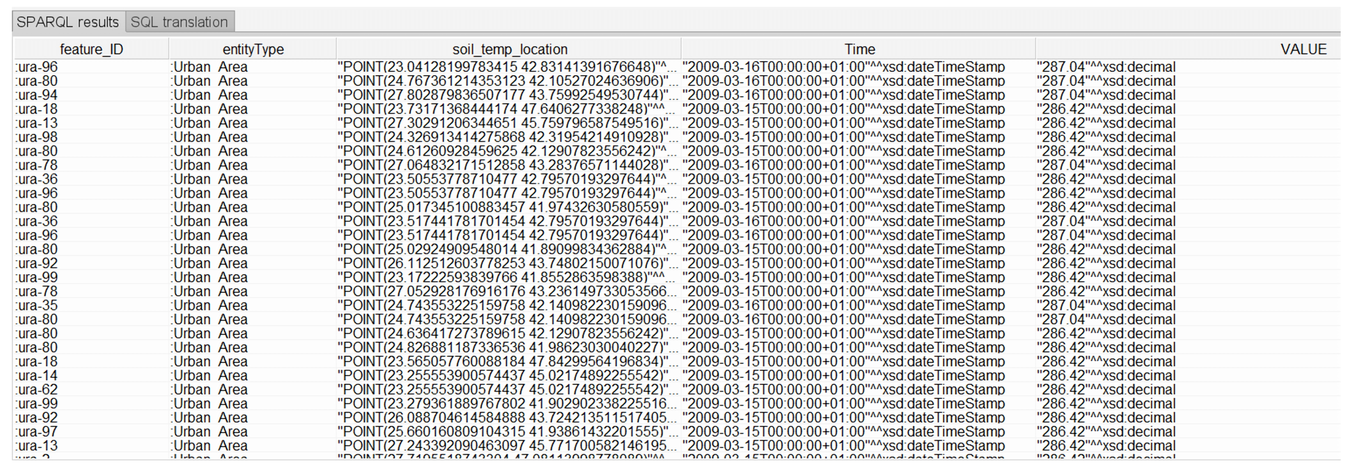
geop	http://www.opengis.net/def/property/OGC-GeoSPARQL/1.0/ (accessed on 10 June 2023)

). For query execution, the Ontop system is employed. This system provides outcomes in either tabular or JSON format and concurrently generates a translation of the SPARQL query into an SQL query optimized for PostGIS. Utilizing the existing connection interface between QGIS and PostGIS, these SQL queries are then executed within the QGIS platform, facilitating the subsequent visualization of results within the QGIS environment.

• Q5  What is the spatial distribution of the maximum soil temperature within the urban area named Sofia between two times, 15 March 2009 and 25 March 2009?

• Q6  What is the spatial distribution of the highest difference in soil temperature in each raster cell between day and night within a feature f during a time interval between 15 March 2009 and 25 March 2009?

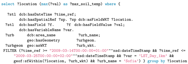
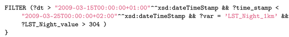
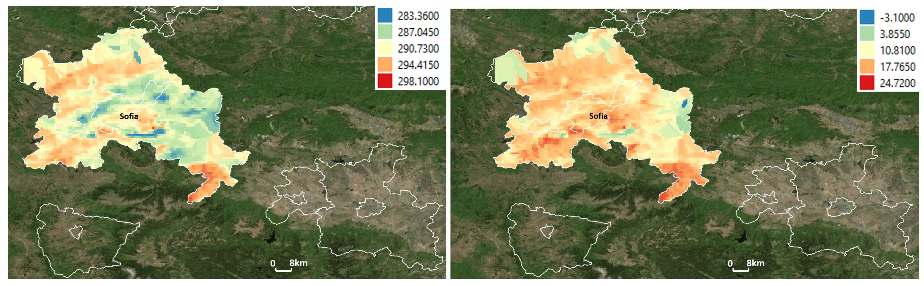
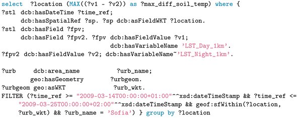
Q5 applies temporal aggregation along with a spatial filter to extract the maximum value of soil temperature for each raster cell in the selected urban area. Figure 9 (left) shows the visualization of the query result from Q5, with colors from blue to red indicating the maximum soil temperature from low to high. While Q6 applies the same operations, it calculates, in addition, the difference between day and night soil temperatures, which requires crossing two data cubes. In Figure 9 (right), the red-colored area shows a strong disparity, while the blue-colored area shows a relative concordance between day and night soil temperatures.

• Q7 What is the maximum soil temperature inside the entity holding the maximum number of airports between two times, 15 March 2009 and 14 May 2009?

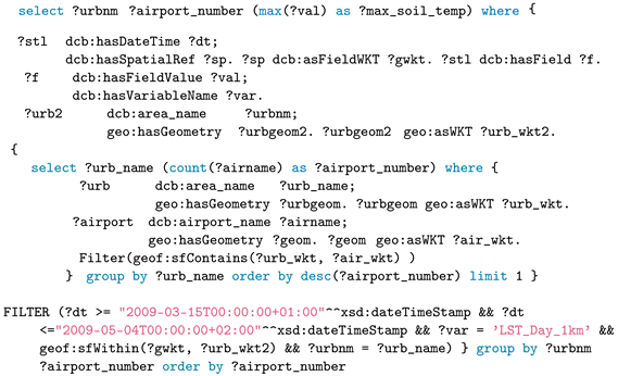
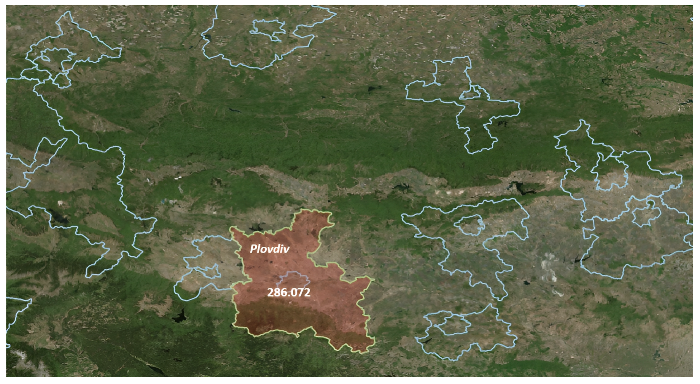
Q7 uses a subquery to make a selection of the urban area containing the maximum number of airports and then returns that area for applying spatial and temporal aggregation to select the maximum soil temperature value. The resulting map shows the selected area along with the maximum value, which is 286.072 (see Figure 10).

• Q8  How does the maximum soil temperature evolve during the period between 15 March 2009 and 25 March 2009?

• Q9  When and where did the highest soil temperature value occur during the period between 15 March 2009 and 17 March 2009 and what are the entities and their types that this value falls within?

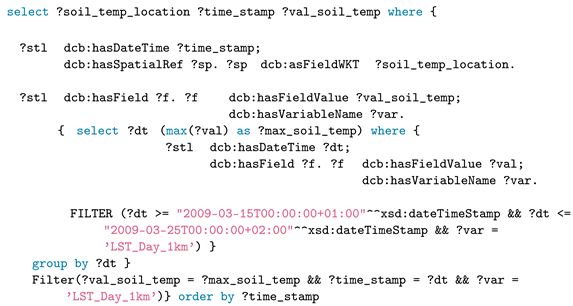
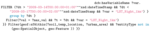
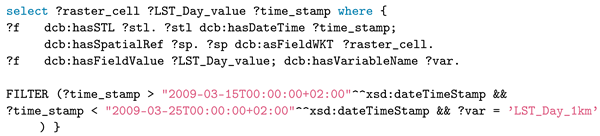
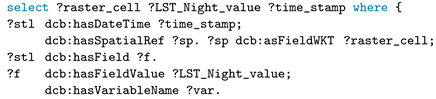
Q8 uses a subquery to calculate the maximum value for each time. This sequence of values is then returned and used in the outer query to find the locations corresponding to each maximum value. Figure 11 shows the path that was drawn to track the maximum at each time.

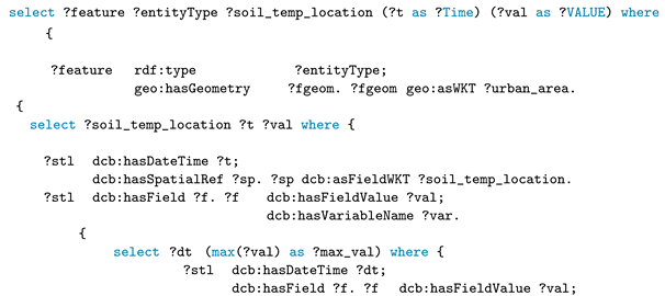
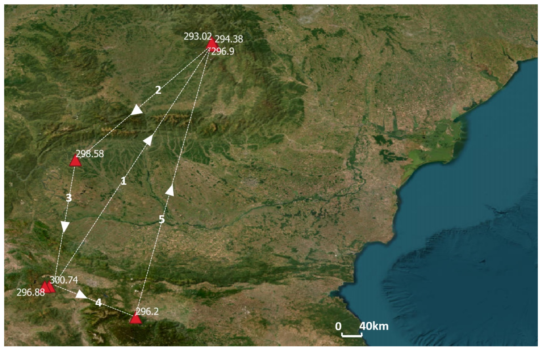
Q9 involves two nested subqueries. The first selects the maximum value of the soil temperature for each time and returns this sequence to the outer subquery to find all locations corresponding to each maximum value in this sequence. We then use a spatial filter with a topological relationship to try to find the geometric features in which these locations are contained. Finally, using the reasoning capabilities of the system, the query can infer the entity type of each geometric feature that meets the spatial criteria. Figure 12 shows the result of this query.

5.3. Performance Evaluation

This section evaluates the computational performance of our implemented framework. This experimentation consists of two parts:

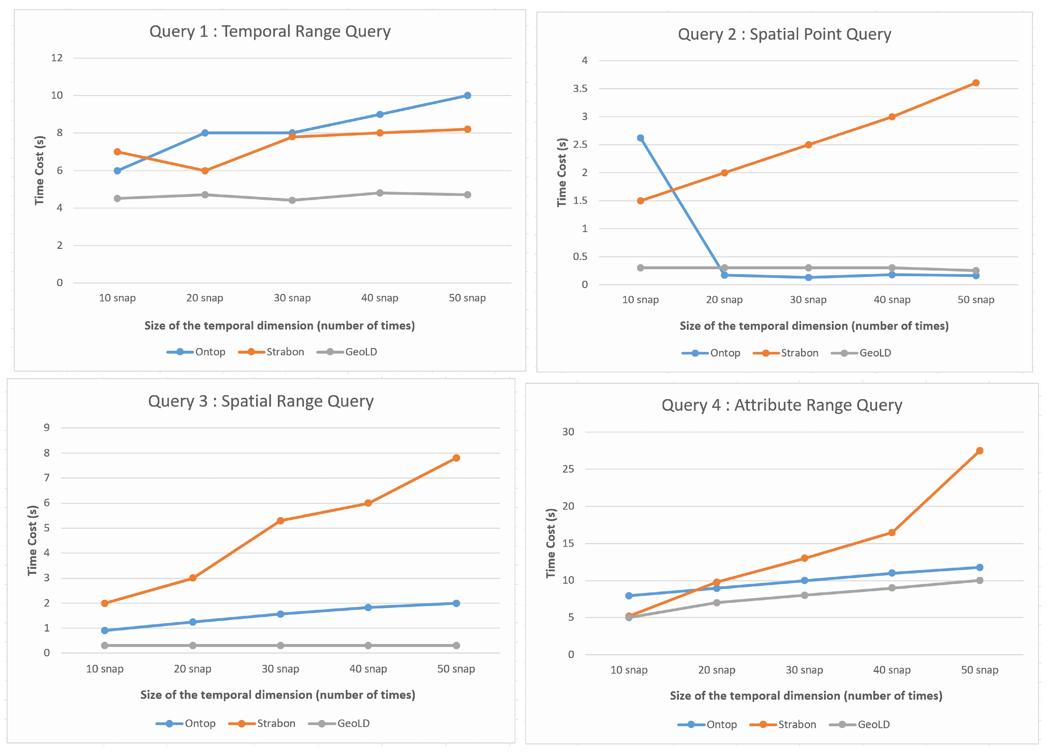
• In the first experiment, we compare our framework implemented on the basis of the Ontop system against GeoLD and Strabon. For this comparison, we use the four basic spatiotemporal queries formulated in Appendix A. We examine the runtime performance of each query and observe how the graphical curves evolve as the size of the temporal dimension (i.e., the number of time-stamped layers) increases for each system. These experiments have been conducted and are illustrated in Figure 13.
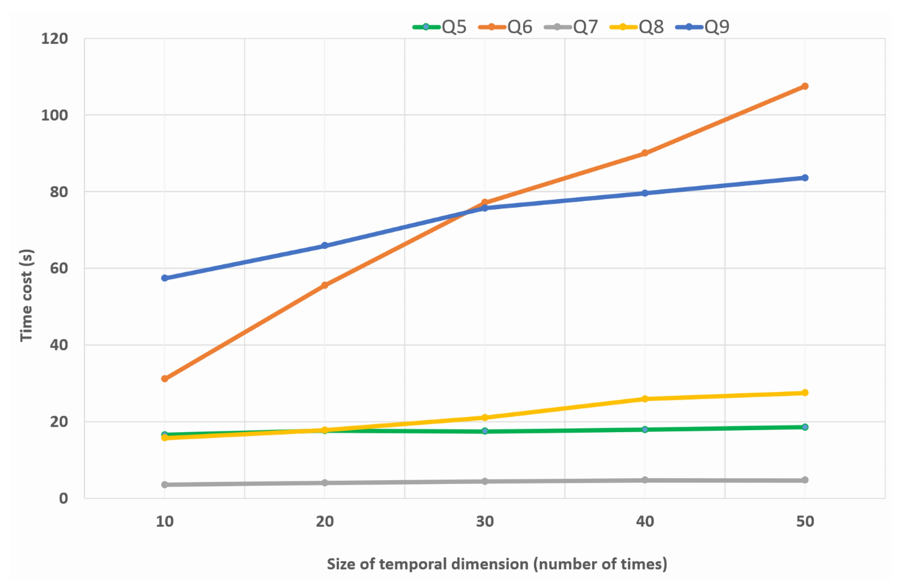
• The second experiment consists of examining, using the Ontop system, the evolution of the execution time of advanced geospatial queries reformulated in Section 5.2. Similarly, we examine the runtime cost as the size of the temporal dimension increases. However, in this evaluation, a comparison is made between and among these queries to see how the Ontop system behaves with each of them. This is illustrated in Figure 14.

For each query in the experiments, three separate consecutive calls are made to collect their average response times. For the first part of the experiment, we can clearly see from Figure 13 that for the three queries, Q2, Q3, and Q4, the framework implemented under the VKG system performs well, and scales quite well with the growing size of the temporal dimension. The performance of Ontop is very close to that of the GeoLD system, even though the GeoLD system uses an array-based database system (Rasdaman), which is considered the most efficient for storing and querying raster data cubes. Both Ontop and GeoLD significantly outperform the Strabon system for these queries. However, with respect to Q1, Ontop does not perform as well as GeoLD and Strabon. This may be due to several reasons. Indeed, the wider the temporal range of the query is, the less efficient the spatial index of the database can be. The reason is that all raster cells of the study area are requested, which leads to a high amount of requested spatiotemporal cells. Thus, the on-the-fly translation process of this output data into RDF format that is performed by the Ontop system becomes costly and has a significant impact on the performance and scalability of the system. In this case, a time range query with a spatial filter could be highly desirable to obtain a better response. In addition, a partitioning strategy for temporal data in PostgreSQL could help improve the scalability of the system. Finally, improving the computational performance of the algorithm that translates geospatial data on the fly into RDF format could help reduce the cost of the query answer.

In the second part of the experiment, we can observe three main patterns: the first one shows that Ontop performs very well for three queries, Q5, Q7, and Q8. These queries involve a time range with a spatial filter (Q5), a spatial and temporal aggregation (Q7), and a spatial-only aggregation (Q8). The second trend is related to the behavior of Ontop regarding the Q9 query, which involves spatial aggregation together with a spatial filter. In addition, it involves a reasoning operation to infer the entity types from selected instances. The execution time in this case becomes more expensive but the system still shows acceptable scalability. The last trend is related to query Q6. It is obvious that when the size of input data increases, the system shows poor scalability and the curve tends to have exponential growth. This is due to the fact that this query involves a binary operation between two data cubes. This type of query can be performed naturally and efficiently when the data cubes are encoded as multidimensional arrays. However, with a VKG system like Ontop and its relational databases, this type of query requires the development of optimal operators or functions that can efficiently handle such binary operations.

It is worth mentioning that, to perform such an experiment, we used the Ontop version 4.2.1, which is integrated with the Protégé software. This package enables the user to load the ontology, define the mapping, and reformulate SPARQL queries. The generic data model schema has been implemented in the PostgreSQL 13 software. Tests were performed on a Dell LAT 7520 with 3 GHz Max, 11th generation, Intel Core i7, and 32 GB of RAM. The operating system used was Windows 10.

6. Conclusions and Discussion

This paper proposed a framework to enable the semantic integration and advanced querying of raster data cubes based on VKG. In this framework, we defined a semantic representation model for raster data cubes as a module that extends the GeoSPARQL ontology. With such a model, we could combine the semantics of raster data cubes with feature-based models that involve geometries as well as spatial/topological relationships. This allowed us to formulate spatiotemporal queries using SPARQL in a natural way by using ontological concepts at an appropriate level of abstraction. In order to evaluate the expressivity of any semantic representation model, we confronted it with a set of scenarios that, in our case, were a set of geospatial queries. We further presented a taxonomy within which each query can find its semantic positioning. We then took a sample of scenarios and classified them according to this taxonomy. Furthermore, we explained the system architecture that enabled us to implement our proposed framework. We applied our approach to forest fire data and formulated nine basic and advanced spatiotemporal queries to retrieve information from only raster and from both raster and vector layers, respectively. To evaluate the computational performance of our implemented framework, we designed an experiment with two parts: In the first one, we compared our framework implemented using the Ontop system against GeoLD and Strabon. In the second one, we examined the runtime cost as the size of the temporal dimension increased, and made a comparison between and among these queries to see how the system behaved with each query.

In conclusion, the proposed framework expands the ability to express enhanced geospatial queries and enables the intelligent integration of a semantic data cube. Furthermore, the implementation of this framework shows reasonable performance, especially with respect to the complexity of the formulated queries. However, for some queries, the system shows weak performance and scalability. This mainly concerns queries involving binary operations on data cubes (e.g., arithmetic, topological, etc.). In addition, other operations are not yet properly supported. This includes rolling or focal operations, as well as operations that manipulate the shape and dimensions of the data cube. For future work, this part still needs to be developed and supported efficiently at the SPARQL level in order to enable the full manipulation and integration of the data cube. Another challenge for future work is to develop an approach that not only handles static geometric features but also evolving entities and to combine them with raster data cubes, which can help develop a powerful and intelligent analytical query system for dynamic GIS.