

A Multi-Framework of Google Earth Engine and GEV for Spatial Analysis of Extremes in Non-Stationary Condition in Southeast Queensland, Australia


 ,
, 
 and
and 
Abstract
:1. Introduction
2. Materials and Methods
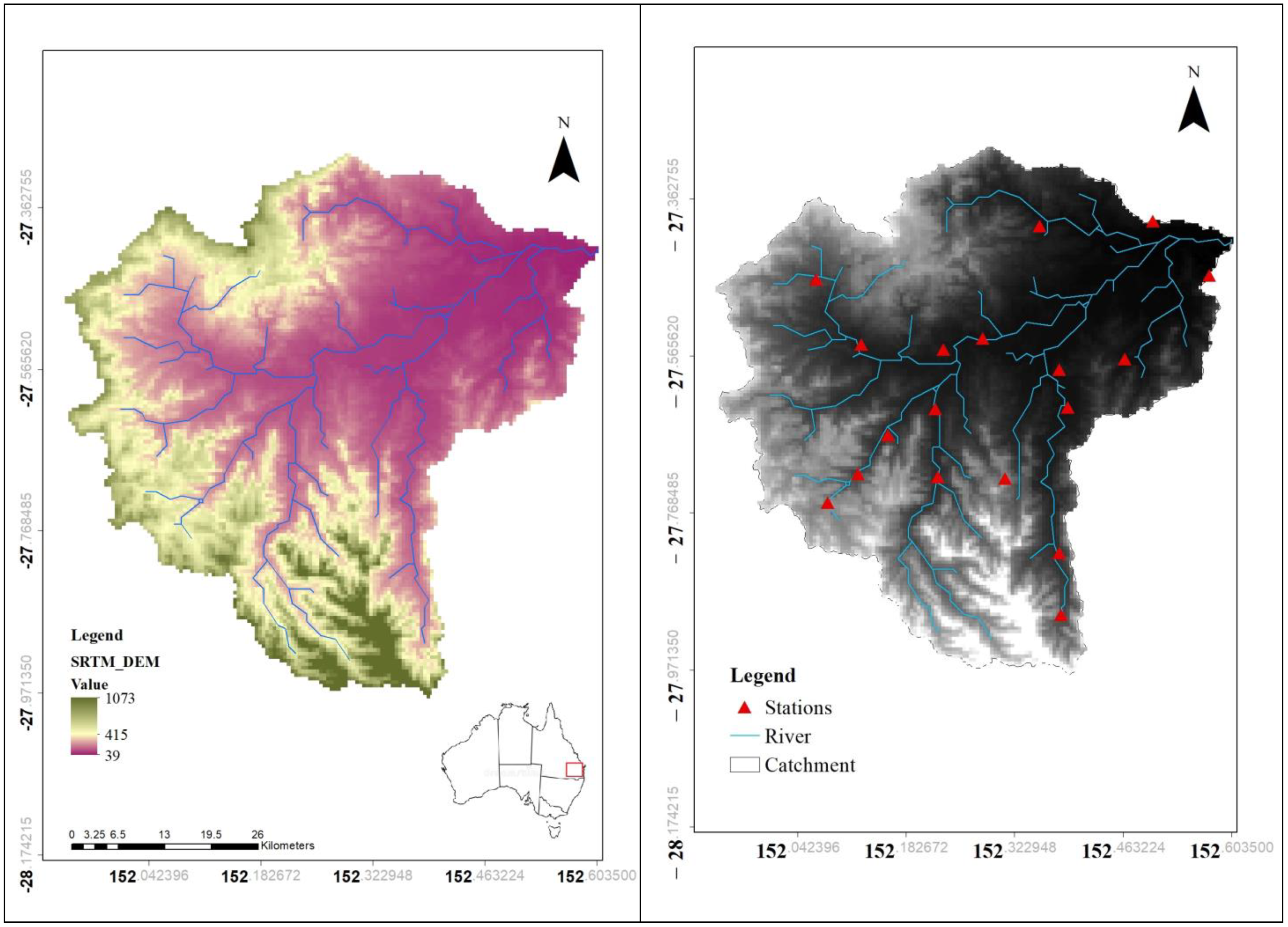
2.1. Study Region
2.2. Observed and Global Climate Dataset
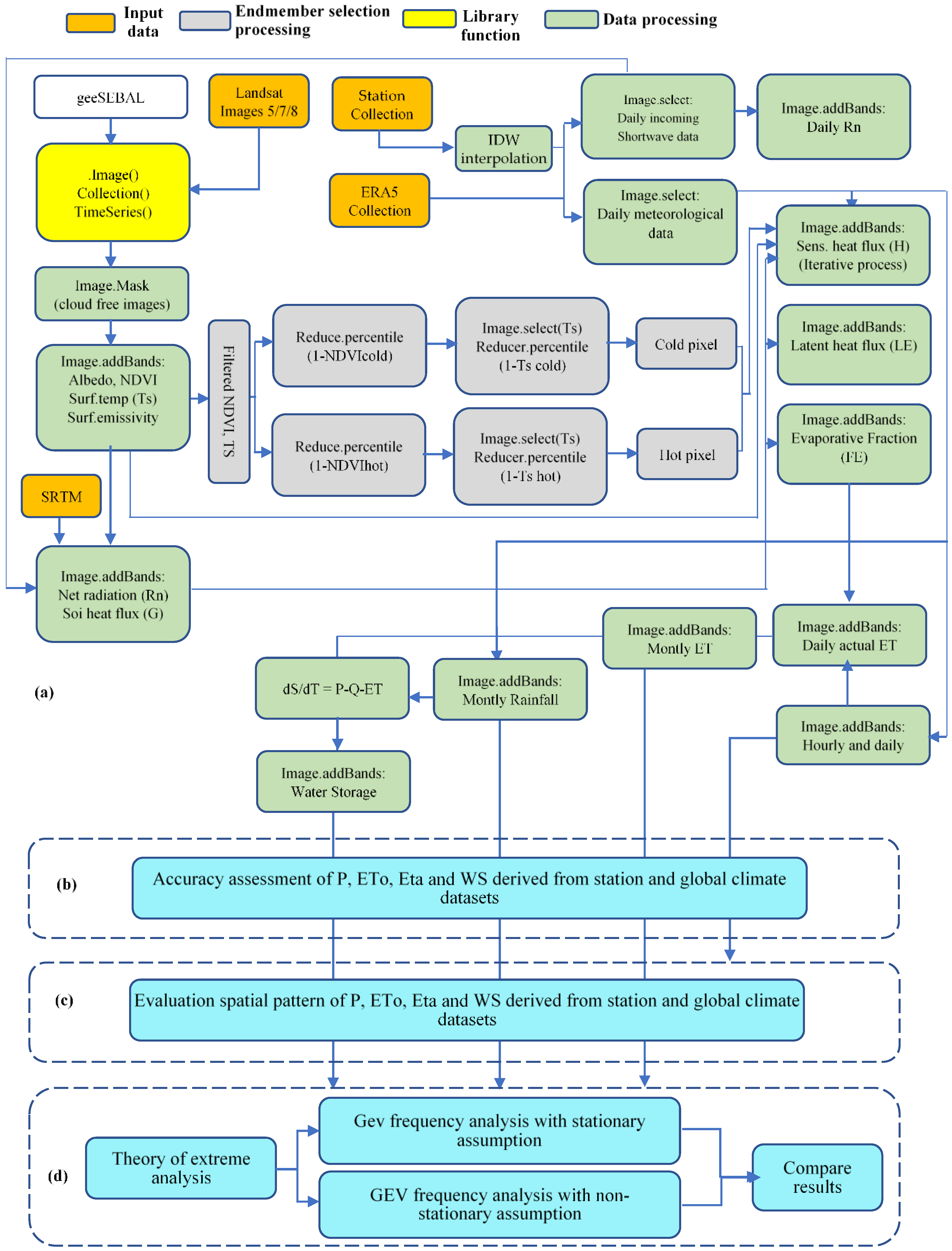
2.3. Google Earth Engine Application: The geeSEBAL Algorithm
2.4. Assessing Extremes in a Non-Stationary Approach Using GEV Model
3. Results
3.1. Station Data and ERA5 Land Reanalysis Feeding into geeSEBAL as Meteorological Inputs
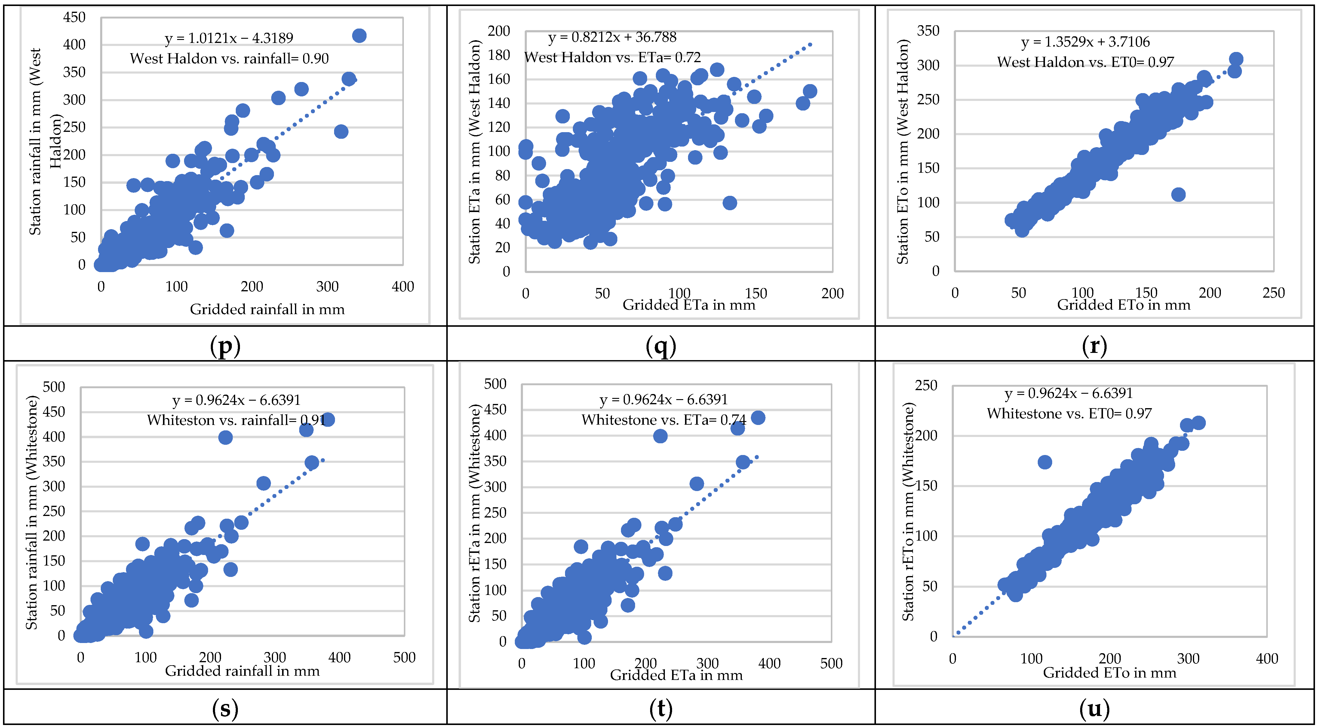
3.2. Validation of geeSEBAL ETa and ETo and Rain across Stations
3.3. Results of Trends
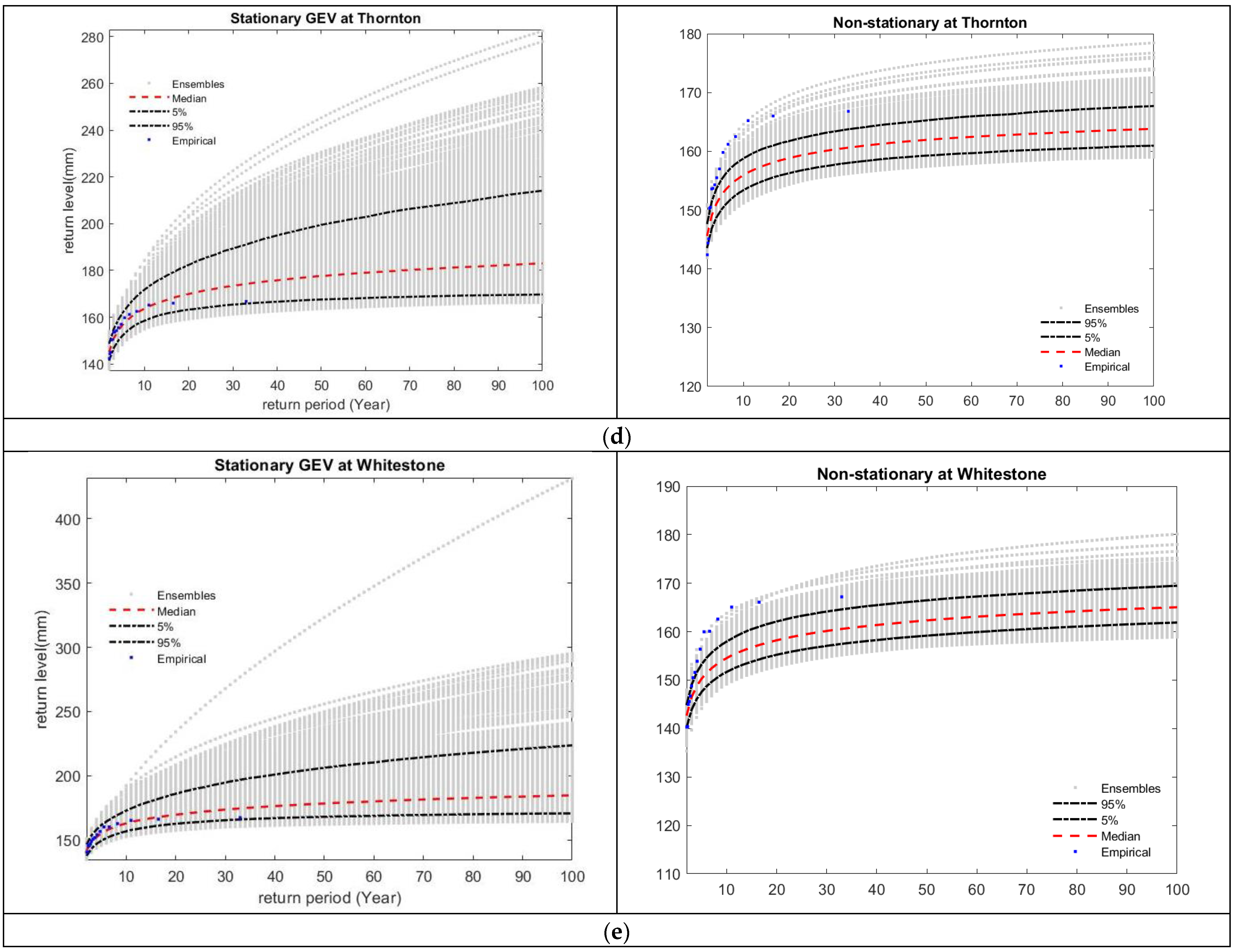
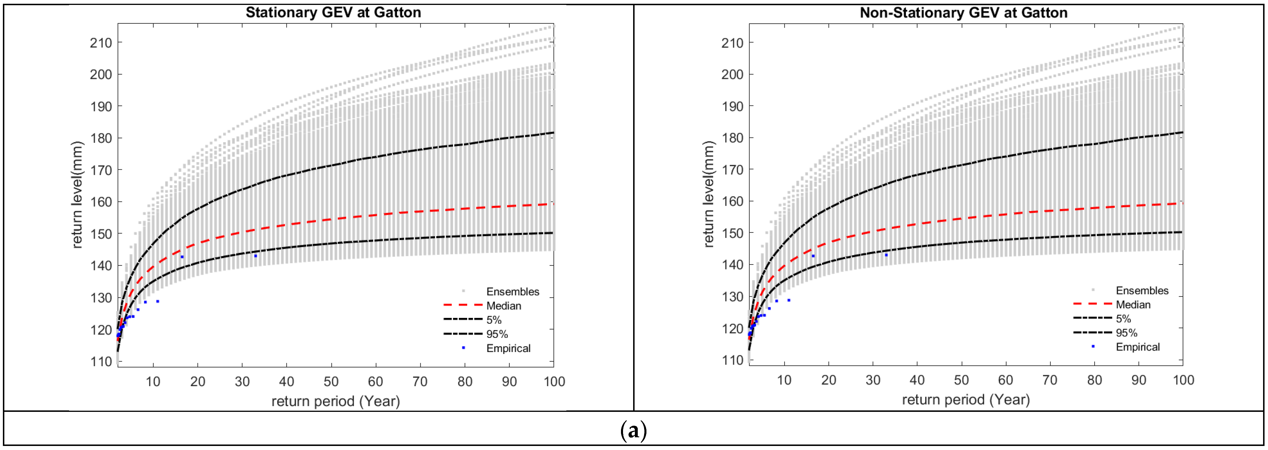
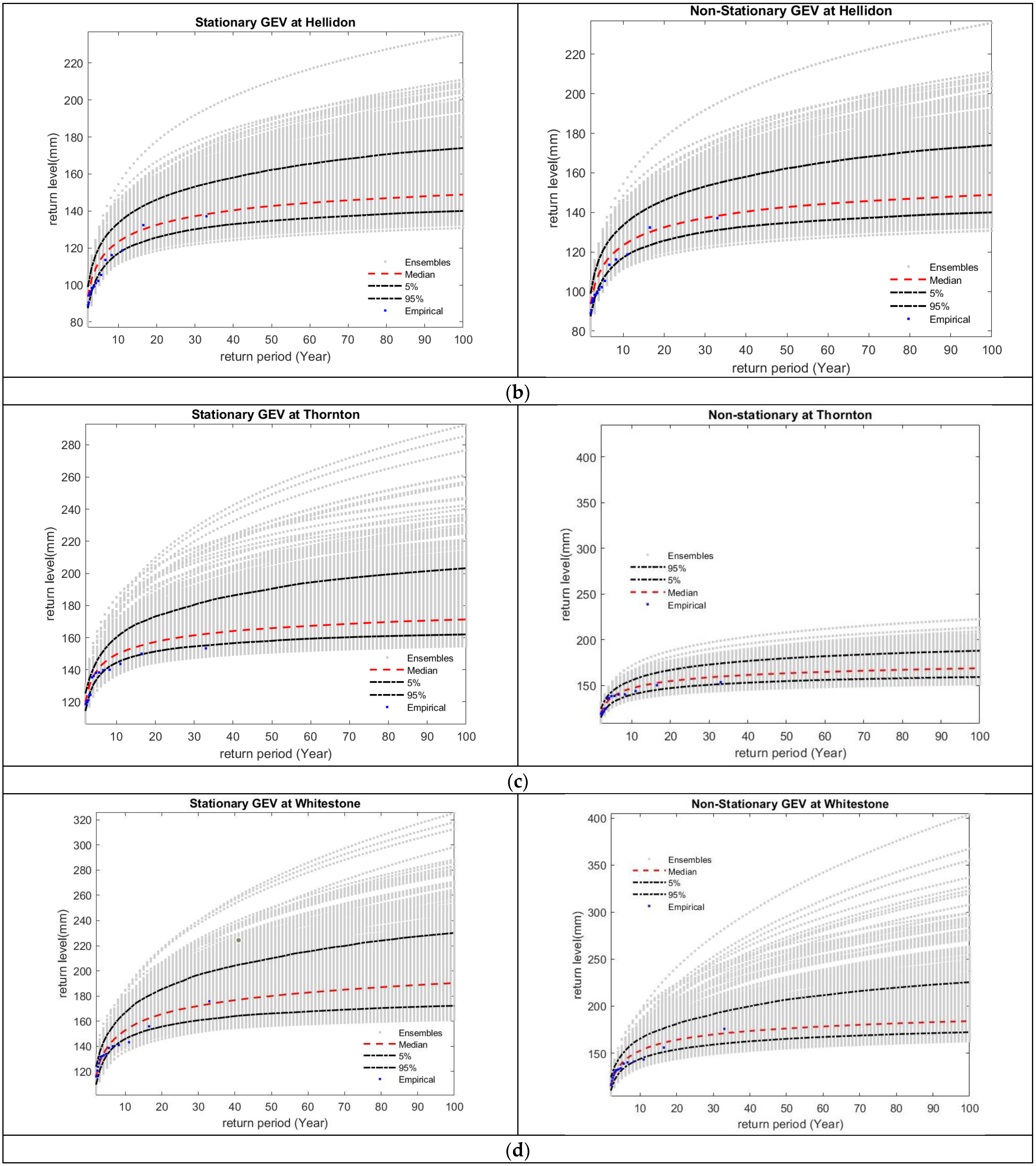
3.4. Results of Stationary and Non-Stationary Analysis for Rainfall
3.5. Results of Stationary and Non-Stationary Analysis for Evapotranspiration
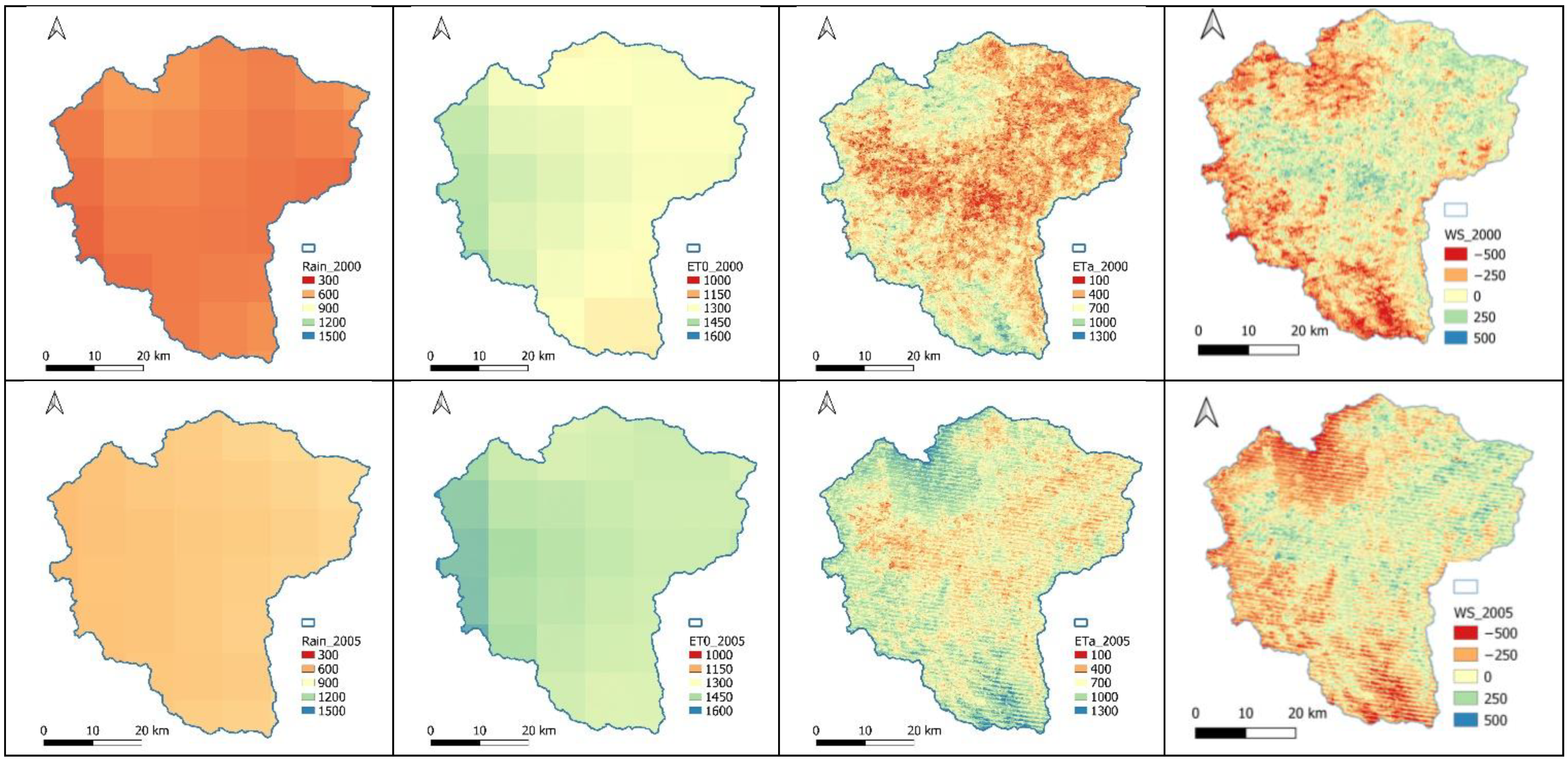
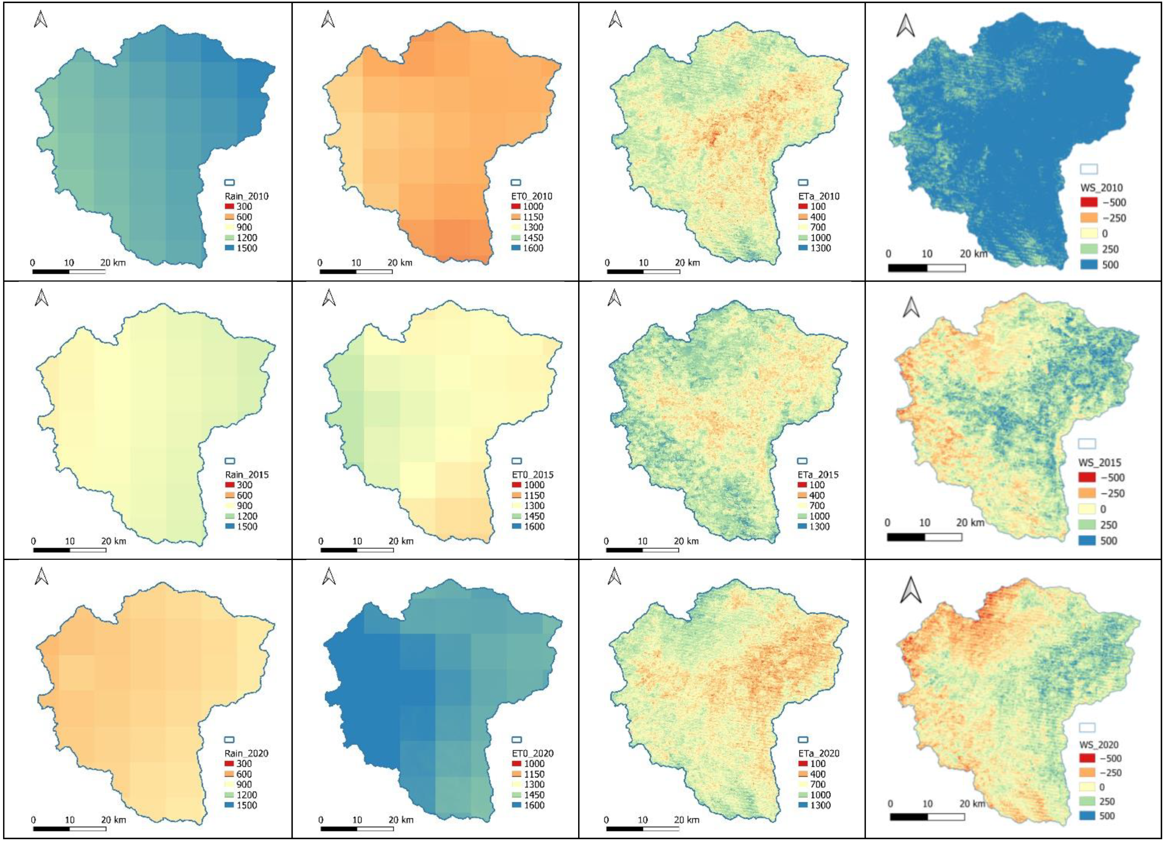
3.6. Results of Stationary and Non-Stationary Analysis for Water Storage
4. Discussion
5. Conclusions
Author Contributions
Funding
Data Availability Statement
Acknowledgments
Conflicts of Interest
References
- Cheng, L.; AghaKouchak, A.; Gilleland, E.; Katz, R.W. Non-stationary extreme value analysis in a changing climate. Clim. Chang. 2014, 127, 353–369. [Google Scholar] [CrossRef]
- IPCC. Climate Change 2007: Synthesis Report. Contribution of Working Groups I, II and III to the Fourth Assessment Report of the Intergovernmental Panel on Climate Change; Core Writing Team, Pachauri, R.K., Reisinger, A., Eds.; Cambridge University Press: Cambridge, UK, 2007; p. 104. [Google Scholar]
- Salas, J.; Obeysekera, J.; Vogel, R. Techniques for assessing water infrastructure for nonstationary extreme events: A review. Hydrol. Sci. J. 2018, 63, 325–352. [Google Scholar] [CrossRef]
- Cooley, D. Extreme value analysis and the study of climate change. Clim. Chang. 2009, 97, 77–83. [Google Scholar] [CrossRef]
- Love, C.A.; Skahill, B.E.; Russell, B.T.; Baggett, J.S.; AghaKouchak, A. An Effective Trend Surface Fitting Framework for Spatial Analysis of Extreme Events. Geophys. Res. Lett. 2022, 49, e2022GL098132. [Google Scholar] [CrossRef]
- Salas, J.D.; Obeysekera, J. Revisiting the concepts of return period and risk for nonstationary hydrologic extreme events. J. Hydrol. Eng. 2014, 19, 554–568. [Google Scholar] [CrossRef]
- Cooley, D. Return periods and return levels under climate change. In Extremes in a Changing Climate; AghaKouchak, A., Easterling, D., Hsu, K., Schubert, S., Sorooshian, S., Eds.; Water Science and Technology Library; Springer: Berlin/Heidelberg, Germany, 2013; Volume 65, pp. 97–114. [Google Scholar]
- Abbs, D.; McInnes, K.; Rafter, T. The impact of climate change on extreme rainfall and coastal sea levels over south-east Queensland. Div. Mar. Atmos. Res. Commonw. Sci. Ind. Res. Organ. Aust. 2007. Available online: https://www.cmar.csiro.au/e-print/open/2007/abbsdj_c.pdf (accessed on 2 September 2023).
- Mpelasoka, F.; Hennessy, K.; Jones, R.; Bates, B. Comparison of suitable drought indices for climate change impacts assessment over Australia towards resource management. Int. J. Climatol. A J. R. Meteorol. Soc. 2008, 28, 1283–1292. [Google Scholar] [CrossRef]
- Zhang, H.; Wang, B.; Li Liu, D.; Zhang, M.; Feng, P.; Cheng, L.; Yu, Q.; Eamus, D. Impacts of future climate change on water resource availability of eastern Australia: A case study of the Manning River basin. J. Hydrol. 2019, 573, 49–59. [Google Scholar] [CrossRef]
- Laipelt, L.; Kayser, R.H.B.; Fleischmann, A.S.; Ruhoff, A.; Bastiaanssen, W.; Erickson, T.A.; Melton, F. Long-term monitoring of evapotranspiration using the SEBAL algorithm and Google Earth Engine cloud computing. ISPRS J. Photogramm. Remote Sens. 2021, 178, 81–96. [Google Scholar] [CrossRef]
- Kiem, A.S.; Johnson, F.; Westra, S.; van Dijk, A.; Evans, J.P.; O’Donnell, A.; Rouillard, A.; Barr, C.; Tyler, J.; Thyer, M. Natural hazards in Australia: Droughts. Clim. Chang. 2016, 139, 37–54. [Google Scholar] [CrossRef]
- Van Loon, A.F.; Stahl, K.; Di Baldassarre, G.; Clark, J.; Rangecroft, S.; Wanders, N.; Gleeson, T.; Van Dijk, A.I.; Tallaksen, L.M.; Hannaford, J. Drought in a human-modified world: Reframing drought definitions, understanding, and analysis approaches. Hydrol. Earth Syst. Sci. 2016, 20, 3631–3650. [Google Scholar] [CrossRef]
- Ajami, H.; Sharma, A.; Band, L.E.; Evans, J.P.; Tuteja, N.K.; Amirthanathan, G.E.; Bari, M.A. On the non-stationarity of hydrological response in anthropogenically unaffected catchments: An Australian perspective. Hydrol. Earth Syst. Sci. 2017, 21, 281–294. [Google Scholar] [CrossRef]
- Petheram, C.; Potter, N.; Vaze, J.; Chiew, F.; Zhang, L. Towards better understanding of changes in rainfall-runoff relationships during the recent drought in south-eastern Australia. In Proceedings of the 19th International Congress on Modelling and Simulation, Perth, Australia, 12–16 December 2011; pp. 12–16. [Google Scholar]
- IPCC. Climate Change 2014: Synthesis Report. Contribution of Working Groups I, II and III to the Fifth Assessment Report of the Intergovernmental Panel on Climate Change; IPCC: Geneva, Switzerland, 2014. [Google Scholar]
- Bastiaanssen, W.G.; Menenti, M.; Feddes, R.A.; Holtslag, A.A.M. A remote sensing surface energy balance algorithm for land (SEBAL). 1. Formulation. J. Hydrol. 1998, 212, 198–212. [Google Scholar] [CrossRef]
- Liou, Y.-A.; Kar, S.K. Evapotranspiration estimation with remote sensing and various surface energy balance algorithms—A review. Energies 2014, 7, 2821–2849. [Google Scholar] [CrossRef]
- Gebremichael, M.; Wang, J.; Sammis, T.W. Dependence of remote sensing evapotranspiration algorithm on spatial resolution. Atmos. Res. 2010, 96, 489–495. [Google Scholar] [CrossRef]
- Allen, R.G.; Tasumi, M.; Morse, A.; Trezza, R.; Wright, J.L.; Bastiaanssen, W.; Kramber, W.; Lorite, I.; Robison, C.W. Satellite-based energy balance for mapping evapotranspiration with internalized calibration (METRIC)—Applications. J. Irrig. Drain. Eng. 2007, 133, 395–406. [Google Scholar] [CrossRef]
- Bezerra, B.G.; da Silva, B.B.; dos Santos, C.A.; Bezerra, J.R. Actual evapotranspiration estimation using remote sensing: Comparison of SEBAL and SSEB approaches. Adv. Remote Sens. 2015, 4, 234. [Google Scholar] [CrossRef]
- Allen, R.G.; Burnett, B.; Kramber, W.; Huntington, J.; Kjaersgaard, J.; Kilic, A.; Kelly, C.; Trezza, R. Automated calibration of the METRIC-Landsat evapotranspiration process. JAWRA J. Am. Water Resour. Assoc. 2013, 49, 563–576. [Google Scholar] [CrossRef]
- Cheng, L.; AghaKouchak, A. Nonstationary precipitation intensity-duration-frequency curves for infrastructure design in a changing climate. Sci. Rep. 2014, 4, 7093. [Google Scholar] [CrossRef]
- Jones, B.; Tebaldi, C.; O’Neill, B.C.; Oleson, K.; Gao, J. Avoiding population exposure to heat-related extremes: Demographic change vs climate change. Clim. Chang. 2018, 146, 423–437. [Google Scholar] [CrossRef]
- Khaliq, M.N.; St-Hilaire, A.; Ouarda, T.B.; Bobée, B. Frequency analysis and temporal pattern of occurrences of southern Quebec heatwaves. Int. J. Climatol. A J. R. Meteorol. Soc. 2005, 25, 485–504. [Google Scholar] [CrossRef]
- Rainham, D.G.; Smoyer-Tomic, K.E. The role of air pollution in the relationship between a heat stress index and human mortality in Toronto. Environ. Res. 2003, 93, 9–19. [Google Scholar] [CrossRef]
- Huth, R.; Kyselý, J.; Pokorná, L. A GCM simulation of heat waves, dry spells, and their relationships to circulation. Clim. Chang. 2000, 46, 29–60. [Google Scholar] [CrossRef]
- Ouarda, T.B.; Charron, C. Nonstationary temperature-duration-frequency curves. Sci. Rep. 2018, 8, 15493. [Google Scholar] [CrossRef] [PubMed]
- Mazdiyasni, O.; Sadegh, M.; Chiang, F.; AghaKouchak, A. Heat wave intensity duration frequency curve: A multivariate approach for hazard and attribution analysis. Sci. Rep. 2019, 9, 11609. [Google Scholar] [CrossRef] [PubMed]
- Ball, J.; Babister, M.; Nathan, R.; Weinmann, P.; Weeks, W.; Retallick, M.; Testoni, I. Australian Rainfall and Runoff-A Guide to Flood Estimation; Commonwealth of Australia: Canberra, Australia, 2019. [Google Scholar]
- Pakdel Khasmakhi, H.; Vazifedoust, M.; Paudyal, D.R.; Chadalavada, S.; Alam, M.J. Google Earth Engine as Multi-Sensor Open-Source Tool for Monitoring Stream Flow in the Transboundary River Basin: Doosti River Dam. ISPRS Int. J. Geo-Inf. 2022, 11, 535. [Google Scholar] [CrossRef]
- Sarker, A.; Ross, H.; Shrestha, K.K. A common-pool resource approach for water quality management: An Australian case study. Ecol. Econ. 2008, 68, 461–471. [Google Scholar] [CrossRef]
- WetlandInfo. Wetland Management Resources in Queensland. Available online: https://wetlandinfo.des.qld.gov.au/wetlands/ (accessed on 6 March 2022).
- Kiem, A.S.; Vance, T.R.; Tozer, C.R.; Roberts, J.L.; Dalla Pozza, R.; Vitkovsky, J.; Smolders, K.; Curran, M.A. Learning from the past. Using palaeoclimate data to better understand and manage drought in South East Queensland (SEQ), Australia. J. Hydrol. Reg. Stud. 2020, 29, 100686. [Google Scholar] [CrossRef]
- Vance, T.; Roberts, J.; Plummer, C.; Kiem, A.; Van Ommen, T. Interdecadal Pacific variability and eastern Australian megadroughts over the last millennium. Geophys. Res. Lett. 2015, 42, 129–137. [Google Scholar] [CrossRef]
- Lockyer Creek wiki 2022. Available online: https://en.wikipedia.org/wiki/Lockyer_Creek (accessed on 14 May 2022).
- Cui, T.; Raiber, M.; Pagendam, D.; Gilfedder, M.; Rassam, D. Response of groundwater level and surface-water/groundwater interaction to climate variability: Clarence-Moreton Basin, Australia. Hydrogeol. J. 2018, 26, 593–614. [Google Scholar] [CrossRef]
- Armstrong, M.S.; Kiem, A.S.; Vance, T.R. Comparing instrumental, palaeoclimate, and projected rainfall data: Implications for water resources management and hydrological modelling. J. Hydrol. Reg. Stud. 2020, 31, 100728. [Google Scholar] [CrossRef]
- CSIRO; BOM. Climate Change in Australia Information for Australia’s Natural Resource Management Regions: Technical Report; CSIRO and Bureau of Meteorology: Canberra, Australia, 2015. [Google Scholar]
- Jeffrey, S.J.; Carter, J.O.; Moodie, K.B.; Beswick, A.R. Using spatial interpolation to construct a comprehensive archive of Australian climate data. Environ. Model. Softw. 2001, 16, 309–330. [Google Scholar] [CrossRef]
- Ramezani, M.R.; Yu, B.; Tarakemehzadeh, N. Satellite-derived spatiotemporal data on imperviousness for improved hydrological modelling of urbanised catchments. J. Hydrol. 2022, 612, 128101. [Google Scholar] [CrossRef]
- Mission, N.S.R.T. Shuttle Radar Topography Mission (SRTM) Global. Distributed by OpenTopography. 2013. Available online: https://www.fdsn.org/networks/detail/GH/ (accessed on 15 September 2022).
- Gorelick, N.; Hancher, M.; Dixon, M.; Ilyushchenko, S.; Thau, D.; Moore, R. Google Earth Engine: Planetary-scale geospatial analysis for everyone. Remote Sens. Environ. 2017, 202, 18–27. [Google Scholar] [CrossRef]
- Kayser, R.H.; Ruhoff, A.; Laipelt, L.; de Mello Kich, E.; Roberti, D.R.; de Arruda Souza, V.; Rubert, G.C.D.; Collischonn, W.; Neale, C.M.U. Assessing geeSEBAL automated calibration and meteorological reanalysis uncertainties to estimate evapotranspiration in subtropical humid climates. Agric. For. Meteorol. 2022, 314, 108775. [Google Scholar] [CrossRef]
- Gonçalves, I.Z.; Ruhoff, A.; Laipelt, L.; Bispo, R.; Hernandez, F.B.T.; Neale, C.M.U.; Teixeira, A.H.d.C.; Marin, F.R. Remote sensing-based evapotranspiration modeling using geeSEBAL for sugarcane irrigation management in Brazil. Agric. Water Manag. 2022, 274, 107965. [Google Scholar] [CrossRef]
- Foga, S.; Scaramuzza, P.L.; Guo, S.; Zhu, Z.; Dilley Jr, R.D.; Beckmann, T.; Schmidt, G.L.; Dwyer, J.L.; Hughes, M.J.; Laue, B. Cloud detection algorithm comparison and validation for operational Landsat data products. Remote Sens. Environ. 2017, 194, 379–390. [Google Scholar] [CrossRef]
- Vazifedoust, M. Development of an Agricultural Drought Assessment System: Integration of Agrohydrological Modelling, Remote Sensing and Geographical Information; Wageningen University and Research: Wageningen, The Netherlands, 2007. [Google Scholar]
- Carey, B.; Stone, B.; Shilton, P.; Norman, P. Soil Conservation Guidelines for Queensland Chapter 4. In The Empirical Version of the Rational Method; Department of Environment and Resource; Queensland Government: Queensland, Australia, 2015. [Google Scholar]
- Madsen, H. Time Series Analysis; CRC Press: Boca Raton, FL, USA, 2007. [Google Scholar]
- Durocher, M.; Burn, D.H.; Ashkar, F. Comparison of estimation methods for a nonstationary Index-Flood Model in flood frequency analysis using peaks over threshold. Water Resour. Res. 2019, 55, 9398–9416. [Google Scholar] [CrossRef]
- Moisello, U. On the use of partial probability weighted moments in the analysis of hydrological extremes. Hydrol. Process. Int. J. 2007, 21, 1265–1279. [Google Scholar] [CrossRef]
- Coles, S.; Bawa, J.; Trenner, L.; Dorazio, P. An Introduction to Statistical Modeling of Extreme Values; Springer: Berlin/Heidelberg, Germany, 2001; Volume 208. [Google Scholar]
- Morrison, J.E.; Smith, J.A. Stochastic modeling of flood peaks using the generalised extreme value distribution. Water Resour. Res. 2002, 38, 41-1–41-12. [Google Scholar] [CrossRef]
- Mann, H.B. Nonparametric tests against trend. Econom. J. Econom. Soc. 1945, 13, 245–259. [Google Scholar] [CrossRef]
- Xu, C.-y.; Gong, L.; Jiang, T.; Chen, D.; Singh, V. Analysis of spatial distribution and temporal trend of reference evapotranspiration and pan evaporation in Changjiang (Yangtze River) catchment. J. Hydrol. 2006, 327, 81–93. [Google Scholar] [CrossRef]
- Da Silva, R.M.; Santos, C.A.; Moreira, M.; Corte-Real, J.; Silva, V.C.; Medeiros, I.C. Rainfall and river flow trends using Mann–Kendall and Sen’s slope estimator statistical tests in the Cobres River basin. Nat. Hazards 2015, 77, 1205–1221. [Google Scholar] [CrossRef]
- Nyikadzino, B.; Chitakira, M.; Muchuru, S. Rainfall and runoff trend analysis in the Limpopo river basin using the Mann Kendall statistic. Phys. Chem. Earth Parts A/B/C 2020, 117, 102870. [Google Scholar] [CrossRef]
- Burkey, J. A Non-Parametric Monotonic Trend Test Computing Mann-Kendall Tau, Tau-b, and Sen’s Slope Written in Mathworks-MATLAB Implemented Using Matrix Rotations; King County, Department of Natural Resources and Parks, Science and Technical Services section: Seattle, WA, USA, 2006. [Google Scholar]
- McGowan, J. A missed opportunity to promote community resilience?–The Queensland Floods Commission of Inquiry. Aust. J. Public Adm. 2012, 71, 355–363. [Google Scholar] [CrossRef]
- Courty, L.G.; Wilby, R.L.; Hillier, J.K.; Slater, L.J. Intensity-duration-frequency curves at the global scale. Environ. Res. Lett. 2019, 14, 084045. [Google Scholar] [CrossRef]
- Papalexiou, S.M.; Koutsoyiannis, D. Battle of extreme value distributions: A global survey on extreme daily rainfall. Water Resour. Res. 2013, 49, 187–201. [Google Scholar] [CrossRef]
- Mondal, A.; Mujumdar, P.P. Modeling non-stationarity in intensity, duration and frequency of extreme rainfall over India. J. Hydrol. 2015, 521, 217–231. [Google Scholar] [CrossRef]
- Westra, S.; Alexander, L.V.; Zwiers, F.W. Global increasing trends in annual maximum daily precipitation. J. Clim. 2013, 26, 3904–3918. [Google Scholar] [CrossRef]
- Sadeghi Loyeh, N.; Massah Bavani, A. Daily maximum runoff frequency analysis under non-stationary conditions due to climate change in the future period: Case study Ghareh Sou Basin. J. Water Clim. Chang. 2021, 12, 1910–1929. [Google Scholar] [CrossRef]
- Serago, J.M.; Vogel, R.M. Parsimonious nonstationary flood frequency analysis. Adv. Water Resour. 2018, 112, 1–16. [Google Scholar] [CrossRef]
- Faulkner, D.; Warren, S.; Spencer, P.; Sharkey, P. Can we still predict the future from the past? Implementing non-stationary flood frequency analysis in the UK. J. Flood Risk Manag. 2020, 13, e12582. [Google Scholar] [CrossRef]
- Ragno, E.; AghaKouchak, A.; Cheng, L.; Sadegh, M. A generalized framework for process-informed nonstationary extreme value analysis. Adv. Water Resour. 2019, 130, 270–282. [Google Scholar] [CrossRef]


| Product | GEE ID | Resolution | Time Coverage |
|---|---|---|---|
| LANDSAT 8 OLI/TIRS | LANDSAT/LC08/C01/T1_SRLANDSAT/LC08/C01/T1 | 30 m | Apr/2013–Present |
| LANDSAT 7 ETM+ | LANDSAT/LE07/C01/T1_SRLANDSAT/LE07/C01/T1 | 30 m | Jan/1999–Present |
| LANDSAT 5 TM | LANDSAT/LT05/C01/T1_SR LANDSAT/LT05/C01/T1 | 30 m | Mar/1984–May/2012 |
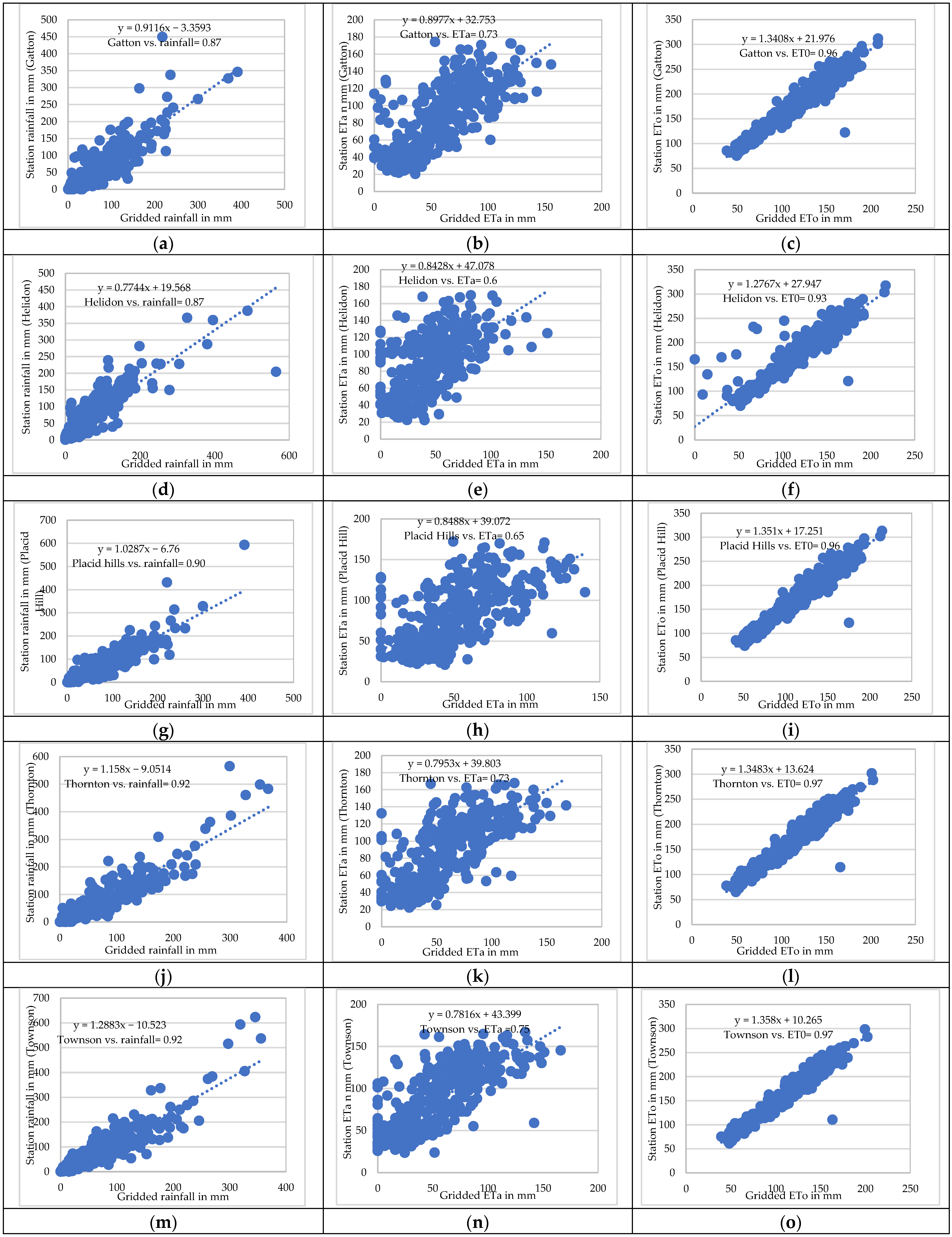
| Station | Variable mm | R2 % | Pearson’s Correlation | RMSE mm/Month | Bias | MBias |
|---|---|---|---|---|---|---|
| Gatton | P | 0.76 | 0.87 | 45.38 | 1.14 | 0.16 |
| ETa | 0.53 | 0.73 | 49.96 | −34.07 | 0.15 | |
| ETo | 0.94 | 0.96 | 83.73 | −71.33 | 0.28 | |
| Placid Hills | P | 0.82 | 0.90 | 48.35 | −4.63 | 0.16 |
| ETa | 0.42 | 0.65 | 54.34 | −38.45 | 0.13 | |
| ETo | 0.94 | 0.96 | 83.15 | −69.19 | 0.28 | |
| Thornton | P | 0.84 | 0.92 | 44.09 | −9.04 | 0.17 |
| ETa | 0.54 | 0.73 | 51.47 | −35.77 | 0.14 | |
| ETo | 0.94 | 0.97 | 80.25 | −64.27 | 0.27 | |
| Townson | P | 0.84 | 0.92 | 57.10 | −19.70 | 0.17 |
| ETa | 0.56 | 0.75 | 53.02 | −39.15 | 0.14 | |
| ETo | 0.95 | 0.97 | 77.29 | −62.01 | 0.26 | |
| Upper Tenthill | P | 0.80 | 0.89 | 41.93 | −0.17 | 0.16 |
| ETa | 0.35 | 0.59 | 58.56 | −45.15 | 0.12 | |
| ETo | 0.94 | 0.97 | 81.23 | −65.86 | 0.28 | |
| West Haldon | P | 0.82 | 0.90 | 38.97 | −4.07 | 0.16 |
| ETa | 0.51 | 0.72 | 49.14 | −33.76 | 0.15 | |
| ETo | 0.95 | 0.97 | 73.13 | −56.93 | 0.29 | |
| Whitestone | P | 0.83 | 0.91 | 37.53 | 3.14 | 0.16 |
| ETa | 0.54 | 0.74 | 45.23 | −30.51 | 0.15 | |
| ETo | 0.944 | 0.97 | 74.33 | −62.85 | 0.28 |
| Test | Statistical Tests | p-Value | Test Statistic | Critical Values | Test Result | ||
|---|---|---|---|---|---|---|---|
| SL = 0.1 | SL = 0.05 | SL = 0.01 | |||||
| Placid Hills | |||||||
| Trend detection | Mann–Kendall | 0.028 | −2.2 | 1.645 | 1.960 | 2.576 | H0 rejected at 5% |
| Global climate dataset corresponding to Placid Hills | |||||||
| Trend detection | Mann–Kendall | 0.011 | −2.5 | 1.645 | 1.960 | 2.576 | H0 rejected at 5% |
| Townson | |||||||
| Trend detection | Mann–Kendall | 0.009 | −2.62 | 1.645 | 1.960 | 2.576 | H0 rejected at 1% |
| Global climate dataset corresponding to Townson | |||||||
| Trend detection | Mann–Kendall | 0.016 | −2.41 | 1.645 | 1.960 | 2.576 | H0 rejected at 5% |
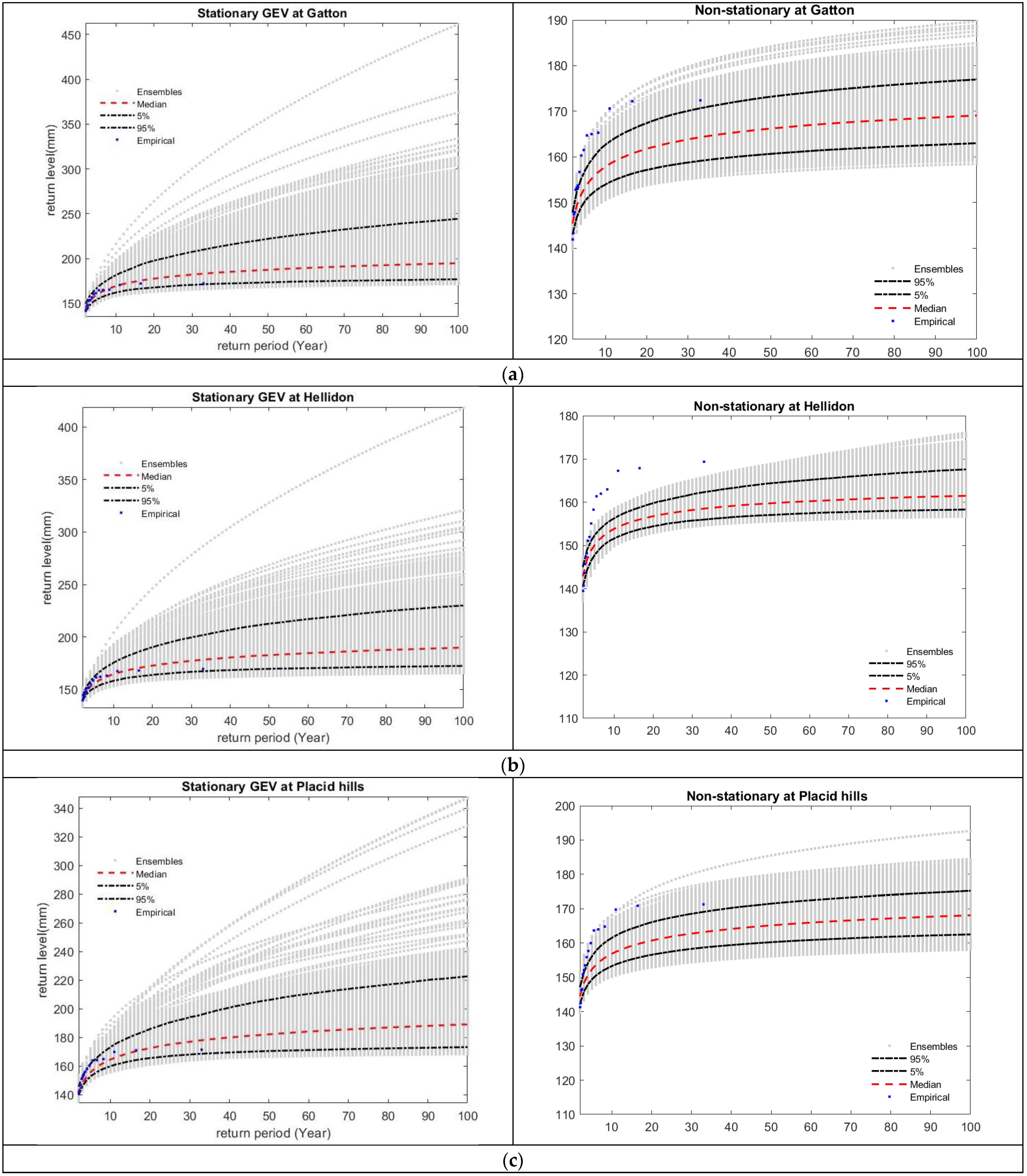
| Rainfall | Rainfall | |||
|---|---|---|---|---|
| Return Period | Station | ERA5 Data | ||
| Gatton | Stationary | Non-Stationary | Stationary | Non-Stationary |
| 10 | 312.64 | 324.47 | 279.35 | 282.12 |
| 20 | 379.38 | 402.04 | 325.41 | 328.86 |
| 50 | 472.53 | 520.23 | 388.93 | 394.75 |
| 100 | 550.98 | 624.97 | 441.30 | 450.77 |
| Helidon | ||||
| 10 | 339.96 | 336.66 | 292.61 | 325.507 |
| 20 | 437.19 | 436.11 | 343.12 | 393.58 |
| 50 | 596.99 | 606.25 | 417.67 | 492.67 |
| 100 | 748.07 | 765.74 | 478.62 | 575.84 |
| Placid Hills | ||||
| 10 | 310.52 | 323.20 | 267.89 | 298.30 |
| 20 | 371.52 | 387.83 | 305.19 | 406.05 |
| 50 | 467.35 | 491.09 | 354.20 | 624.46 |
| 100 | 560.60 | 583.60 | 390.19 | 874.67 |
| Townson | ||||
| 10 | 434.12 | 419.51 | 289.18 | 303.4 |
| 20 | 528.48 | 513.25 | 344.46 | 365.64 |
| 50 | 670.93 | 657.57 | 424.26 | 460.33 |
| 100 | 796.57 | 788.64 | 493.24 | 544 |
| Whitestone | ||||
| 10 | 311.75 | 325.49 | 285.94 | 285.94 |
| 20 | 370.14 | 390.83 | 340.92 | 340.92 |
| 50 | 452.33 | 479.13 | 422.21 | 422.21 |
| 100 | 512.60 | 546.52 | 499.93 | 499.93 |
| Water Storage | Water Storage | |||
|---|---|---|---|---|
| Return Period | Based on Station | Based on ERA5 Data | ||
| Gatton | Stationary | Non-Stationary | Stationary | Non-Stationary |
| 10 | 100.71 | 100.71 | 95.45 | 108.70 |
| 20 | 144.89 | 144.89 | 126.97 | 142.55 |
| 50 | 202.65 | 202.65 | 168.84 | 188.3 |
| 100 | 247.64 | 247.64 | 202.44 | 224.80 |
| Helidon | ||||
| 10 | 133.93 | 133.93 | 132.96 | 132.96 |
| 20 | 196.26 | 196.26 | 156.91 | 156.91 |
| 50 | 286.70 | 286.70 | 195.64 | 195.64 |
| 100 | 363.34 | 363.34 | 224.83 | 224.83 |
| Placid Hills | ||||
| 10 | 120.79 | 120.79 | 113.70 | 113.70 |
| 20 | 179.07 | 179.07 | 136.92 | 136.92 |
| 50 | 255.67 | 255.67 | 163.25 | 158.23 |
| 100 | 316.06 | 316.06 | 180.55 | 176.99 |
| Thornton | ||||
| 10 | 165.76 | 165.76 | 110.55 | 110.55 |
| 20 | 233.13 | 233.13 | 137.04 | 137.04 |
| 50 | 328.51 | 328.51 | 174.03 | 174.03 |
| 100 | 415.159 | 415.159 | 199.66 | 199.66 |
| Townson | ||||
| 10 | 197.20 | 197.20 | 97.80 | 97.80 |
| 20 | 256.35 | 256.35 | 136.77 | 136.77 |
| 50 | 343.19 | 343.19 | 193.38 | 193.38 |
| 100 | 411.08 | 411.08 | 241.17 | 241.17 |
| Whitestone | ||||
| 10 | 99.57 | 106.32 | 96.92 | 96.92 |
| 20 | 156.79 | 164.97 | 147.03 | 147.03 |
| 50 | 244.30 | 258.30 | 231.33 | 231.33 |
| 100 | 321.33 | 344.60 | 314.13 | 314.13 |
Disclaimer/Publisher’s Note: The statements, opinions and data contained in all publications are solely those of the individual author(s) and contributor(s) and not of MDPI and/or the editor(s). MDPI and/or the editor(s) disclaim responsibility for any injury to people or property resulting from any ideas, methods, instructions or products referred to in the content. |
© 2023 by the authors. Licensee MDPI, Basel, Switzerland. This article is an open access article distributed under the terms and conditions of the Creative Commons Attribution (CC BY) license (https://creativecommons.org/licenses/by/4.0/).
Share and Cite
Pakdel, H.; Paudyal, D.R.; Chadalavada, S.; Alam, M.J.; Vazifedoust, M. A Multi-Framework of Google Earth Engine and GEV for Spatial Analysis of Extremes in Non-Stationary Condition in Southeast Queensland, Australia. ISPRS Int. J. Geo-Inf. 2023, 12, 370. https://doi.org/10.3390/ijgi12090370
Pakdel H, Paudyal DR, Chadalavada S, Alam MJ, Vazifedoust M. A Multi-Framework of Google Earth Engine and GEV for Spatial Analysis of Extremes in Non-Stationary Condition in Southeast Queensland, Australia. ISPRS International Journal of Geo-Information. 2023; 12(9):370. https://doi.org/10.3390/ijgi12090370
Chicago/Turabian StylePakdel, Hadis, Dev Raj Paudyal, Sreeni Chadalavada, Md Jahangir Alam, and Majid Vazifedoust. 2023. "A Multi-Framework of Google Earth Engine and GEV for Spatial Analysis of Extremes in Non-Stationary Condition in Southeast Queensland, Australia" ISPRS International Journal of Geo-Information 12, no. 9: 370. https://doi.org/10.3390/ijgi12090370
APA StylePakdel, H., Paudyal, D. R., Chadalavada, S., Alam, M. J., & Vazifedoust, M. (2023). A Multi-Framework of Google Earth Engine and GEV for Spatial Analysis of Extremes in Non-Stationary Condition in Southeast Queensland, Australia. ISPRS International Journal of Geo-Information, 12(9), 370. https://doi.org/10.3390/ijgi12090370