Abstract
Agricultural intensification practices have been adopted in the Brazilian savanna (Cerrado), mainly in the transition between Cerrado and the Amazon Forest, to increase productivity while reducing pressure for new land clearing. Due to the growing demand for more sustainable practices, more accurate information on geospatial monitoring is required. Remote sensing products and artificial intelligence models for pixel-by-pixel classification have great potential. Therefore, we developed a methodological framework with spectral indices (Normalized Difference Vegetation Index (NDVI), Normalized Difference Water Index (NDWI), and Soil-Adjusted Vegetation Index (SAVI)) derived from the Harmonized Landsat Sentinel-2 (HLS) and machine learning algorithms (Random Forest (RF), Artificial Neural Networks (ANNs), and Extreme Gradient Boosting (XGBoost)) to map agricultural intensification considering three hierarchical levels, i.e., temporary crops (level 1), the number of crop cycles (level 2), and the crop types from the second season in double-crop systems (level 3) in the 2021–2022 crop growing season in the municipality of Sorriso, Mato Grosso State, Brazil. All models were statistically similar, with an overall accuracy between 85 and 99%. The NDVI was the most suitable index for discriminating cultures at all hierarchical levels. The RF-NDVI combination mapped best at level 1, while at levels 2 and 3, the best model was XGBoost-NDVI. Our results indicate the great potential of combining HLS data and machine learning to provide accurate geospatial information for decision-makers in monitoring agricultural intensification, with an aim toward the sustainable development of agriculture.
1. Introduction
The Brazilian tropical savanna (Cerrado) covers an area of more than 200 million hectares in the central region of Brazil and is the largest food, fiber, and agro-energy producer in the country, mainly through the production of soybean (Glycine max L.), maize (Zea mays L.), cotton (Gossypium L.), sugarcane (Saccharum officinarum L.), fruit, and cattle beef [1]. This region stands out due to its agricultural intensification practices, mainly in the transition zone between the Cerrado and Brazilian Amazon in Mato Grosso State [2,3]. Agricultural intensification involves more applications of pesticides, herbicides, and chemical fertilizers and the adoption of irrigation to increase productivity [4,5]. Another method of intensification is the use of a double cropping system in which farmers plant short-cycle varieties of soybean so that they still have enough time to plant a second crop during the same rainy season [6,7,8,9].
From a remote sensing perspective, the monitoring of the Cerrado’s agricultural intensification, especially farms involving double or even triple cropping systems, is challenging due to its high spatial variability, spectral similarity among some crops, different planting dates, and presence of cloud coverage, especially during the six-month rainy season (October to March) [10]. However, with the recent launch of several orbital platforms carrying different sensors operating in distinct image acquisition modes, there are new possibilities to monitor such intensification, expansion, and retraction [9,11,12,13,14].
Agricultural monitoring in the Brazilian savanna has been carried out mainly using products derived from high temporal resolution sensors, such as the Moderate Resolution Imaging Spectroradiometer (MODIS), especially vegetation indices with a 16-day temporal resolution and a spatial resolution of 250 m [10,15,16,17]. However, the spatial resolution of the MODIS prevents a more precise analysis of the pixel-by-pixel mapping of agricultural intensification since there is an impact of landscape fragmentation on the performance of models with coarse-resolution images, limiting their application for large-scale agriculture [10,15]. Therefore, to overcome this disadvantage, it is appropriate to use products with higher spatial resolution, for example, the Harmonized Landsat Sentinel-2 (HLS), proposed by NASA, which considers the combination of the Landsat Operational Land Imager (OLI) and the Sentinel-2 Multispectral Instrument (MSI) satellites and improves the number of overpasses with a spatial resolution of 30 m [18].
Previous studies have massively focused on the use of the Normalized Difference Vegetation Index (NDVI) and Enhanced Vegetation Index (EVI) to map intensive cropping systems [8,10,15,16,17,19]. Thus, it becomes relevant to diversify vegetation indices, which can translate into statistical gains and, consequently, into better discrimination of different types of crops. The NDVI and EVI have the same purpose, which is to evaluate the vegetation’s vigor; therefore, combining these with indices measuring moisture content, such as the Normalized Difference Water Index (NDWI), can help in the discrimination of different crops, especially irrigated crops, or the use of indices capable of eliminating the soil response in the reflectance recorded by the sensor, such as the Soil-Adjusted Vegetation Index (SAVI), could increase the ability to discriminate sparse crops from exposed soil. Previous studies found that index diversification, especially the addition of shortwave infrared (SWIR) wavelengths, improves the separability of crop types [14,20,21].
Therefore, this study aimed to evaluate the potential of three different spectral indices derived from HLS products, namely NDVI, NDWI, and SAVI, to map agricultural intensification and crop types (corn, cotton, beans, and other crops cultivated in the second crop season) in an area with very high production. To the best of our knowledge, there is no study using these data to assess agricultural intensification in the Brazilian savanna. The performance of three ML algorithms was also assessed: one that has been previously used in related studies, i.e., the Random Forest (RF), and two that have not yet been tested in the analysis of agricultural intensification: an Artificial Neural Network (ANN), an algorithm that has already proven useful for several purposes in an agricultural context [22], including crop mapping [23], and Extreme Gradient Boosting (XGBoost), a relatively recent algorithm that has shown superior performance in classifying crop types when confronted with multiple ML classifiers [21,24,25].
Based on this methodological structure, we intend to answer the following scientific questions. (i) Is the improved temporal resolution made possible by HLS data sufficient to capture phenological variations and discriminate between different types of crops and cropping practices? (ii) Does the diversification of spectral indices improve the accuracies in mapping intensification and crop types? (iii) Can the use of an ANN and XGBoost provide even more robust mapping of intensification and crop types than RF?
2. Materials and Methods
2.1. Study Area
The study area corresponds to the municipality of Sorriso (central coordinates: 55°40′41.6″ W and 12°44′30.7″ S), located in the central part of Mato Grosso State, Brazil, in a transitional zone between Cerrado and the tropical rainforest (Figure 1). This municipality is officially named the “national capital of agribusiness” (Federal Law n. 12.724, 16 October 2012) because of its highly mechanized production of rainfed grains for export [26]. The topography is predominantly composed of lowlands (altitude varying between 300 m and 470 m); the soil texture is favorable for extensive grain production (clayey and medium textures) and the rainfall is sufficient for double cropping with low climatic risk [27,28].
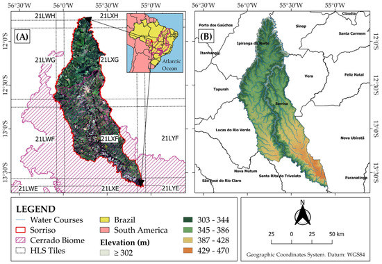
Figure 1.
(A) Location of the study area, which corresponds to the municipality of Sorriso in the Brazilian tropical savanna (Cerrado) and Mato Grosso State, Brazil. (B) Digital elevation model of the study area obtained from Copernicus DEM GLO-30: Global 30 m using the Google Earth Engine. Sources: territorial boundaries [29]; Cerrado boundaries [30]; HLS tiles [31]; water courses [32].
In 2021, the Sorriso municipality harvested more than 1.2 million ha of temporary crops, mostly from double cropping systems (Table 1), following the same trend as Mato Grosso State. In this state, in the 2000–2001 crop growing season, double cropping systems were adopted in about 6% of the total temporary croplands [2]. Nowadays, it is the most common production system, estimated at 8.4 million ha in 2016 [15]. The expansion of irrigation practices, mostly based on center pivots, also contributed to the intensification. For example, in 2000, there were 14 center pivots installed in Sorriso, which increased to 173 in 2019 [32].

Table 1.
Total area harvested in the municipality of Sorriso, Mato Grosso State, Brazil, in the 2020−2021 crop growing season.
2.2. Remote Sensing Data Sets
This study was based on spectral indices derived from HLS images processed by spatial, temporal, and band filters [18]. The HLS Landsat OLI images converted into surface reflectance and top-of-atmosphere (TOA) brightness data (HLS.L30) and the HLS Sentinel-2 MSI images converted into surface reflectance (HLS.S30) were downloaded from NASA’s Application for Extracting and Exploring Analysis Ready Samples (AρρEEARS) data access platform. All available surface reflectance data from red (R) (640–670 nm), near-infrared (NIR) (850–880 nm), and shortwave infrared (SWIR) (1570–1650 nm) wavelengths were acquired within the limits of the study area at a 30 m spatial resolution between September 2021 and August 2022. Whenever HLS.L30 and HLS.S30 overpasses coincided, we selected the latter.
The HLS data set is produced by NASA through the following processing chain: atmosphere correction, spatial co-registration, Bidirectional Reflectance Distribution Function (BRDF) normalization, and bandpass adjustment [18]. The atmosphere correction involves the use of the Land Surface Reflectance Code (LaSRC) based on the 6S radiative transfer code [34]. The Automated Registration and Orthorectification Package [35] is used to perform the spatial co-registration between Landsat OLI and Sentinel-2 MSI images to the same reference per tile. The c-factor technique and global coefficients are used to reduce the sun sensor geometry effects by estimating BRDF and Nadir BRDF-adjusted reflectance with scattering models [36,37]. Finally, differences between MSI and OLI equivalent bands are adjusted by linear fit using slope and offset coefficients generated with 160 global hyperion scenes [18].
The images were additionally processed using R statistical software [38] to apply the scale factor (0.0001), cloud masking, gap filling, and generation of the spectral indices. Initially, the original HLS quality assessment band (Fmask) removed pixels flagged with cloud, cloud shadow, cloud shadow adjacencies, and water. Therefore, only the integer values 64, 128, and 192, representing clean pixels and the medium aerosol limit, were kept. It was necessary to use pixels with this limit to reduce the amount of data lost since Fmask tends to overestimate aerosol levels (see the users’ guide [39] for full details on HLS cloud masking). HLS.L30 and HLS.S30 images were stacked, and the gaps created in the multispectral time series by the cloud masks were filled by simple linear interpolation across layers using the “raster” package [40].
Finally, we calculated the following spectral indices: the NDVI, NDWI, and SAVI (see equations in Table 2. In general, agricultural intensification studies are carried out using MODIS products, so the EVI and NDVI are readily available. The selected spectral indices capture the phenological dynamics of crop cycles well [8,10,41]. The NDVI is the most popular vegetation index used for mapping land use and land cover (LULC) and a wide range of other applications since it is related to photosynthetic activity [42]. The SAVI is less sensitive to soil background effects than the NDVI and has proven to be a valuable variable for agriculture mapping in previous studies (e.g., Parreiras et al. [14]). The NDWI considers a SWIR band that is sensitive to the leaf water content and biochemical component variation among several vegetation types, which can be an advantage for differentiating between classes with similar spectral responses in the NIR and red domains [43]. The combined use of the three spectral indices was also evaluated, henceforth referred to as All VI.
Table 2.
Equations and citations of the spectral indices used in the study.
2.3. Methodological Approach
The main steps of our methodological approach were (i) fieldwork for the selection of samples; (ii) creation of synthetic samples; (iii) elaboration of the hierarchical classification scheme; (iv) obtaining the HLS data set and generating spectral indices; (v) training ML algorithms for classification; and (vi) accuracy assessment (Figure 2).
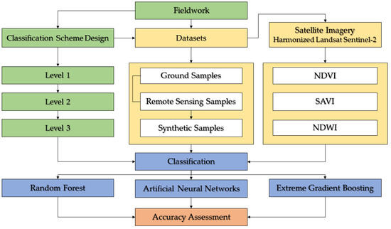
Figure 2.
Workflow showing the main steps and variables for the machine learning classifications performed in this study. NDVI = Normalized Difference Vegetation Index; SAVI = Soil-Adjusted Vegetation Index; and NDWI = Normalized Difference Water Index.
To assess agriculture intensification and second-season crop types in Sorriso, we conducted a field campaign from 6 to 9 June 2022, which corresponded to the end of the second crop season as well as the start of the third season for irrigated crops. We gathered 318 randomly distributed ground samples with the support of the AgroTag mobile application developed by Embrapa [47]. AgroTag provides structured queries to allow the storage of detailed, georeferenced ground sample information, as well as panoramic and nadir field photos (Figure 3).
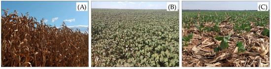
Figure 3.
Field panoramic photos obtained in early June 2022 showing the general stage of development of corn (A), cotton as the second crop (B), and irrigated beans as the third crop (C).
Based on field information, a hierarchical classification scheme was adopted to discriminate the main LULC classes found in Sorriso (Figure 4). Initially, we created a mask to distinguish areas with vegetation, including natural and agricultural land, and areas without vegetation. Data from the MapBiomas Project [48,49] were used to delineate the pixels corresponding to all non-vegetated areas (urban, mining, water, and others). Highways were excluded based on the cartographic database from the Instituto de Terras de Mato Grosso at a 1:100,000 scale [50]. A 30 m buffer was used to represent road width and consequently carry out the extraction. From this procedure, all non-vegetated pixels were masked out, and level 1 classification was performed on the remaining vegetated areas.
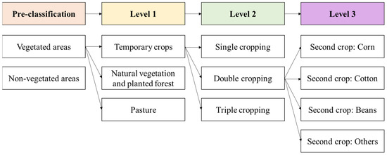
Figure 4.
Hierarchical classification scheme adopted to represent the main agricultural uses and vertical intensification in Sorriso, Mato Grosso State, Brazil, in the 2021−2022 crop growing season.
In the level 1 classification procedure, we differentiated the study area into areas containing (i) temporary crops, (ii) natural vegetation and planted forests (or silviculture), and (iii) pasturelands. Planted forests were mapped together with the natural vegetation because of their low occurrence in the study area. Then, we divided the temporary crops based on the number of cycles, including single, double, or triple cropping (level 2). Sugarcane was classified as a single crop, while triple cropping was exclusively observed in center-pivot irrigation systems, mainly with beans as the third-season crop. Although all triple cropping was related to center pivots, not all center pivots were related to triple cropping. Finally, at level 3, double cropping areas were categorized into corn, cotton, beans, and other crops, that is, mainly sorghum and millet. These crops were grown in the second season, mainly following the soybean harvest.
Even though there is substantial progress regarding satellite image availability and non-parametric, supervised classification algorithms, the acquisition of balanced ground sample data sets is still a challenge in LULC mapping procedures. The imbalance of reference data sets significantly affects image classification [51]; however, the sampling must be representative of the occurrence of LULC classes [52]. In this study, we faced a bias toward the high occurrence of double cropping with corn as a second crop. It represented approximately 50% of the total number of samples.
Therefore, additional samples of natural vegetation, pastures, planted forests, sugarcane, and triple cropping were collected remotely using a high-resolution Norway’s International Climate and Forest Initiative (NICFI) PlanetScope monthly mosaic (Imagery © 2022 Planet Labs Inc., San Francisco, CA, USA), an HLS 30 m RGB false color composite of bands 8, 4, and 3, and the temporal NDVI profile from the MODIS sensor available in the SatVeg platform developed by Embrapa Agricultura Digital [53]. The elements and interpretation keys that guided the sample selection are described, with examples, in the Supplementary Materials. Table 3 summarizes the final number of samples used for further ML classification.
Table 3.
The number of ground and remotely acquired samples for each land use and land cover (LULC) class for the hierarchical classification scheme.
At levels 2 and 3, the method known as the Synthetic Minority Oversampling Technique (SMOTE) was used to increase the number of samples of minor classes, that is, classes with less than 15% occurrence in a specific level, by generating synthetic samples. The SMOTE is the most popular algorithm to deal with imbalance problems in LULC classification [44], and it was implemented using the “scutr” package [54] in R software, version 4.2.2 [38]. Before creating synthetic samples, we carried out a quality control process to check the correctness of every ground sample point with HLS color compositions from the same period of the field visit. Table 4 summarizes the final number of samples used for further ML classification at levels 2 and 3, while Figure 5 exhibits the spatial distribution of the sampling points used in each level.
Table 4.
The number of primary (acquired in situ or remotely) and synthetic samples generated by the Synthetic Minority Oversampling Technique (SMOTE) for each class at classification levels 2 and 3.
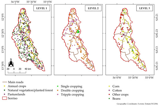
Figure 5.
Spatial distribution of the samples used in each classification level and main road network obtained from INTERMAT (2023).
The methodological structure was set up using “Caret” and “randomForest” packages [55,56] in the R environment [38]. We considered the samples of LULC classes as the y variables to be predicted and the satellite image time series database (NDVI, SAVI, and NDWI) as the x predictor variables. We evaluated the following supervised classification algorithms: XGBoost [57], ANN [58] (both available in the Caret package), and RF [56] (using the randomForest package). We used a 70%/30% ratio to split the data sets into training and test subsets for level 1. Due to the smaller number of observations in some classes, a ratio of 60%/40% was adopted for levels 2 and 3.
RF is a decision tree model that uses the bootstrap method. More specifically, it creates several sets of trees with different variables to decrease the correlation between the trees to avoid overfitting in the predictions. Each tree presents a prediction, and the final prediction is given by considering the voting rules for each class mapped in the trees [59]. The main RF hyperparameters to be adjusted are the mtry, i.e., the number of features drawn for the split, and the number of trees in the forest (nTree). XGBoost is also a model based on decision trees; however, while RF uses the bootstrap method, XGBoost works with boosting, in which trees with weak predictions are improved over time. The final classification is based on improving trees through iterative processes [57]. The XGBoost hyperparameters to be adjusted are nrounds, lambda, and alpha.
The ANN is a model inspired by the neurological behavior of the human brain. The neural network is composed of layers, which comprise prediction phases. In the first phase, there is the input layer, responsible for presenting the neural network with the training variables and their behavior patterns. The second phase is where all the processing occurs, i.e., the model training stage, known as hidden layers. Finally, there is the output layer, where the result of the prediction is provided [58]; in our case, the prediction is the agricultural intensification classes. Size and Decay are the hyperparameters in the ANN model. All models were trained and the hyperparameters were automatically tuned through a grid search cross-validation with 5 folds and 10 repetitions.
To assess the model performances, we considered the confusion matrices and their corresponding metrics of overall accuracy (OA), which refers to the rate of correct answers in relation to the total number of samples, and the kappa index, which refers to the degree of agreement between the classification results and the reference data. Additionally, to assess class accuracies, we also considered errors of omission (OEs; samples that were not classified according to the reference classes in the rows of the matrix) and commission errors (CEs; reference samples misclassified as belonging to other classes in the columns) [60].
The model results were subjected to analysis of variance (ANOVA) to assess possible statistical differences after the Shapiro–Wilk normality test. The importance of model variables was evaluated using the VarImp function. For the RF algorithm, the importance was given by the Mean Decrease Accuracy (MDA), while for XGBoost and ANN, we considered the relative importance, that is, Overall%. MDA measures the impact of changing the variable of interest on model accuracy. In the Overall%, the importance values were scaled from 0 to 100, with the least important variables close to 0 and the most explanatory close to 100. The results of this study were also analyzed in comparison to similar studies, mainly those carried out in the Brazilian savanna, to identify the advances brought by the proposed approach.
3. Results
3.1. Data Availability and Cloud Cover
Tropical areas are severely affected by cloud presence, especially during the rainy season, creating challenges for the monitoring of crop development with optical remote sensing, i.e., crop mapping [61]. We found an average cloud cover of 57.5% over Sorriso between September and March (rainy season) and 11% between April and August (dry season) (Figure 6). The median gap between valid observations was five days in the rainy season and three days in the dry season. Among the 102 overpasses (some dates that were entirely cloud-covered were disregarded), 60 were from Sentinel-2 (HLS.S30) and 42 were from Landsat 8/9 (HLS.L30). However, the total number of observations at each pixel within the study period was 81 (60 HLS.S30 + 21 HLS.L30), considering the different overpasses between paths/rows 227/68 and 226/69 from Landsat products.
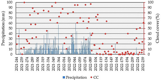
Figure 6.
Daily precipitation (mm) obtained from the Climate Hazards Group InfraRed Precipitation with Station (CHIRPS). Data are available in the Google Earth Engine (GEE) platform, and average cloud cover (%) was estimated using Harmonized Landsat Sentinel-2 images in the municipality of Sorriso, Mato Grosso State, Brazil.
3.2. Accuracy Assessment and Importance of Variables
Table 5, Table 6 and Table 7 show the OA and kappa index for all three ML models at levels 1, 2, and 3, respectively. The performances were above 93% in terms of OA and above 0.85 in terms of kappa index, regardless of the ML classifier. These performances were similar according to ANOVA (Supplementary Materials) without any statistical differences (p > 0.05). RF associated with the NDVI performed better than the other models (OA = 95%; kappa index = 0.93) at level 1, while XGBoost, also associated with the NDVI, performed better at levels 2 and 3. Considering the combination of all indices (All VI) at level 1, RF performed better. At level 2, the ANN had a better statistical performance, while at level 3, XGBoost and the ANN performed similarly. Although it could be expected that merging the three indices would improve performance, this was not the case in this study.
Table 5.
Classification results by RF, ANN, and XGBoost, trained with the NDVI, NDWI, SAVI, and All VI at level 1.
Table 6.
Classification results by RF, ANN, and XGBoost, trained with the NDVI, NDWI, SAVI, and All VI at level 2.
Table 7.
Classification results by RF, ANN, and XGBoost, trained with the NDVI, NDWI, SAVI, and All VI at level 3.
Table 8, Table 9 and Table 10 show the confusion matrices, with the OE, CE, OA(%), and the kappa index of the three best ML models for levels 1, 2, and 3, respectively. Following the behavior of global metrics, the specific statistics by LULC classes also confirmed the good performance of the methodological framework, mainly with OE values ranging from 0 to 17% and CE values from 0 to 23% (all confusion matrices are shown in the Supplementary Materials).
Table 8.
Confusion matrix and accuracy metrics for the best level 1 model (Random Forest and the NDVI).
Table 9.
Confusion matrix and accuracy metrics for the best level 2 model (Extreme Gradient Boost and the NDVI).
Table 10.
Confusion matrix and accuracy metrics for the best level 3 model (Extreme Gradient Boost and the NDVI).
Figure 7 shows the ranking of importance of the variables that best explained the variations of the LULC classes selected in the training phase in terms of overall percentage and MDA. Our data sets were composed of 102 overpasses; however, we selected the 20 most important ones for further analysis, and at all levels, more than 80% of the most relevant images were from the dry period (April to September).
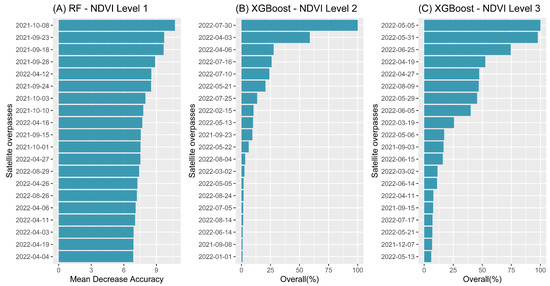
Figure 7.
Ranking of importance for the best models by spectral index at levels 1, 2, and 3. RF = Random Forest; XGBoost = Extreme Gradient Boosting; NDVI = Normalized Difference Vegetation Index.
3.3. Machine Learning-Based Digital Classification Results
We selected the ML models associated with spectral indices with the highest metrics by hierarchical levels (Table 5, Table 6 and Table 7) for the spatialization of agricultural intensification mapping (Figure 8). At level 1, we found that most of the municipality was covered by temporary crops (57%), followed by natural vegetation and planted forests (29%) and pastures (11%) (Figure 8). This reinforces the fact that the municipality of Sorriso is considered the “national capital of agribusiness”. At level 2, we found a predominance of double cropping (96%), with less territorial expression of single cropping (~1%) and triple cropping (~3%). At level 3, our model (XGBoost associated with the NDVI) mapped corn as the main crop cultivated in the second season (439,304 ha). Cotton was the second largest crop (51,958 ha), followed by other crops, mainly millet and sorghum. Corn was the main crop in the double cropping system in the municipality of Sorriso and also in Mato Grosso State [15] and other regions of the Brazilian savanna [8,9].
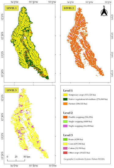
Figure 8.
Final maps using the most accurate models at levels 1 (RF-NDVI), 2 (XGBoost-NDVI), and 3 (XGBoost-NDVI).
4. Discussion
4.1. Accuracy Assessment and Importance of Variables
The adoption of sustainable agriculture requires accurate mapping and monitoring procedures to discriminate between different production systems [10,62,63,64]. Hence, the use of ML models coupled with spectral indices for this purpose has grown worldwide [42,65]. In our study, we used ANNs, RF, and XGBoost coupled with the NDVI, NDWI, and SAVI and four crop levels validated with ground, remote, and synthetic samples. Based on this approach, we obtained mapping accuracies between 85% and 99%, suggesting high reliability of the models.
RF and XGBoost, which are decision tree models, were the most efficient models at the three levels analyzed. This pattern of higher performances for decision tree models agrees with the previous studies carried out in other regions, both in agricultural [10,23,66] and environmental contexts [67]. RF and XGBoost have a robust methodological architecture related to their training, bootstrap, and boosting methods [57,59]. In RF, the bootstrap can create several subgroups of samples during the construction of trees. These samples are divided randomly, with the aim of decreasing the correlation between trees [55]. These characteristics make RF a powerful model for classifying complex land uses [59], which is the case in the Brazilian savanna [8,9,14,15,16]. As mentioned previously, XGBoost uses boosting logic, in which the model trains several trees and the trained trees with low performance are optimized and sequentially improved [57]. Although agricultural classes are very heterogeneous, boosting provides a high potential for separability, as seen in other studies [68].
The ANN did not present a significant difference (p-value > 0.05); in general, it produced lower metrics compared to the other models. Studies applying an ANN for LULC classification found that when compared with other models, especially the ones based on decision trees, the ANN tends to present a lower performance [23,24,25,26,27,28,29,30,31,32,33,34,35,36,37,38,39,40,41,42,43,44,45,46,47,48,49,50,51,52,53,54,55,56,57,58,59,60,61,62,63,64,65,66], which can be associated with its limited number of hidden layers. The use of convolutional and recurrent neural networks (CNNs and RNNs, respectively) has been suggested to solve this ANN problem [69]. However, the computational cost can be high, mainly when the time series of high-resolution images are involved.
Our estimated data for corn presented a difference of 104,696 ha (−19%) in relation to the Municipal Agricultural Production (PAM) data provided by the Brazilian Institute for Geography and Statistics [33]. As PAM is based on interviews with a sample of producers and technicians, it is more suitable for comparisons encompassing large areas or long time periods, as carried out in [70]. Thus, differences between crop areas mapped by remote sensing and IBGE at the municipal scale were already expected.
Considering the 20 most important variables selected by the models, there was a predominance of dry season images (>80%). This suggests that using images in this season is more efficient in distinguishing areas of natural vegetation, pastures, and crops. This season allows high spectral contrast between pastures and natural vegetation/planted forests (or silviculture) since pastures become dry quickly [14]. Agricultural crops are certainly associated with the fact that their phenological development is expected to occur in the transition to the dry season, that is, between April and September.
4.2. Crop Calendar and Vegetation Index Temporal Signature
According to the Agricultural Climate Risk Zoning (ZARC) produced by the Brazilian Ministry of Agriculture and Livestock, the recommended sowing dates for corn as the second crop in Sorriso following soybean harvest are between February and March [71]. The HLS-NDVI time series was able to capture this trend. The NDVI values started to increase at the beginning of February, reaching a peak in early April (Figure 9, level 3). In general, the cotton sowing period as the second crop in Sorriso occurs right after the soybean harvest, up until February, and crop’s physiological maturation takes about 170 days [72]. This aspect is represented by the larger peak of the NDVI values in Figure 9 from early April to early June. The amplitude of the beans cycle depends on the crop cultivar and production system, but it usually ranges from 75 days to 95 days in Mato Grosso [73]. The NDVI values for beans as second crops started to increase in early March and then began decreasing until early June. Beans can be cultivated in double cropping systems following soybeans, with sowing dates between January and March, or under irrigation systems in the third season, between May and June.
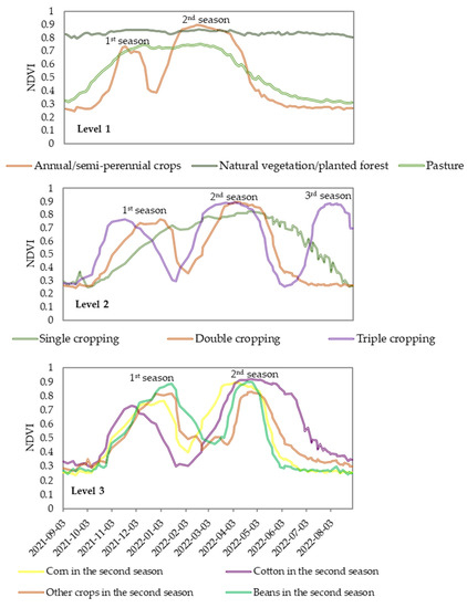
Figure 9.
Median HLS NDVI time series for levels 1, 2, and 3 between September 2021 and August 2022, indicating the occurrence of the first, second, and third crop seasons for agricultural areas with more than one cycle. Level 3 exhibits the entire crop season NDVI signature; however, only the second season profiles refer to the target crops: corn, cotton, beans, or other crops.
During the fieldwork conducted in early June 2022, most of the corn fields were already harvested; in the cotton fields, the bolls were fully open or starting senescence; beans as a second crop were also harvested, although there were some bean plantations presenting primary leaves in center pivots, starting the third crop season. All these patterns can also be observed in Figure 9. These spectral behaviors agree with the previous works carried out in the Cerrado biome [8,10], showing that spectral indices can capture these seasonal climatic conditions, which are crucial for mapping agricultural intensification and crop types.
4.3. Advances and Limitations
Previous studies have mapped agricultural intensification in Brazil, particularly in the Cerrado region; for example, agricultural intensification in the state of Mato Grosso was mapped using a MODIS time series with a coarse resolution [10,15,16,17,19]. More recent studies have employed improved spatial resolution data, such as Landsat [8] and PlanetScope monthly mosaics [9], in the states of Bahia (northeast of Brazil) and Goiás (central part of Brazil), respectively. ML algorithms such as RF [8,9,16], Decision Tree Classifiers [10,17], and Support Vector Machines [15,16] have been increasingly used, resulting in models with high overall accuracy (>80%), particularly the decision tree-based models.
The EVI and NDVI, either raw or transformed into derivatives, such as phenometrics (start, end, and length of the season, among others), have been widely used as explanatory variables for agricultural intensification mapping [8,10,16]. This study brings some important contributions, including the use of HLS data, a multisensor approach still underexplored in Brazil [14] that provided a time series with a median temporal resolution of up to 4.5 days. Although [8,9] mapped double cropping systems using 30 m and 4.77 m spatial resolution satellite images, the temporal resolution was limited to 8 and 30 days, respectively.
As mentioned, high cloud cover in tropical regions affects agricultural mapping through optical remote sensing. Prudente et al. [61] showed that the frequency of clouds over the central portion of Mato Grosso State usually exceeded 70% between December and February, making it challenging to monitor crops, such as soybean and corn, during the summer. In this study, the average cloud cover in the rainy season was 57.5%, varying between 10% and 97% depending on the day. Therefore, answering the first question in our Introduction (see Section 1), the higher frequency of observations provided by HLS was fundamental to improving the probability of acquiring valid information per pixel, consequently favoring interpolation and capturing phenology signatures which, in turn, positively impacted the performance of the classifiers.
Unlike other approaches, we used an irregular but robust time series, especially in the dry season (May to August), when it achieved a 3-day mean temporal resolution, proving itself valuable for detecting agricultural intensification and differentiating crop types with a 30 m spatial resolution and minimal processing. Even though we used interpolation for gap filling, no smoothing filters, such as the Savitzky–Golay or FlatBottom, were employed since this processing step does not necessarily lead to better results in crop mapping [16] and may bias the analysis by changing the temporal pattern of vegetation indices [10,15,74].
Answering the second scientific question in our Introduction, the combination of spectral indices did not improve the models’ performances, although the All VI classifications performed very similarly to the individual indices. Although the literature and our data (Table 5, Table 6 and Table 7) show that models trained only with the NDVI are statistically superior, we encourage other studies to explore other indices in mapping agricultural intensification in the Brazilian savanna and other regions. The third and last question concerned the potential of using different ML classifiers from those commonly used in the literature. Our results showed that XGBoost was the best algorithm for mapping agricultural intensification and crop types at levels 2 and 3.
Once the validity of our methodological framework is proven, especially the high validation metrics (kappa from 0.85 to 0.99 and overall accuracy from 93% to 99%), we believe that our study can fit the transferability approach to map agricultural intensification in the regions of the Cerrado in Mato Grosso. Considering that one of the biggest challenges for mapping crops in different regions is the collection of field samples for administrative, financial, and logistical reasons [75], with an area of ~90 million hectares, these challenges are even more pronounced in Mato Grosso. Studies have shown that machine learning models based on time series and time compositions from bands and spectral indices are transferable in space [75] and time [20]. Ground samples have been transferred to other areas with similar climate conditions to map crop types and practices [17]. The transferability of the models or samples assumes that the phenological patterns of cultures are similar in different regions and periods. However, differences in terrain, topology, climate, soil properties, cloud condition, and time of the acquisition of images produce variability that can affect the performance of the transferred models, so it is crucial that environmental conditions are similar [20,75].
It is important to emphasize the following limitations of our study. (i) During the fieldwork, we did not observe any single cropping area that was associated with soybeans without a second crop; however, it was not possible to affirm that it did not occur on a smaller scale. Consequently, our single-crop class was exclusively represented by sugarcane fields. (ii) Because of the high predominance of corn as a second crop, we had an unbalanced sample data set. Although the SMOTE is a popular algorithm for unbalanced learning problems in LULC mapping, there are some variations of it, such as the geometric-SMOTE [51] and the borderline SMOTE [76], that we did not explore. (iii) Our mappings were performed at a median temporal resolution of 4.5 days for up to 3 days during the dry season. Although this temporal resolution could capture crop variations well, future studies may use near daily temporal resolutions by combining other sensors to monitor other demands of agricultural intensification, for example, water consumption.
5. Conclusions
Our results showed the potential of RF, XGBoost, and ANN classifiers associated with the NDVI, SAVI, and NDWI spectral indices derived from the Harmonized Landsat Sentinel (HLS) time series for mapping agricultural intensification in the Brazilian tropical savanna at three hierarchical levels. In the validation process, all models showed similar performance, with no significant differences in OA and the kappa index. In terms of machine learning classifiers, tree-based models (RF and XGBoost) were superior, especially when trained with the NDVI time series. The performances of LULC class mapping in the study region at all hierarchical levels were > 85%. Data from April to August proved to be more efficient for mapping agricultural intensification.
In general, we emphasize that the mapping of agricultural intensification must consider seasonal climate variations when choosing the time series. The median temporal resolution of the HLS during the dry season was 3 days and 4.5 days, which is unprecedented for a time series analysis of 30 m satellite images in the Cerrado. Therefore, this work presents itself as a pioneer in the savanna areas of Brazil in terms of mapping agricultural intensification using multiple ML models and spectral indices using the HLS time series. Therefore, the results obtained in this study can provide important assistance for decision-makers, especially in geospatial analyses for agro-environmental planning. We emphasize that our methodological structure is replicable in other regions, mainly because the remote sensing data used in this study are freely available on the internet.
Supplementary Materials
The following supporting information can be downloaded at (https://www.mdpi.com/article/10.3390/ijgi12070263/s1).
Author Contributions
Conceptualization, Édson Luis Bolfe, Edson Eyji Sano, Taya Cristo Parreiras, and Ieda Del’Arco Sanches; methodology, Taya Cristo Parreiras, Lucas Augusto Pereira da Silva, Édson Luis Bolfe, Edson Eyji Sano, and Ieda Del’Arco Sanches; software, Taya Cristo Parreiras and Lucas Augusto Pereira da Silva; validation, Édson Luis Bolfe, Edson Eyji Sano, Taya Cristo Parreiras, and Giovana Maranhão Bettiol; formal analysis, Taya Cristo Parreiras, Lucas Augusto Pereira da Silva, Édson Luis Bolfe, Edson Eyji Sano, Ieda Del’Arco Sanches, and Daniel de Castro Victoria; investigation, Édson Luis Bolfe, Edson Eyji Sano, Ieda Del’Arco Sanches, Taya Cristo Parreiras, Lucas Augusto Pereira da Silva, and Luiz Eduardo Vicente; resources, Édson Luis Bolfe; data curation, Taya Cristo Parreiras and Lucas Augusto Pereira da Silva; writing—original draft preparation, Édson Luis Bolfe, Taya Cristo Parreiras, Lucas Augusto Pereira da Silva, Ieda Del’Arco Sanches, and Edson Eyji Sano; writing—review and editing, Édson Luis Bolfe and Edson Eyji Sano; visualization, Taya Cristo Parreiras, Lucas Augusto Pereira da Silva, and Édson Luis Bolfe; project administration, Édson Luis Bolfe; funding acquisition, Édson Luis Bolfe, Edson Eyji Sano, and Ieda Del’Arco Sanches. All authors have read and agreed to the published version of the manuscript.
Funding
This research was funded by the São Paulo Research Foundation (FAPESP), grant # 2019/26222-6 “Agricultural mapping in the Cerrado via combined use of multisensor images” (É.L.B.) and the National Council for Scientific and Technological Development (CNPq), grant # 406494/2018-5 “Analysis of possibility of mapping abandoned agricultural areas in the Cerrado through Google Earth Engine” (E.E.S.). This study was also partially financed by the Coordination for the Improvement of Higher Education Personnel (CAPES), Brazil, Finance Code 001 (T.C.P.) and the Minas Gerais Research Support Foundation (FAPEMIG) (L.A.P.d.S.).
Data Availability Statement
The data, maps, and codes generated are available online, and can be accessed at https://doi.org/10.48432/1YYF9Y, accessed on 29 June 2023.
Conflicts of Interest
The authors declare no conflict of interest. The funders had no role in the design, collection, analyses, data interpretation, or writing of the manuscript, or in the decision to publish the results.
References
- Rada, N. Assessing Brazil’s Cerrado Agricultural Miracle. Food Policy 2013, 38, 146–155. [Google Scholar] [CrossRef]
- Arvor, D.; Meirelles, M.; Dubreuil, V.; Bégué, A.; Shimabukuro, Y.E. Analyzing the Agricultural Transition in Mato Grosso, Brazil, Using Satellite-Derived Indices. Appl. Geogr. 2012, 32, 702–713. [Google Scholar] [CrossRef]
- Kastens, J.H.; Brown, J.C.; Coutinho, A.C.; Bishop, C.R.; Esquerdo, J.C.D.M. Soy Moratorium Impacts on Soybean and Deforestation Dynamics in Mato Grosso, Brazil. PLoS ONE 2017, 12, e0176168. [Google Scholar] [CrossRef] [PubMed]
- Nascimento, N.; West, T.A.P.; Börner, J.; Ometto, J. What Drives Intensification of Land Use at Agricultural Frontiers in the Brazilian Amazon? Evidence from a Decision Game. Forests 2019, 10, 464. [Google Scholar] [CrossRef]
- Mineau, P. Neonic Insecticides and Invertebrate Species Endangerment. In Imperiled: The Encyclopedia of Conservation; Elsevier: Amsterdam, The Netherlands, 2022; pp. 457–461. [Google Scholar]
- Scopel, E.; Triomphe, B.; Affholder, F.; Da Silva, F.A.M.; Corbeels, M.; Xavier, J.H.V.; Lahmar, R.; Recous, S.; Bernoux, M.; Blanchart, E.; et al. Conservation Agriculture Cropping Systems in Temperate and Tropical Conditions, Performances and Impacts. A Review. Agron. Sustain. Dev. 2013, 33, 113–130. [Google Scholar] [CrossRef]
- Cattelan, A.J.; Dall’Agnol, A. The Rapid Soybean Growth in Brazil. OCL 2018, 25, D102. [Google Scholar] [CrossRef]
- Bendini, H.N.; Fonseca, L.M.G.; Schwieder, M.; Körting, T.S.; Rufin, P.; Sanches, I.D.; Leitão, P.J.; Hostert, P. Detailed Agricultural Land Classification in the Brazilian Cerrado Based on Phenological Information from Dense Satellite Image Time Series. Int. J. Appl. Earth Obs. Geoinf. 2019, 82, 101872. [Google Scholar] [CrossRef]
- Sano, E.E.; Bolfe, É.L.; Parreiras, T.C.; Bettiol, G.M.; Vicente, L.E.; Sanches, I.D.; Victoria, D.d.C. Estimating Double Cropping Plantations in the Brazilian Cerrado through PlanetScope Monthly Mosaics. Land 2023, 12, 581. [Google Scholar] [CrossRef]
- Chen, Y.; Lu, D.; Moran, E.; Batistella, M.; Dutra, L.V.; Sanches, I.D.; da Silva, R.F.B.; Huang, J.; Luiz, A.J.B.; de Oliveira, M.A.F. Mapping Croplands, Cropping Patterns, and Crop Types Using MODIS Time-Series Data. Int. J. Appl. Earth Obs. Geoinf. 2018, 69, 133–147. [Google Scholar] [CrossRef]
- Lee, J.; Cardille, J.A.; Coe, M.T. Agricultural Expansion in Mato Grosso from 1986–2000: A Bayesian Time Series Approach to Tracking Past Land Cover Change. Remote Sens. 2020, 12, 688. [Google Scholar] [CrossRef]
- Simoes, R.; Picoli, M.C.A.; Camara, G.; Maciel, A.; Santos, L.; Andrade, P.R.; Sánchez, A.; Ferreira, K.; Carvalho, A. Land Use and Cover Maps for Mato Grosso State in Brazil from 2001 to 2017. Sci. Data 2020, 7, 34. [Google Scholar] [CrossRef]
- Vieira, D.C.; Sanches, I.D.; Montibeller, B.; Prudente, V.H.R.; Hansen, M.C.; Baggett, A.; Adami, M. Cropland Expansion, Intensification, and Reduction in Mato Grosso State, Brazil, between the Crop Years 2000/01 to 2017/18. Remote Sens. Appl. 2022, 28, 100841. [Google Scholar] [CrossRef]
- Parreiras, T.C.; Bolfe, É.L.; Chaves, M.E.D.; Sanches, I.D.; Sano, E.E.; Victoria, D.d.C.; Bettiol, G.M.; Vicente, L.E. Hierarchical Classification of Soybean in the Brazilian Savanna Based on Harmonized Landsat Sentinel Data. Remote Sens. 2022, 14, 3736. [Google Scholar] [CrossRef]
- Picoli, M.C.A.; Camara, G.; Sanches, I.; Simões, R.; Carvalho, A.; Maciel, A.; Coutinho, A.; Esquerdo, J.; Antunes, J.; Begotti, R.A.; et al. Big Earth Observation Time Series Analysis for Monitoring Brazilian Agriculture. ISPRS J. Photogramm. Remote Sens. 2018, 145, 328–339. [Google Scholar] [CrossRef]
- Kuchler, P.C.; Bégué, A.; Simões, M.; Gaetano, R.; Arvor, D.; Ferraz, R.P.D. Assessing the Optimal Preprocessing Steps of MODIS Time Series to Map Cropping Systems in Mato Grosso, Brazil. Int. J. Appl. Earth Obs. Geoinf. 2020, 92, 102150. [Google Scholar] [CrossRef]
- Chaves, M.E.D.; Alves, M.C.; Sáfadi, T.; Oliveira, M.S.; Picoli, M.C.A.; Simoes, R.E.; Mataveli, G.A.V. Time-weighted dynamic time warping analysis for mapping interannual cropping practices changes in large-scale agro-industrial farms in Brazilian Cerrado. Sci. Remote Sens. 2021, 3, 100021. [Google Scholar] [CrossRef]
- Claverie, M.; Ju, J.; Masek, J.G.; Dungan, J.L.; Vermote, E.F.; Roger, J.-C.; Skakun, S.V.; Justice, C. The Harmonized Landsat and Sentinel-2 Surface Reflectance Data Set. Remote Sens. Environ. 2018, 219, 145–161. [Google Scholar] [CrossRef]
- Spera, S.A.; Cohn, A.S.; VanWey, L.K.; Mustard, J.F.; Rudorff, B.F.; Risso, J.; Adami, M. Recent cropping frequency, expansion, and abandonment in Mato Grosso, Brazil had selective land characteristics. Environ. Res. Lett. 2014, 9, 064010. [Google Scholar] [CrossRef]
- Hu, Y.; Zeng, H.; Tian, F.; Zhang, M.; Wu, B.; Gilliams, S.; Li, S.; Li, Y.; Lu, Y.; Yang, H. An Interannual Transfer Learning Approach for Crop Classification in the Hetao Irrigation District, China. Remote Sens. 2022, 14, 1208. [Google Scholar] [CrossRef]
- Goldberg, K.; Herrmann, I.; Hochberg, U.; Rozenstein, O. Generating Up-to-Date Crop Maps Optimized for Sentinel-2 Imagery in Israel. Remote Sens. 2021, 13, 3488. [Google Scholar] [CrossRef]
- Kujawa, S.; Niedbała, G. Artificial Neural Networks in Agriculture. Agriculture 2021, 11, 497. [Google Scholar] [CrossRef]
- Sun, C.; Bian, Y.; Zhou, T.; Pan, J. Using of Multi-Source and Multi-Temporal Remote Sensing Data Improves Crop-Type Mapping in the Subtropical Agriculture Region. Sensors 2019, 19, 2401. [Google Scholar] [CrossRef] [PubMed]
- Rafif, R.; Kusuma, S.S.; Saringatin, S.; Nanda, G.I.; Wicaksono, P.; Arjasakusuma, S. Crop Intensity Mapping Using Dynamic Time Warping and Machine Learning from Multi-Temporal PlanetScope Data. Land 2021, 10, 1384. [Google Scholar] [CrossRef]
- Saini, R.; Ghosh, S.K. Crop classification in a heterogeneous agricultural environment using ensemble classifiers and single-date Sentinel-2A imagery. Geocarto Int. 2019, 36, 2141–2159. [Google Scholar] [CrossRef]
- BRASIL. Presidência da República. Lei n. 12.724 de 16 de Outubro de 2012. Available online: https://www.planalto.gov.br/ccivil_03/_ato2011-2014/2012/lei/l12724.htm (accessed on 15 March 2023).
- Instituto Brasileiro de Geografia e Estatística (IBGE). Manual Técnico de Pedologia, 2nd ed.; IBGE: Rio de Janeiro, Brasil, 2007; pp. 1–428. [Google Scholar]
- Giaretta, J.; Storck-Tonon, D.; Silva, J.S.H.; Santos Filho, M.; Silva, D.J. Advancement of agricultural activity on natural vegetation areas in national agribusiness capital. Ambient. Soc. 2019, 22, e01392. [Google Scholar] [CrossRef]
- Instituto Brasileiro de Geografia e Estatística (IBGE). Malha Municipal Digital Do Brasil. 2022. Available online: https://www.ibge.gov.br/geociencias-novoportal/organizacao-do-territorio/malhas-territoriais/15774-malhas.html (accessed on 15 February 2023).
- Assis, L.F.F.G.; Ferreira, K.R.; Vinhas, L.; Maurano, L.; Almeida, C.; Carvalho, A.; Rodrigues, J.; Maciel, A.; Camargo, C. TerraBrasilis: A Spatial Data Analytics Infrastructure for Large-Scale Thematic Mapping. ISPRS Int. J. Geoinf. 2019, 8, 513. [Google Scholar] [CrossRef]
- National Aeronautics and Space Administration (NASA). Harmonized Landsat Sentinel. 2018. Available online: https://hls.gsfc.nasa.gov/ (accessed on 1 March 2023).
- Agência Nacional de Águas (ANA). Massas d’Água. 2020. Available online: https://metadados.snirh.gov.br/geonetwork/srv/api/records/7d054e5a-8cc9-403c-9f1a-085fd933610c (accessed on 15 March 2023).
- Instituto Brasileiro de Geografia e Estatística (IBGE). PAM—Produção Agrícola Municipal. 2022. Available online: https://www.ibge.gov.br/estatisticas/economicas/agricultura-e-pecuaria/9117-producao-agricola-municipal-culturas-temporarias-e-permanentes.html (accessed on 12 February 2023).
- Vermote, E.; Justice, C.; Claverie, M.; Franch, B. Preliminary Analysis of the Performance of the Landsat 8/OLI Land Surface Reflectance Product. Remote Sens. Environ. 2016, 185, 46–56. [Google Scholar] [CrossRef]
- Gao, F.; Masek, J.; Wolfe, R. Automated Registration and Orthorectification Package for Landsat and Landsat-like Data Processing. J. Appl. Remote Sens. 2009, 3, 033515. [Google Scholar] [CrossRef]
- Roy, D.P.; Li, J.; Zhang, H.K.; Yan, L.; Huang, H.; Li, Z. Examination of Sentinel-2A Multi-Spectral Instrument (MSI) Reflectance Anisotropy and the Suitability of a General Method to Normalize MSI Reflectance to Nadir BRDF Adjusted Reflectance. Remote Sens. Environ. 2017, 199, 25–38. [Google Scholar] [CrossRef]
- Roy, D.P.; Zhang, H.K.; Ju, J.; Gomez-Dans, J.L.; Lewis, P.E.; Schaaf, C.B.; Sun, Q.; Li, J.; Huang, H.; Kovalskyy, V. A General Method to Normalize Landsat Reflectance Data to Nadir BRDF Adjusted Reflectance. Remote Sens. Environ. 2016, 176, 255–271. [Google Scholar] [CrossRef]
- R CORE TEAM. The R Project for Statistical Computing. 2023. Available online: https://www.r-project.org/ (accessed on 1 February 2023).
- Masek, J.; Ju, J.; Claverie, M.; Skakun, S.; Roger, J.-C.; Vermote, E.; Franch, B.; Yin, Z.; Dungan, J. Harmonized Landsat Sentinel-2 (HLS) Product User Guide—Product Version 2.0. Available online: https://lpdaac.usgs.gov/documents/1326/HLS_User_Guide_V2.pdf (accessed on 15 February 2023).
- Hijmans, R.J. Raster: Geographic Data Analysis and Modeling. R package Version 3.6-20. 2023. Available online: https://cran.r-project.org/web/packages/raster/raster.pdf (accessed on 1 March 2023).
- Hao, P.; Tang, H.; Chen, Z.; Yu, L.; Wu, M. High Resolution Crop Intensity Mapping Using Harmonized Landsat-8 and Sentinel-2 Data. J. Integr. Agric. 2019, 18, 2883–2897. [Google Scholar] [CrossRef]
- Hatfield, J.L.; Prueger, J.H.; Sauer, T.J.; Dold, C.; O’Brien, P.; Wacha, K. Applications of Vegetative Indices from Remote Sensing to Agriculture: Past and Future. Inventions 2019, 4, 71. [Google Scholar] [CrossRef]
- Chaves, M.E.D.; Picoli, M.C.A.; Sanches, I.D. Recent Applications of Landsat 8/OLI and Sentinel-2/MSI for Land Use and Land Cover Mapping: A Systematic Review. Remote Sens. 2020, 12, 3062. [Google Scholar] [CrossRef]
- Rouse, J.W.; Haas, R.W.; Schell, J.A.; Deering, D.W. Monitoring Vegetation Systems in the Greatplains with ERTS. In Proceedings of the Third ERTS Symposium, Goddard Space Flight Center, Washington, DC, USA, 10–14 December 1974; NASA: Washington, DC, USA, 1974; Volume 1, pp. 309–317. [Google Scholar]
- Gao, B. NDWI—A Normalized Difference Water Index for Remote Sensing of Vegetation Liquid Water from Space. Remote Sens. Environ. 1996, 58, 257–266. [Google Scholar] [CrossRef]
- Huete, A.R. A Soil-Adjusted Vegetation Index (SAVI). Remote Sens. Environ. 1988, 25, 295–309. [Google Scholar] [CrossRef]
- Spinelli-Araújo, L.; Vicente, L.E.; Manzatto, C.V.; Skorupa, L.A.; Victoria, D.d.C.; Soares, A.R. AgroTag: Um Sistema de Coleta, Análise e Compartilhamento de Dados de Campo Para Qualificação Do Uso e Cobertura Das Terras No Brasil. In Proceedings of the Anais do XIX Simpósio Brasileiro de Sensoriamento Remoto, Santos, Brazil, 14–17 April 2019; INPE—Instituto Nacional de Pesquisas Espaciais: São José dos Campos, Brazil, 2019; pp. 451–454. [Google Scholar]
- Souza, C.M.; Shimbo, J.Z.; Rosa, M.R.; Parente, L.L.; Alencar, A.A.; Rudorff, B.F.T.; Hasenack, H.; Matsumoto, M.; Ferreira, L.G.; Souza-Filho, P.W.M.; et al. Reconstructing Three Decades of Land Use and Land Cover Changes in Brazilian Biomes with Landsat Archive and Earth Engine. Remote Sens. 2020, 12, 2735. [Google Scholar] [CrossRef]
- Alencar, A.A.; Dhemerson, T.; Conciani, E.; Lenti, F.E.B.; Pereira, J.J.S.P.; Doblas, J.P.; Shimbo, J.Z.; Martenexen, L.F.; Rodrigues, L.F.B.; Arruda, V.L.S.; et al. Cerrado-Appendix Collection 7.0. 2022. Available online: https://mapbiomas-br-site.s3.amazonaws.com/ATBD_Collection_7_v2.pdf (accessed on 15 March 2023).
- Instituto de Terras do Mato Grosso (INTERMAT). Banco de Dados Cartográficos. Available online: https://www.intermat.mt.gov.br/-/11303036-banco-de-dados-cartograficos (accessed on 12 February 2023).
- Douzas, G.; Bacao, F.; Fonseca, J.; Khudinyan, M. Imbalanced Learning in Land Cover Classification: Improving Minority Classes’ Prediction Accuracy Using the Geometric SMOTE Algorithm. Remote Sens. 2019, 11, 3040. [Google Scholar] [CrossRef]
- Congalton, R.G.; Green, K. Assessing the Accuracy of Remotely Sensed Data: Principles and Practices, 3rd ed.; CRC Press: Boca Raton, FL, USA, 2019; pp. 1–328. [Google Scholar]
- Esquerdo, J.C.D.M.; Antunes, J.F.G.; Coutinho, A.C.; Speranza, E.A.; Kondo, A.A.; dos Santos, J.L. SATVeg: A Web-Based Tool for Visualization of MODIS Vegetation Indices in South America. Comput. Electron. Agric. 2020, 175, 105516. [Google Scholar] [CrossRef]
- Ganz, K. Scutr: Balancing Multiclass Datasets for Classification Tasks. R Package Version 0.1.2. 2021. Available online: https://cran.r-project.org/web/packages/scutr/index.html (accessed on 12 February 2023).
- Breiman, L. Random Forests. Mach. Learn. 2001, 45, 5–32. [Google Scholar] [CrossRef]
- Kuhn, M. Caret: Classification and Regression Training. R Package Version 6.0-94. 2021. Available online: https://cran.r-project.org/web/packages/caret/index.html (accessed on 12 February 2023).
- Chen, T.; Guestrin, C. XGBoost: A Scalable Tree Boosting System. In Proceedings of the 22nd ACM SIGKDD International Conference on Knowledge Discovery and Data Mining, San Francisco, CA USA, 13–17 August 2016. [Google Scholar] [CrossRef]
- Haykin, S. Neural Networks and Learning Machines, 3rd ed.; Prentice Hall: Hoboken, NJ, USA, 2008; pp. 1–906. [Google Scholar]
- Belgiu, M.; Drăguţ, L. Random Forest in Remote Sensing: A Review of Applications and Future Directions. ISPRS J. Photogramm. Remote Sens. 2016, 114, 24–31. [Google Scholar] [CrossRef]
- Olofsson, P.; Foody, G.M.; Herold, M.; Stehman, S.V.; Woodcok, C.E.; Wulder, M.A. Good practices for estimating area and assessing accuracy of land change. Remote Sens. Environ. 2014, 148, 45–57. [Google Scholar] [CrossRef]
- Prudente, V.H.R.; Martins, V.S.; Vieira, D.C.; Silva, N.R.F.; Adami, M.; Sanches, I.D. Limitations of cloud cover for optical remote sensing of agricultural areas across South America. Remote Sens. Appl. Soc. Environ. 2020, 20, 100414. [Google Scholar] [CrossRef]
- Spera, S. Agricultural Intensification Can Preserve the Brazilian Cerrado: Applying Lessons from Mato Grosso and Goiás to Brazil’s Last Agricultural Frontier. Trop. Conserv. Sci. 2017, 10, 194008291772066. [Google Scholar] [CrossRef]
- Bégué, A.; Arvor, D.; Bellon, B.; Betbeder, J.; de Abelleyra, D.; Ferraz, R.P.D.; Lebourgeois, V.; Lelong, C.; Simões, M.; Verón, S.R. Remote Sensing and Cropping Practices: A Review. Remote Sens. 2018, 10, 99. [Google Scholar] [CrossRef]
- Weiss, M.; Jacob, F.; Duveiller, G. Remote Sensing for Agricultural Applications: A Meta-Review. Remote Sens. Environ. 2020, 236, 111402. [Google Scholar] [CrossRef]
- Latif, R.M.A.; He, J.; Umer, M. Mapping Cropland Extent in Pakistan Using Machine Learning Algorithms on Google Earth Engine Cloud Computing Framework. ISPRS Int. J. Geoinf. 2023, 12, 81. [Google Scholar] [CrossRef]
- Prins, A.J.; Van Niekerk, A. Crop Type Mapping Using LiDAR, Sentinel-2 and Aerial Imagery with Machine Learning Algorithms. Geo Spat. Inf. Sci. 2021, 24, 215–227. [Google Scholar] [CrossRef]
- Afonso, R.; Neves, A.; Damásio, C.V.; Pires, J.M.; Birra, F.; Santos, M.Y. Assessment of Interventions in Fuel Management Zones Using Remote Sensing. ISPRS Int. J. Geoinf. 2020, 9, 533. [Google Scholar] [CrossRef]
- Ajadi, O.A.; Barr, J.; Liang, S.-Z.; Ferreira, R.; Kumpatla, S.P.; Patel, R.; Swatantran, A. Large-Scale Crop Type and Crop Area Mapping across Brazil Using Synthetic Aperture Radar and Optical Imagery. Int. J. Appl. Earth Obs. Geoinf. 2021, 97, 102294. [Google Scholar] [CrossRef]
- Moreno-Revelo, M.Y.; Guachi-Guachi, L.; Gómez-Mendoza, J.B.; Revelo-Fuelagán, J.; Peluffo-Ordóñez, D.H. Enhanced Convolutional-Neural-Network Architecture for Crop Classification. Appl. Sci. 2021, 11, 4292. [Google Scholar] [CrossRef]
- Victoria, D.d.C.; da Paz, A.R.; Coutinho, A.C.; Kastens, J.; Brown, J.C. Cropland Area Estimates Using Modis NDVI Time Series in the State of Mato Grosso, Brazil. Pesqui. Agropecu. Bras. 2012, 47, 1270–1278. [Google Scholar] [CrossRef]
- BRASIL. Ministério da Agricultura, Pecuária e Abastecimento. Zoneamento de Agrícola de Risco Climático. Available online: https://indicadores.agricultura.gov.br/zarc/index.htm (accessed on 15 March 2023).
- Ministério da Agricultura, Pecuária e Abastecimento. Portaria n. 128, de 18 de maio de 2021. Available online: https://www.in.gov.br/web/dou/-/portaria-n-128-de-18-de-maio-de-2021-320711430 (accessed on 15 March 2023).
- Empresa Brasileira de Pesquisa Agropecuária (EMBRAPA). Feijão. Available online: https://www.embrapa.br/en/agrossilvipastoril/sitio-tecnologico/trilha-tecnologica/tecnologias/culturas/feijao#:~:text=Mato%20Grosso%3A,95%20dias%2C%20dependendo%20da%20cultivar (accessed on 15 March 2023).
- Oliveira, J.C.; Trabaquini, K.; Epiphanio, J.C.N.; Formaggio, A.R.; Galvão, L.S.; Adami, M. Analysis of Agricultural Intensification in a Basin with Remote Sensing Data. GIsci. Remote Sens. 2014, 51, 253–268. [Google Scholar] [CrossRef]
- Hao, P.; Di, L.; Zhang, C.; Guo, L. Transfer Learning for Crop classification with Cropland Data Layer data (CDL) as training samples. Sci. Total Environ. 2020, 733, 138869. [Google Scholar] [CrossRef] [PubMed]
- Han, H.; Wang, W.-Y.; Mao, B.-H. Borderline-SMOTE: A New Over-Sampling Method in Imbalanced Data Sets Learning. In Advances in Intelligent Computing; Springer: Berlin/Heidelberg, Germany, 2005; Volume 3644, pp. 878–887. [Google Scholar]
Disclaimer/Publisher’s Note: The statements, opinions and data contained in all publications are solely those of the individual author(s) and contributor(s) and not of MDPI and/or the editor(s). MDPI and/or the editor(s) disclaim responsibility for any injury to people or property resulting from any ideas, methods, instructions or products referred to in the content. |
© 2023 by the authors. Licensee MDPI, Basel, Switzerland. This article is an open access article distributed under the terms and conditions of the Creative Commons Attribution (CC BY) license (https://creativecommons.org/licenses/by/4.0/).