Abstract
Transportation networks are used in many application areas, like traffic control or river monitoring. For this purpose, sensors are placed in strategic points in the network and they send their data to a central location for storage, viewing and analysis. Recent work proposed graph databases to represent transportation networks, since these networks can change over time, a temporal graph data model is required to keep track of these changes. In this model, time-series data are represented as properties of nodes in the network, and nodes and edges are timestamped with their validity intervals. In this paper, we show that transportation networks can be represented and queried using temporal graph databases and temporal graph query languages. Many interesting situations can be captured by the temporal paths supported by this model. To achieve the above, we extend a recently introduced temporal graph data model and its high-level query language T-GQL to support time series in the nodes of the graph, redefine temporal paths and study and implement new kinds of paths, namely Flow paths and Backwards Flow paths. Further, we analyze a real-world case, using a portion of the Yser river in the Flanders’ river system in Belgium, where some nodes are equipped with sensors while other ones are not. We model this river as a temporal graph, implement it using real data provided by the sensors, and discover interesting temporal paths based on the electric conductivity parameter, that can be used in a decision support environment, by experts for analyzing water quality across time.
1. Introduction and Motivation
Many human activities such as agriculture, natural resources exploitation, and climate change, have an impact on river systems and surroundings resulting in droughts, floods, or water pollution. For example, total dissolved solid (TDS) concentration (measured as electric conductivity) may increase due to both human activities (e.g., industry waste) and natural causes resulting in loss of water resources and decreased biological integrity. Measuring indicators as the above may help keep their values within reasonable and legal limits, and prevent the consequences of unexpected events. To measure these variables, sensors must be installed on rivers in strategic locations to measure physical, chemical and other parameters. This leads to the notion of sensor network. A sensor network [1] is a collection of sensors that send data to a central location for storage, viewing, and analysis. A sensor network can be used in various application areas. In this paper we will refer to the problem of river monitoring in the context of the “Internet of Water” (IoW) project, carried out by various agencies and institutes such as the Flemish Institute for Technological Research in Belgium (VITO) (https://www.internetofwater.be/partners/ (accessed on 22 April 2022)). The project involves the deployment of a network composed of 2500 small, energy-efficient and wireless water quality sensors. These sensors measure a set of parameters at regular (sub-hour) time intervals, producing large amounts of time-series data, which can be tracked and analyzed for example to prevent floods and monitor water quality. Since a fluid (water) is moving in the network, the river system is called a (sensor-equipped) transportation network that produces time-series data. In what follows, we will simply call these networks transportation networks. Bollen et al. [2] studied this problem and proposed a formal model and calculus to query such networks. The authors show that the problem can be modelled as a conjunction between the network topology and the time series associated with the network nodes (see also [3]), making time series and network topology first-class citizens of the model, from a spatiotemporal database perspective. This is achieved by modelling the transportation network as a property graph (a graph whose nodes and edges are annotated with properties) [4]. For the implementation of this formalism the authors model the network as a graph database where every sensor is associated with a node (called a sensor-node) that contains the time-series obtained from the sensor measurements. The model allows expressing queries of interest for Earth scientists like: “Give me the current status of the network”, “What is the average of the water salinity measured by sensor A during 15 March 2022?”, or “List the paths between two sensor nodes A and B where all measurements are below a threshold value during a time interval I”.
The work in [2] uses static graphs to represent the transportation network. In this paper we go further, representing the network as a temporal graph, using the model and query language proposed by Debrouvier et al. [5]. In this model, nodes and edges are labeled with validity intervals that indicate the period when a node, an edge or a property existed in the graph. Thus, we can query the existence or not of a graph object at a given time, and the values of a property measured by a sensor at a certain time. Therefore, temporal graphs allow keeping track of the topology of the network, including, for example, the time periods when a sensor was working. More importantly, temporal graphs allow defining many interesting kinds of (temporal) paths that can capture interesting events in a river system, while paths in static graphs have more limited semantics. We elaborate on this next.
The temporal graph model introduced in [5] builds upon three notions of paths: continuous, pairwise continuous, and consecutive. Intuitively, a continuous path (CP) is a path continuously valid during a certain interval. For example, a path where the water height was continuously over one meter between 2 May and 5 May 2021. A pairwise continuous path (PCP) is a path where consecutive edges overlap during a certain interval. Thus, this is a less strict condition over the path. This is the case, for example, where there are three consecutive river segments (represented as nodes in the graph, as explained in Section 3) A, B, C, such that a river was over one meter between days 3 and 8 in A, 4 and 15 in B, and 10 and 18 in C. There is no CP A → B → C, since there is no intersection between the three intervals altogether. However, the close-open intervals of the segments intersect in a pairwise fashion (i.e., [3,8) and [4,15) and [4,15) and [10,18)). This defines a PCP A → B → C with intervals [4,8) and [10,15) respectively. This may be used to analyze a growing or decreasing flow approaching to a given point in the river. Finally consecutive paths (CSP) are paths where the temporal intervals between consecutive edges do not overlap. This case allows looking for events when the period of time in which a sensor detects that event does not overlap with the time period during which the next sensor on a path registers it. For example, if a substance that modifies the electric conductivity () is spilled into the water, we may want to detect how far this effect spreads. This temporal graph model, however, does not allow time series properties in the nodes. Further, paths are defined only in terms of the (timestamped) connections between (timestamped) nodes, not in terms of the values of the time-varying properties (like ec, for instance), therefore, to support such features the model must be extended.
Importantly, the temporal property graph model comes with an associated high-level temporal query language called T-GQL. Queries in T-GQL are translated into a graph database language, in our case Cypher, the query language of the Neo4j graph database (http:neo4j.com (accessed on 1 March 2022)), and executed over the underlying graph database (in our case, Neo4j). A key advantage of this approach is that T-GQL is a temporal query language (e.g., incorporates a temporal semantics), while Cypher is not, which requires to implement a system architecture (explained in detail in [5]) that hides these details from the user. We explain this in Section 6.
We mentioned that regarding spatiotemporal phenomena, temporal property graphs are more expressive than static (non-temporal) ones. Thus, the former can naturally express the example queries mentioned above, as we explain next. Consider again the query “List the paths between two sensor nodes J and A where all measurements are below a threshold value during an interval I. This query involves returning a path of river segments simultaneously affected by an event and can help to estimate its spatial and temporal extent, for example, the extent of the effect of a pollution spill. Although this query can be addressed by a static graph model, the user’s query must provide the interval in which the event could have occurred. A more interesting query could compute and return such interval(s) (along the lines of temporal database queries [6]). This is captured by the notion of CP, since CPs contain not only the paths of river segments involved but also the interval during which the event occurred simultaneously in that group of segments. In what follows we will use this temporal graph model and we will refer to it as TGraph.
Contributions and Paper Organization
As mentioned in Section 1, one of the goals of the Internet of Water Flanders project (https://www.internetofwater.be (accessed on 22 April 2022)) is to provide real-time data about specific water quality indicators to enhance water management, since managers can react immediately when some event is detected. Of particular interest for the Flanders region is the problem of salinization, which affects not only coastal areas, but also areas close to the ports of Antwerp and Ghent, where fresh, brackish and salt water can be found. Due to drought and low groundwater levels, the salt content in the soil, groundwater and surface water has been a concern. The Internet of Water Flanders sensors are able to measure in real-time the electrical conductivity in the water, which is a good indicator of salinization. In addition, sensors also measure acidity (pH) and temperature, which provide a good indication of the impact of a discharge on surface waters. Sensors monitor the effluent, the overflows and the receiving watercourses both upstream and downstream a potential discharge point. In Section 7, we describe the data sets in detail.
In addition to the above, the Flemish environmental agency (VMM) produces the “Vlaamse Hydrografische Atlas” (VHA), a data set comprised of shapefiles containing all the rivers in Flanders, and the watersheds the rivers are part of (however, no data about ponds and other water bodies is available). The VHA is maintained by the VMM, and new versions are released few times a year. The data set contains geometric data where the rivers in Flanders are represented as line segments, and includes the flow direction of each segment.
More concretely, the paper contributions are two-fold: On the one hand, we propose to represent transportation networks using temporal graph databases, and query them using high-level temporal graph query languages. For this, we extend previous models and query languages to address temporal and time-series data, and explain these extensions in detail. On the other hand, we take a portion of the Yser river in the Flanders’ river system as a real-world use case, in particular using real data about electric conductivity provided by the sensors placed on the river. We apply our proposal to this scenario and show how experts can take advantage of T-GQL (the query language we propose) to express complex queries over the river network in a very natural and intuitive way, for example, to analyze the river quality or detect particular events on the river over time. Although our temporal property graph model allows many kinds of (temporal) queries, we focus on a particular class, namely path queries. For example, we show how experts can find interesting temporal paths that allow discovering a path structure within hard-to-read time-series plots at different stations. We would like to remark that our purpose here is not to play the role of hydrologists but rather present a mechanism that can help professionals in their specific tasks.
The remainder of the paper is organized as follows. In Section 2, we discuss related work, while background definitions are briefly presented in Section 3. Representing sensor-equipped transportation networks as temporal graphs requires extending previous models discussed in Section 1, to address the fact that node properties can now hold time series. This model extension is presented in Section 4. Also, the three kinds of paths mentioned above (continuous, pairwise continuous, and consecutive) must be redefined, since the path conditions are now defined over the values of variables that represent time series values, time series formulae (recall that in [5] paths only accounted for connections between nodes). Further, in addition to the paths proposed in previous work, in this paper we propose new ones that can capture situations that occur in transportation networks. This is presented in Section 5. In Section 6, we explain how to compute these new paths, and describe in detail the algorithm to compute Flow Paths. In this section we also show how T-GQL queries are translated into Cypher using the underlying graph structure. In Section 7, we present and discuss our use case in detail. We conclude in Section 8.
2. Related Work
The use of database systems to support scientists and research is long ongoing. Specifically, hydrological research, in work related to the Internet of Water, has been supported by data-driven approaches [7]. Data-driven methodologies are often used by governments, environmental managers and researchers, to enable informed decision making [8]. The growth of geospatial data and sensor data, together with the increase in spatial and temporal resolution [9,10], creates data volumes that require automated processing, where possible relations and events can be filtered and reported to experts [8]. Earlier work by the authors, already used the region of Flanders, located in the northern part of Belgium, to analyse its river system using graph databases [11]. A wide range of situations (e.g., industry waste) and the widespread presence of man-made structures such as sluices, can have a great impact on the water quality, which makes this small region an interesting area for study. The hydrological environment is further impacted by climate change which brings more intense storms and more frequent heat waves that result in increased flood and drought periods [12]. Drier periods influence especially coastal areas where sea water can produce a high impact. In particular, the Yser river and its surroundings is such an area, where the intrusion of sea water impacts the salinity of the groundwater and the soils which are used to a great extent for agriculture. The latter can, of course, also exert stress on the region itself. The situation described above impacts the socio-economical status of the region [13].
Time-Series Management Systems (TSMS) are surveyed by Jensen et al. [14], who review twenty-seven systems and prototypes of the kind. Most of these systems have no high-query language associated. Most existing query languages for time series are SQL based. This is the case of AQuery [15] and SQL-TS [16]. The main difference between AQuery and SQL-TS is that SQL-TS focuses on achieving fast pattern matching in a data sequence. Seshadri et al. [17] propose SEQ, which comes with a declarative sequence query language called SEQUIN, based on an algebra of query operators. SEQ is a component of the PREDATOR database system that supports relational and other kinds of complex data [18]. Due to the high and diverse volumes of scientific data, replacing continuous variables by categorical variables (the approach we follow in this work) has been gaining popularity in data analysis, leading to an increasing interest in categorical time series [19,20].
Property graphs [4] extend graphs with the capability of annotating nodes and edges with properties. Over this model, most graph databases [21,22] are built and graph query languages are defined [23]. Temporal graphs represent the history of a graph. They can be classified as duration-labeled, interval-labeled and snapshot-based. In the first class, edges are labeled with a value representing the duration of the relationship between the two nodes that the edge relates. The main use of this kind of temporal graphs is for scheduling problems, where some sort of shortest path must be computed, implementing some ad-hoc variation of the Dijkstra’s algorithm. An interval-labeled temporal graph is a graph where each edge represents a relationship from a vertex to another one, valid during a time interval denoted as [ti,tf]. The graph model used in the present paper is based on the work by Debrouvier et al. [5], which proposes a temporal property graph data model where nodes and relationships contain attributes (properties) timestamped with their validity interval. Graphs in this model can be heterogeneous, that is, relationships may be of different kinds. Associated with the model, the authors present a high-level graph query language, called T-GQL, together with a collection of algorithms for computing different kinds of temporal paths in a graph, capturing the temporal path semantics mentioned in Section 1, along with a Neo4j-based implementation. A key extension of this model is that node properties are time series, whose values are used to redefine the paths mentioned above. In our case, we use categorical time series mentioned above. A first version of this extension appeared in an extended abstract [24]. Well-known concepts in temporal databases are valid and transaction times [6]. In this paper we work with valid time, that is, the time where the edges are valid in the real world, opposite to transaction time, which reflects the time where the information is stored in the database. The model introduced in the paper mentioned above is substantially expanded here, also with the introduction of new relevant kinds of paths also including the possibility to define patterns in the paths, like a variable continuously increasing or decreasing in forward or backward (i.e., against the flow) direction. Also, in [25] the authors introduce novel methods for indexing temporal property graph databases.
One of the most popular graph databases in the marketplace is Neo4j, which is used in the case study discussed in the present paper. Neo4j comes equipped with a high-level query language, called Cypher. The formal semantics of the read-only portion of Cypher is studied by Francis et al. [26]. As a follow-up of that work, Green et al. [27] also study updates in Cypher. Cypher is extended with functions that implement the time-series part of the formal language, and the binding between the nodes and the time series.
3. Background and Preliminary Definitions
In this section, we give the basic definitions, that are used throughout the paper. They are based on [2,5], where they are explained in detail and we give them here to make the paper self-contained.
3.1. Transportation Networks
Although in this paper we focus on river systems, the model presented here can be used for other transportation networks (i.e., networks where something is flowing, like water, cars, electricity, people), for example, road networks, as long as they are equipped with sensors. In transportation networks, time-series data are produced by sensors that measure, at regular or irregular moments in time, the value of some quantity (for example, the temperature or electric conductivity of the water in a river system).
We represent a transportation network equipped with sensors (in what follows, transportation network or TN) as a directed graph where the nodes contain a collection of time series, one for each measured parameter that we want to represent (e.g., conductivity, water height). Between two nodes any number of edge types are allowed, although in this paper we limit to use only one, representing the flow between nodes. We remark, however, that it would be possible to have more than one edge between the same pair of nodes (e.g., a flow that splits at one node, and then joins again when it arrives at the next node).
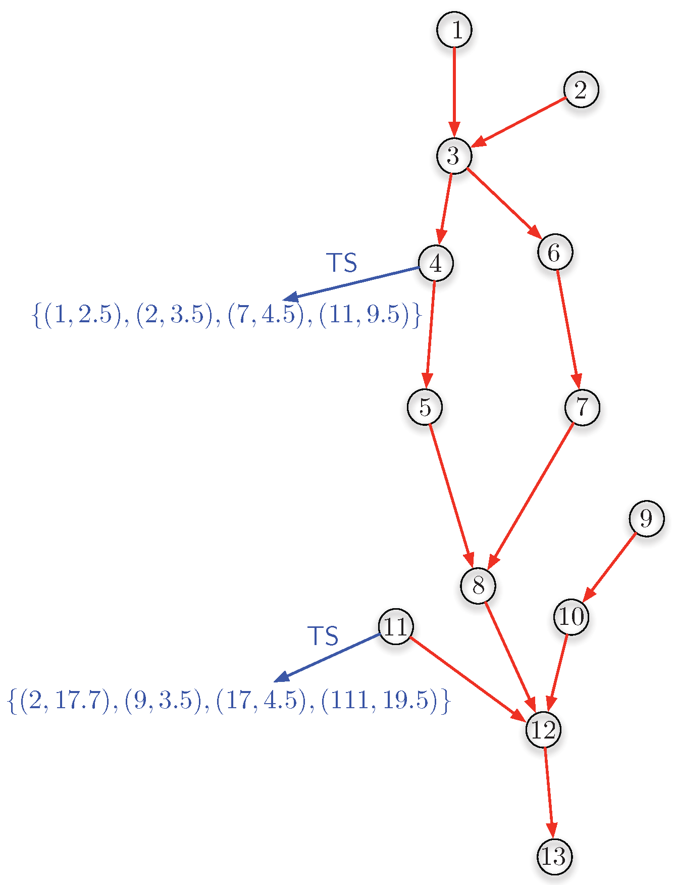
In this paper we assume that river segments are modelled as nodes in a graph and the edge relation expresses that water flows from one river segment to a next. Therefore, in the context of river systems, we denote the edge as the relation. Figure 1 shows our abstract graph representation of a transportation network. In this figure, river segments are represented by nodes, and an edge between two nodes A and B indicates that the water flows in the direction of the edge. In the figure, the node set models 13 river segments and the relation is represented by the red arrows. The figure shows two sensor nodes with their time series in blue, denoted . Time series are composed of pairs of the form (value, instant).

Figure 1.
A transportation network shown as a directed graph in which the relation is depicted by the red arrows. In this example, nodes 4 and 11 are sensors and they are shown together with the time series attached to them (shown by the blue arrows).
3.2. Temporal Graphs
Next, we give some basic definitions about temporal graphs that we use throughout the paper. These definitions, unless noted, are taken from [5]. In what follows, we work with graphs where nodes, relationships, and properties are timestamped with a temporal validity interval. We also assume that graphs are heterogeneous, meaning that relationships may be of different kinds.
Definition 1
(Temporal property graph (from [5])). A temporal property graph is a structure where G is the name of the graph, E is a set of edges, and and are disjoint sets of nodes, called object nodes, attribute nodes, and value nodes, respectively. Object and attribute nodes, as well as edges, are associated with a tuple . The represents the content of the node (or the type of the edge), and the the time period(s) when the node is (or was) valid. Analogously, value nodes are associated with a pair. For any node n, the elements in its associated pair are denoted as , , and . As usual in temporal databases, a special value tells that the node is valid at the current time. All nodes also have an (non-temporal) identifier denoted .
In Definition 1, object nodes are typically used to represent entities (e.g., ), while edges represent relationships between object nodes (e.g., , ). Attribute nodes are use to describe the properties of an entity (e.g., ). Finally, value nodes represent the value of an attribute (e.g., Mary).
Nodes and edges in G satisfy a collection of temporal constraints that we intuitively comment on next. All nodes in the graph must have a different identifier (). Also, all nodes with the same value associated with the same attribute node must be coalesced into one. Thus, the interval becomes a temporal element (that is, a set of intervals) which includes all periods where the node has such value. The same applies to edges: all edges with the same name (that is, representing the same relationship type) between the same pair of nodes, must be coalesced into a single one. Nodes must be connected as follows: (a) an object node can only be connected to an attribute node or to another object node; (b) attribute nodes can only be connected to non-attribute nodes; and (c) value nodes can only be connected to attribute nodes. The cardinalities of these connections are such that attribute nodes must be connected by only one edge to an object node, and value nodes must only be connected to one attribute node with one edge. Finally, intervals must satisfy the following: (a) the interval of an attribute (value) node must be included in the interval of its associated object (attribute) node; (b) the intervals associated with a value node must be disjoint; (c) the intervals of two edges between the same pair of nodes must be disjoint.
Following this model, different notions of temporal paths are defined. These were intuitively introduced in Section 1, so we do not repeat them here. In the following sections, we show how we extend them to support transportation networks.
The model described above comes with a high-level query language denoted T-GQL. The language has a slight SQL flavor, although it is also based on Cypher. One of the features that make Cypher a popular query language is the possibility of adding libraries of functions that extend its functionality. Therefore, T-GQL extends Cypher with a collection of functions that allow handling the different kinds of temporal paths introduced above. For example, the function computes the Continuous Paths in a transportation network (see the example below) is included in this library, and immediately available to be used in a Cypher query. The same for example with , which computes the Pairwise Continuous Paths. The use of these functions is explained in detail in Section 7. Finally, T-GQL queries are translated into Cypher, hiding all the underlying structures that allow handling a temporal graph. Details of this implementation can be found in [5]. As an example to give the intuition of the language, consider the query “Paths where temperature was High simultaneously, between ‘2022-03-10 05:00’ and ‘2022-03-10 16:00’, starting from the sensor located at segment 3. The number of sensors in the returned path must be between 3 and 5.” In this query we assume that nodes contain, the property, which is a categorical time series with possible values High, Medium and Low. Variable categorization is explained in Section 7.2. The T-GQL expression for this query is:
1  SELECT paths
2  MATCH (s1:Sensor), (s2:Sensor),
3  paths = TNCP((s1)-[:flowsTo∗3..5]-> (s2),
4          ‘2022-03-10 05:00’, ‘2022-03-10 16:00’,
5          ‘Temperature’,’=’, ‘High’)
6  WHERE  s1.id = 3;
As mentioned, the T-GQL syntax is built as a combination of SQL and Cypher. In what follows we assume GIS readers are familiar with SQL. For the Cypher part, we can see the MATCH statement, which basically defines a pattern that the engine looks for in the graph. Thus, a Cypher query is also a graph, and the answer to the query is composed of all the subgraphs that Cypher finds in the graph database. In the query above, we define two variables s1 and s2 for the initial and final sensors in a path. In the query, paths is a variable which, because of the “=” sign, represents a path. The expression represents the pattern to be matched. It indicates all the paths between two nodes, with a length between 3 and 5, along the relationship . Also, in the query above, the function computes the Continuous Paths indicated by the pattern, within the time close-open window [‘2022-03-10 05:00’, ‘2022-03-10 16:00’), such that the value for the is High, starting at node 3 (). The function parameters ‘’ and indicate, respectively, the variable and the value for the variable to use in the definition of the CP. The parameter ‘=’ in the function indicates that we require the equality as the condition of the path. The following example shows that this is not the only option.
As another example, the following query computes the Pairwise Continuous Paths, where the value of electrical conductivity was greater than or equal to Medium between ‘2022-03-10 05:00’ and ‘2022-03-10 16:00’, starting from the sensor in Segment 3.
The T-GQL expression for the query above is given next.
1 SELECT paths, interval
2 MATCH (s1:Sensor), (s2:Sensor),
3 paths = TNPCP((s1) - [:flowsTo∗] -> (s2),
4         ’2022-03-10 05:00’, ’2022-03-10 16:00’,
5         ’Temperature’,’up’, ’Medium’)
6 WHERE s1.id = 3;
In this query, the function computes the Pairwise Continuous Paths using the Cypher pattern , which finds all paths of any length between two nodes, within the specified interval also starting from node 3. The function parameters ‘’ and ‘Medium’ indicate, respectively, the variable and the value for the variable to use in the definition of the path. The parameter ‘’ indicates that we do not just require the equality as the condition of the path, but we are also looking for paths where temperature is constantly increasing.
4. Temporal Graphs for Transportation Networks
The model in Definition 1 must be modified to capture the characteristics of transportation networks. For example, we must distinguish object nodes that hold a sensor from the ones which do not. We call the former segment nodes. A property with a specific value Sensor, together with a list of intervals, indicates the periods of time where a segment has a working sensor on it. This allows, for example, representing the addition of a new sensor, the presence of a sensor that no longer works, or the removal of a sensor. Properties that do not change across time are represented as usual in property graphs. We remark that we work with categorical variables in the time series attached to the nodes in the graph. The process to transform continuous values (provided by the sensors) to categorical variables is explained in Section 7.2. Also, we assume that there is at most one sensor per segment, which can measure different variables.
Definition 2
(Transportation network temporal graph). A Transportation Network Temporal Graph (TNGraph) is a structure where G is the name of the graph, E a set of edges, and , , and sets of nodes, denoted segment, attribute, and value nodes, respectively. Nodes are associated with a tuple , but in segment nodes this tuple exists only if the segment contains (or ever contained) a sensor. In this case, = Sensor, and represents the periods when a sensor worked. They may also have properties that do not change over the time (called static properties). An attribute node represents a variable measured by the sensors, its property is the name of such variable, and is its lifespan. A value node is associated with an attribute node, and its property contains the (categorical) values registered by the sensors, and represents the period when the measure was valid. The property of the edges between segment nodes represents the flow between two segments, and is the validity period of the edge. All nodes have a static identifier denoted .
The constraints mentioned in Section 3.2, also hold for the model in Definition 2. However, they must be modified and extended to represent the transportation network characteristics. For example, an attribute node can be connected to a segment node only if that segment once had a sensor. In addition to the above, a constraint is added to express that the flow between two segments is in only one direction at any given time.
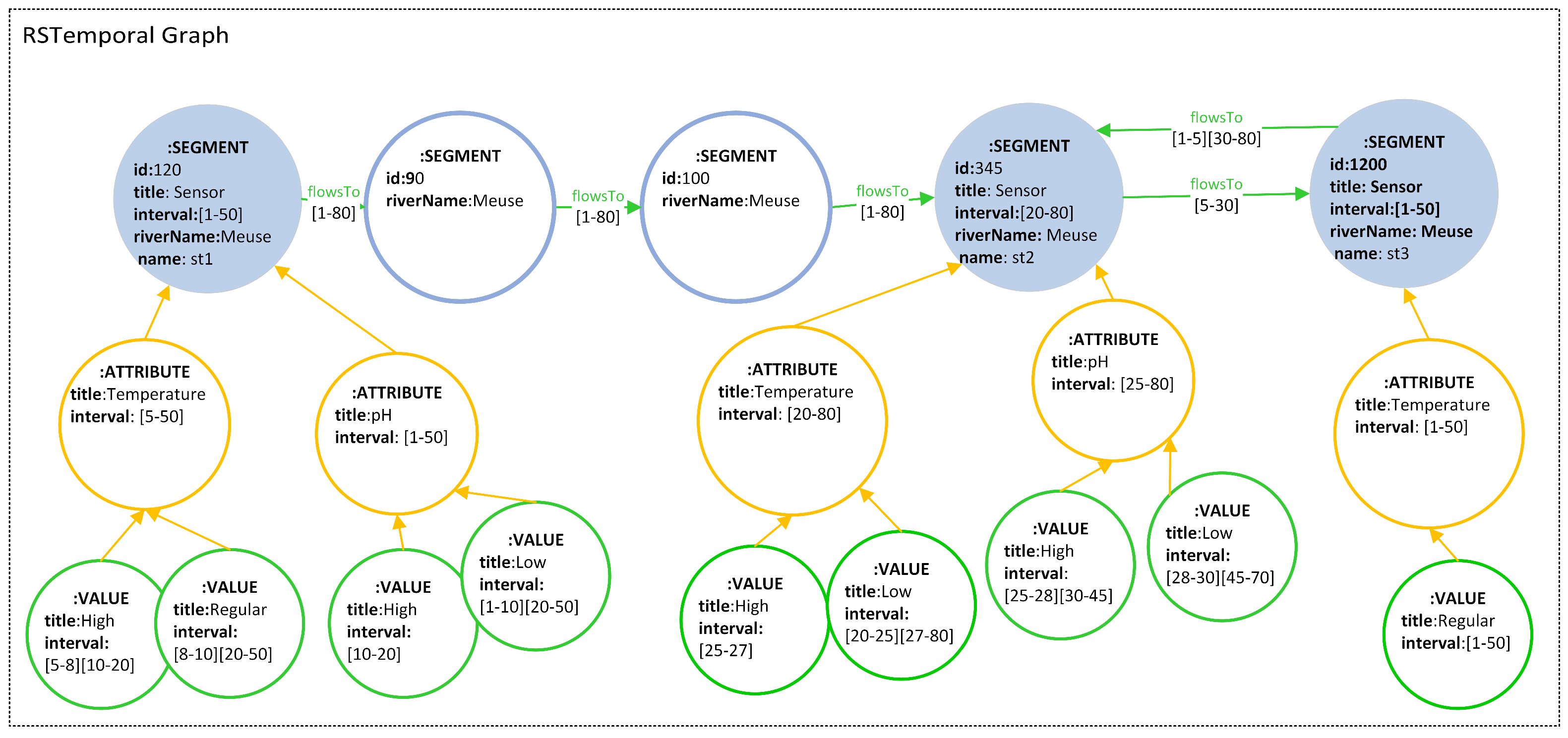
As an example, consider a river system (just as an illustration, we used the river Meuse) in the Flanders river system. Figure 2 illustrates the model of a portion of a river based on Definition 2. Three out of the five segments considered have a sensor on them. Thus, the TNGraph has five segment nodes, one for each segment, and three of them (the ones with = 120, = 345, and = 1200) have the property title = Sensor. All segment nodes have a static property , which contains the of the river, and name, which contains the name of the sensor station. Segment with = 345 had a sensor between times 20 and 80 and measured two variables: and . Therefore, there are two attribute nodes connected to it, one for each variable. Please note that the time interval of the attribute nodes satisfies the temporal constraints, for example, the interval is included in the interval of the segment node. In this case, the interval of the segment node is [20-80), the interval for the attribute node is [25-80) and the interval for the node is [20-80). We remark that the interval brackets of Figure 1 express the list in which they are stored, but they are interpreted as close-open intervals. There are two value nodes for the attribute node, and its property expresses that between instants 20 and 25 the temperature was Low, between instants 25 and 27 it went up to High, and between instants 27 and 80 it went down to Low again.
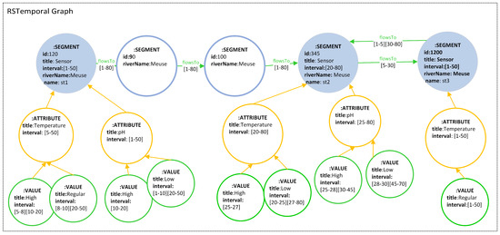
Figure 2.
A temporal graph for a river network with sensors measuring Temperature and pH.
This example shows that the model allows representing the change of the direction of the flow (in this case, between nodes 1200 and 345), and also situations where we have a hybrid representation of nodes with or without sensors. Nevertheless, in our use case we do not require such features, since in the portion of the river we will consider, water only flows in one direction.
The model introduced and discussed in this section is powerful enough to express a wide range of temporal queries, typical in the field of temporal databases. However, in the remainder, we will focus on path queries, that is, queries that compute different kinds of paths in a graph. Our temporal graph model supporting time series, allows the definition of many different kinds of temporal paths, which are studied in the next section. After defining these paths, we explain how we can compute them and how this mechanism can be applied to a real-world case such as a river system in the region of Flanders in Belgium.
5. Paths in Transportation Networks
There are many queries of interest for hydrologists that can be answered using the model described in Definition 2. For example: “Starting from a segment, obtain all the paths and their corresponding time intervals such that the value of the electrical conductivity along the path has been simultaneously High for all nodes in the path during a certain interval I”, or “Starting from a segment and given a time interval I, obtain the longest time period within I such that the electric conductivity value in those segments has been simultaneously High for a consecutive sequence of river segments.” These queries can be captured by extending the different notions of temporal paths. In particular, the queries above are captured by CPs extended to support time-series functions. In this section, we study and present these extensions, based on the model of Definition 2. We call these paths Transportation Network Continuous Path (TNCP), Transportation Network Pairwise Continuous Path (TNPCP), and Transportation Network Consecutive Path (TNP). We generalize this concept defining a new class of path denoted Transportation Network Flow Path.
5.1. Transportation Networks Continuous Path
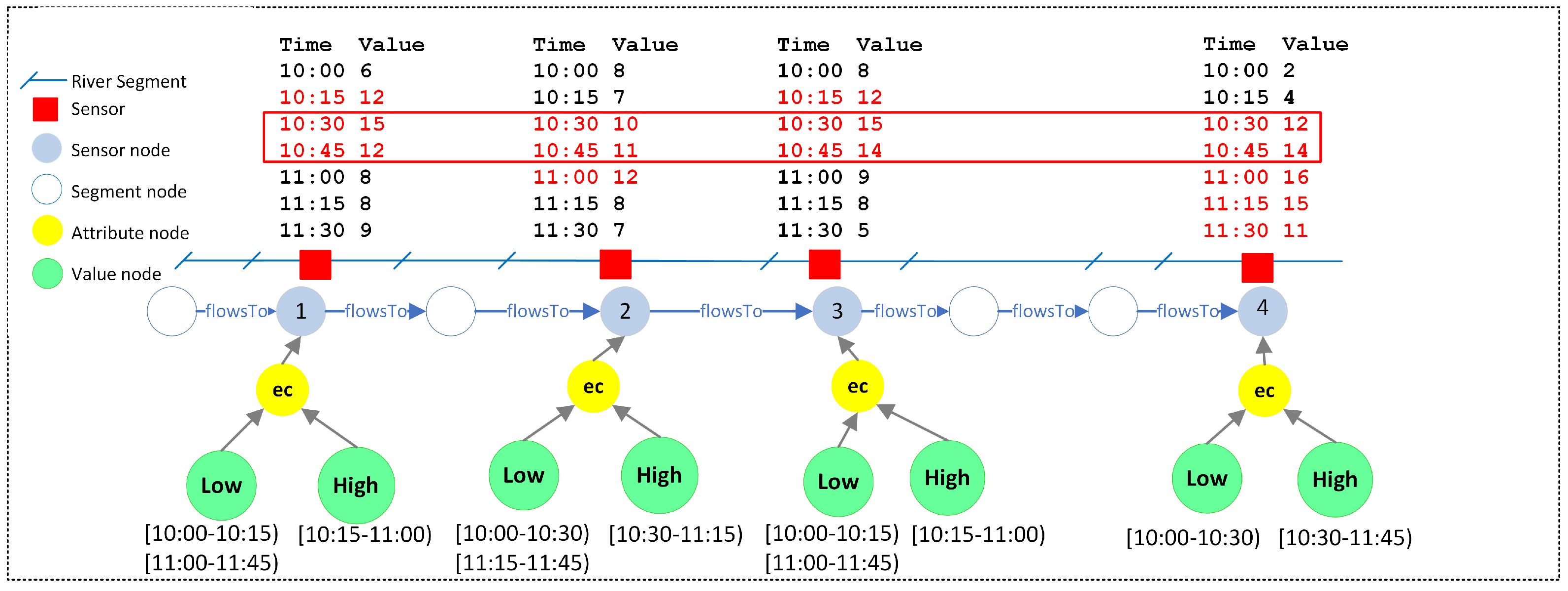
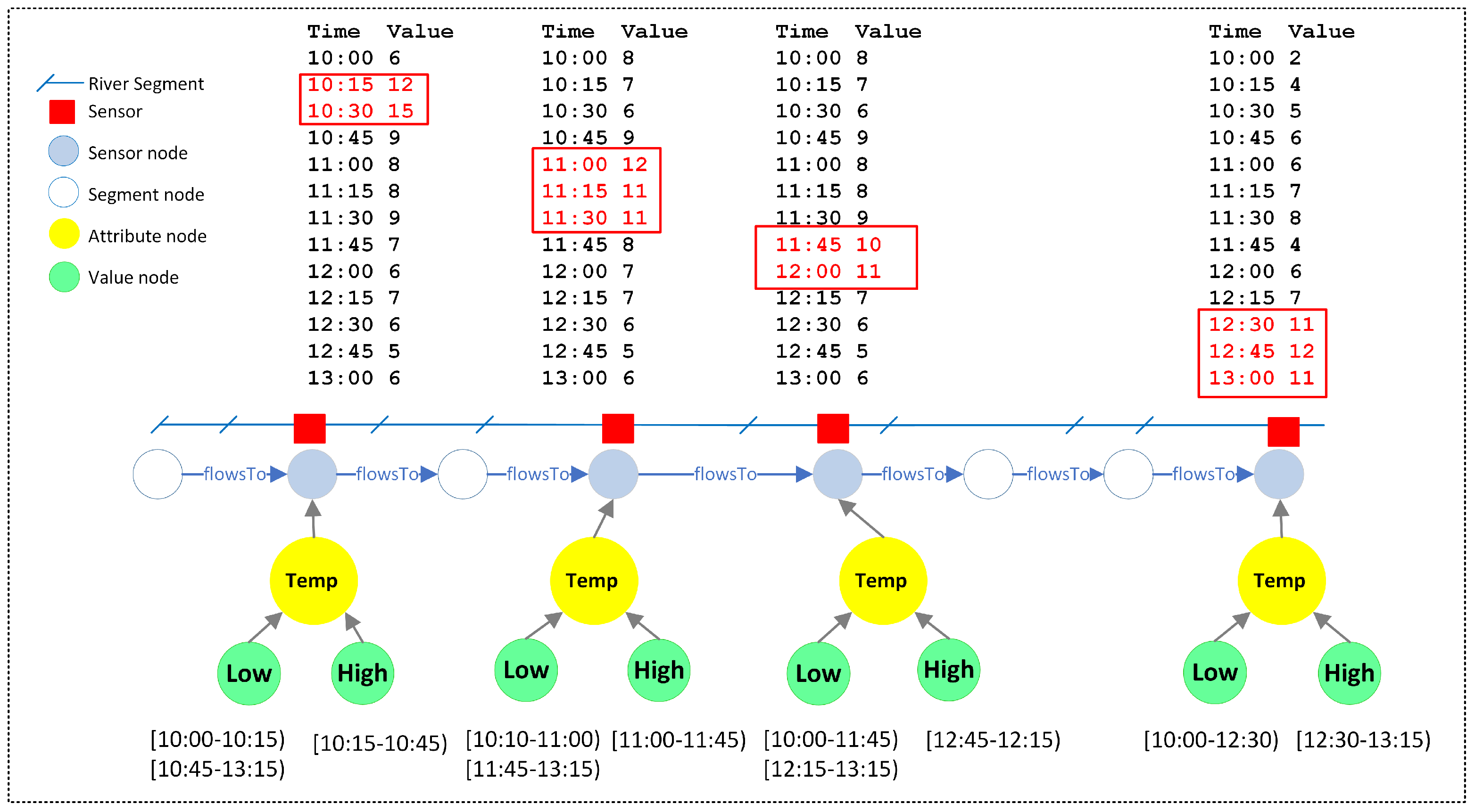
The queries above capture events that occurred simultaneously at different places. The idea is to find all the consecutive sensors that registered an event at the same time and return those sensors, the segments in-between, and the time intervals when these events occurred. The original Continuous Path notion introduced in [5] only accounts for the connections between nodes in a temporal graph, and must be modified to compute a path restricted to a certain value of a variable measured by the sensors. This is illustrated in Figure 3, which depicts a portion of a river represented as a temporal graph (in the lower part), and electric conductivity (in the figure ) measures registered by sensors every fifteen minutes (in the upper part). Sensor nodes in the river are denoted by a filled red square. Values categorized as High for the variable ec are denoted in red over the registered measurement. We can see the time interval [10:30–11:00) where the value is High for all the sensors, and this is framed in the figure. The lower part of the figure shows the corresponding TNGraph, where we can also see nodes with no sensor. Based on the above, we can now define the notion of Transportation Network Continuous Path.
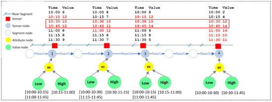
Figure 3.
Transportation Network Continuous Path for .
In the definitions next, the following notation is used: (a) an edge e between two nodes and is denoted ; (b) an attribute node is denoted where o is the object node connected to a; (c) a value node is denoted where a is the attribute node connected to v; is the value of the value node v associated with the attribute node a associated with the object node o.
Definition 3
(TN Continuous Path). Let G be a TNGraph, and a temporal variable that can take n possible values from a domain , during a certain time interval. A TN Continuous Path (TNCP) with respect to with interval T from node to node , traversing edges of type R, is a structure , where S is a sequence of k nodes , such that
- ;
- ; and
- T is an interval such that for all i there exists , and such that
- -
- ;
- -
- ;
- -
- ; and
- -
- .
Between a pair of sensor nodes, a path can exist, where is a segment node with no sensor.
We note that in the definition above, when we consider a river system, R becomes the relationship indicating the direction of the water flow.
In Definition 3, the relation between every pair of consecutive intervals , , corresponding, respectively, to sensors and , where = and =, is expressed by:
( ) ∨ ( by ) ∨ ( ) ∨ ( ), where we use relations from Allen’s interval calculus [28]. Here, and are the inverse of each other, indicating that two time intervals overlap. Analogously, and are the inverse of each other, and mean that one interval is completely included in the other one.
On top of the above, there is an interval T included in every .
Example 1.
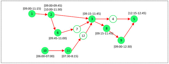
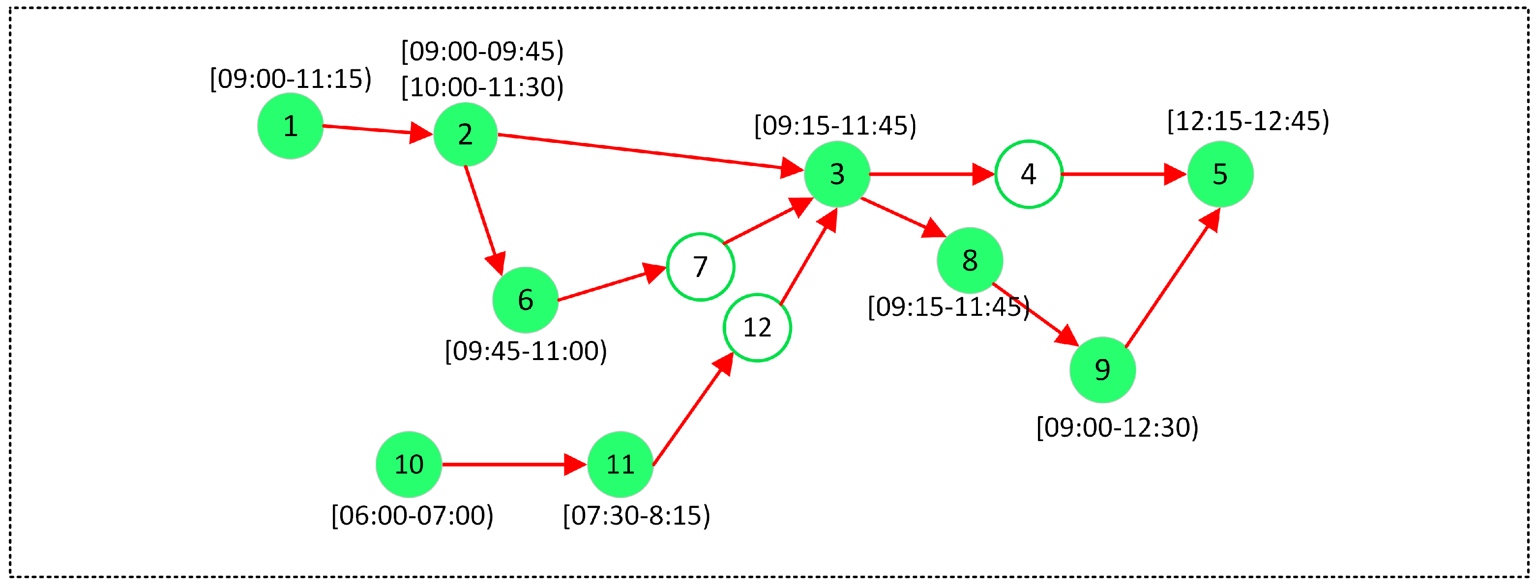
Figure 4 shows a simplified representation of an TNGraph where we only show the intervals when the value High of the variable occurred. Filled nodes represent segments with a sensor and non-filled ones represent nodes without sensors (in this case, nodes 4, 7 and 12). Consider a query asking for all the continuous paths between nodes 1 and 9, with a High value of the temperature between 09:00 and 12:00, restricted to a minimum of 5 sensor nodes and a maximum of 7. For the graph in the figure, the query returns three TN continuous paths:

Figure 4.
Simplified TNGraph where nodes with attribute have associated intervals. Every node represents a river segment and sensor nodes are filled in blue.
- , [09:15–09:45]]
- , [10:00–11:15]]
- , [10:00–11:00]].
After obtaining the three paths above, we could select the one with the maximum number of sensor nodes (in this case, as it has 6 sensor nodes while the other ones have 5). We could also compute the path with the largest interval (in this case, , with a duration of 75 min).
5.2. Transportation Networks Pairwise Continuous Path
Requiring a path to be valid throughout a time interval is a strong condition for a graph query. In many cases, querying temporal graphs requires a weaker notion of temporal path. The user may be interested in a transitive relationship such that there is an intersection in the interval of two consecutive sensor nodes. For example, consider the query: “Starting from a segment obtain all the paths where for every segment and the one immediately following it, the temperature was simultaneously High during an interval, i.e., all the paths formed by the segments of the river such that ”. This query requires that the function has a value High not continuously throughout a path, but only in a pairwise fashion between consecutive segments containing a sensor.
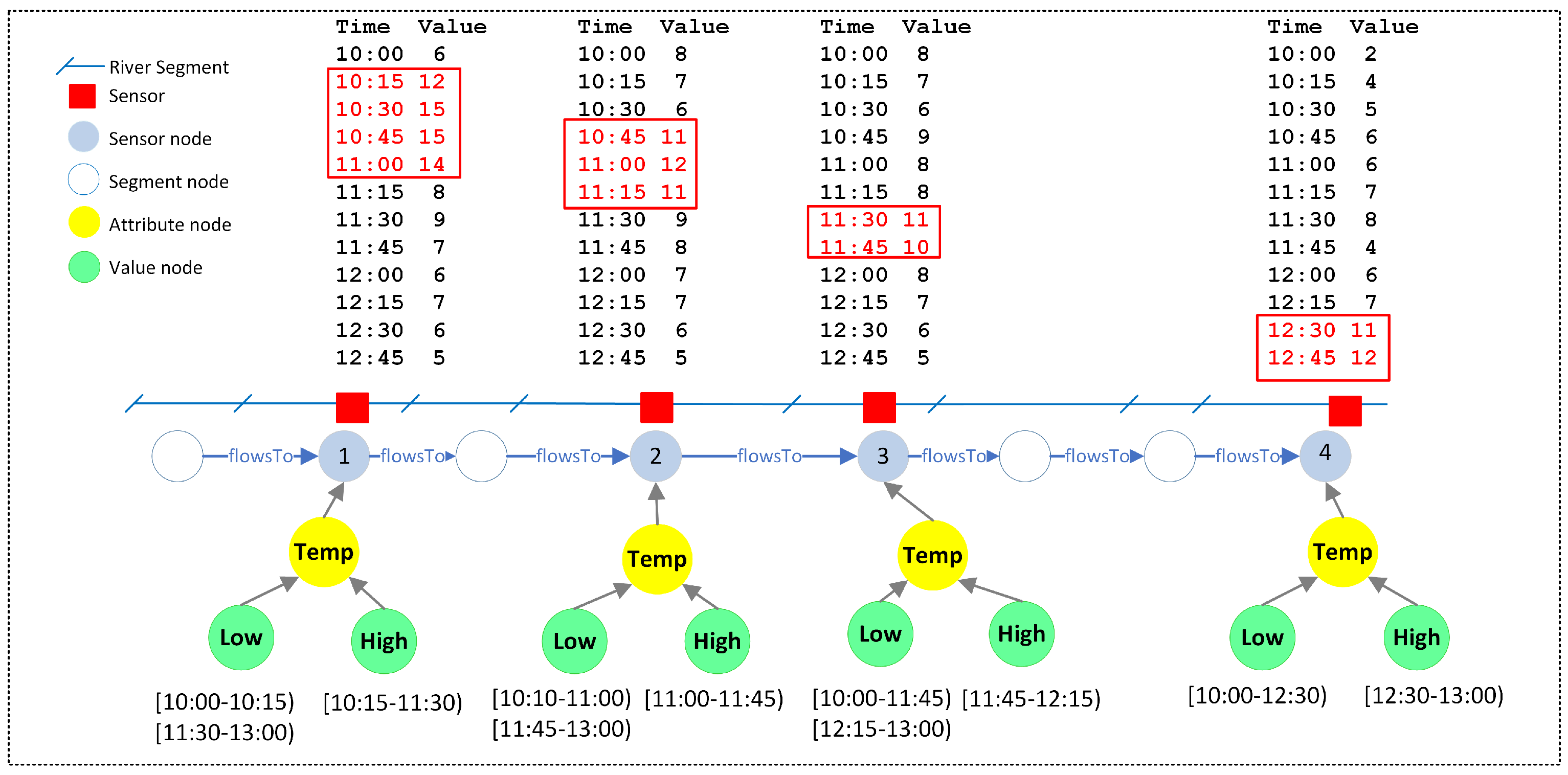
To be more precise, consider the case of a river network like the one in Figure 5. There is no TNCP with = High that involves the four sensors (for clarity reasons, is abbreviated as in this figure and the following ones). However, the value of of the first pair was simultaneously High during the interval [10:30–11:00); it was also High for the next two segments during [11:15–11:45) and it was High as well for the last two during [11:30–12:00). That means, although there is no RCP between the four sensors, there is a consecutive chain of pairwise temporal relationships between them. This is formalized by the notion of TN pairwise continuous path (TNPCP).
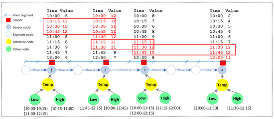
Figure 5.
Transportation Network Pairwise Continuous Path of .
Definition 4
(TN Pairwise Continuous Path). Let G be a TNGraph, and a temporal variable that can take n possible values from a domain , during a certain time interval. An TN pairwise continuous path (TNCP) with respect to from node to node , through a relationship R, is a structure , where S is a sequence of k nodes such that
- ;
- ; and
- T is a list of intervals such that there exists such that
- -
- ;
- -
- ;
- -
- and
- -
- is a list of intervals such that .
Intuitively, the condition above means that whenever there are two value nodes with the same value corresponding to the same attribute node in two consecutive sensor nodes, we take the intersection of their corresponding time intervals. The TNPCP will be formed by a sequence of sensor nodes and the intersections of their time intervals.
Between every pair ( of sensor nodes in the path, a path of the form can exist, where is a segment node with no sensor.
Example 2.
Consider a query over the graph of Figure 4 asking for all the pairwise continuous paths between nodes 2 and 5, with a High value of the temperature between 09:00 and 12:45, restricted to a minimum of 4 sensor nodes and a maximum of 7. The query returns three TN pairwise continuous paths:
- , {[09:15–9:45][09:15–11:45][09:15–11:45] [12:15–12:30]}]
- , {[10:00–11:30][09:15–11:45][09:15–11:45] [12:15–12:30]}]
- , {[10:00–11:00][09:45–11:00],[09:15–11:45] [09:15–11:45][12:15–12:30]}]
We can see that, although there is no continuous path between nodes 2 and 5, there is a pairwise continuous path between those nodes.
5.3. Transportation Networks Consecutive Path
Due to the distance between sensors, sometimes a network analyst may look for events occurring in a way such that the period of time in which a sensor detects that event does not overlap with the time period during which the next sensor on a path registers it. For example, in a river where there is a long distance between sensors, if a substance that modifies the electrical conductivity, temperature, or any other parameter, is spilled into the water close to a measuring station, it is possible that the effect is not registered at the following one in downstream direction. As an example, the upper part of Figure 6, the first sensor on the left registered a High temperature value from 10:15 through 10:45. The next sensor detected a High value of temperature from 11:00 through 11:45. The third sensor registered a High value between 11:45 and 12:15. That means, there is no overlap between the time intervals or, in other words, the interval of the next period starts after the previous one has finished. This example is captured by the notion of consecutive path. That is, a path composed of sensor nodes such that for every pair of consecutive sensors the value of a temporal variable is the same during two consecutive non-overlapping intervals. We denote this path a Transportation Network Consecutive Path for .

Figure 6.
River network Consecutive Path with .
Definition 5
(TN Consecutive Path). Let G be a TNGraph, and a temporal variable that can take n possible values from a domain , during a certain time interval. A TN consecutive path (TNP) with respect to , traversing a relationship R in G, is a structure , where
- S is a sequence of pairs where is the i-th sensor node in S, for such that there exists
- -
- such that
- -
- ;
- -
- ;
- -
- and T is a list of intervals .
- For every pair , , it holds that
- -
- .
Between every pair of sensor nodes , , a path of the form can exist, where is a segment node with no sensor.
Example 3.
A query over the TNGraph of Figure 4 asking for all the consecutive paths between nodes 10 and 5, with a high value of temperature, between 06:00 and 13:00, restricted to a minimum of 4 sensor nodes and a maximum 5, one consecutive path: , {[06:00–07:00][07:30–08:15][09:15–11:45][12:15–12:45]}].
Observe that the interval for every sensor node of the path does not overlap with the next one.
5.4. Transportation Networks Flow Paths
The paths defined above refer to one single kind of path capturing the characteristics of the flow in a transportation network using the value of categorical variables. Sometimes, considering these kinds of paths separately is not enough to capture the characteristics of the flow. For example, in [29] the authors model the traffic flow patterns produced by moving objects using a semi-Markov chain over a graph to model delays at each transition. This scenario may also occur in river networks: an event (e.g., the presence of a pollutant) detected by one sensor may still be happening when it is detected by the next sensor. Pairwise Continuous Paths (Definition 4) require that intervals between every consecutive pair of segments overlap along the whole path, while Consecutive Paths (Definition 5) capture non-overlapping consecutive temporal paths. The example above actually requires a mix of these path, since the time at which an event is first detected on one sensor must be earlier than the first time the same event is registered on the next segment. Figure 7 illustrates this situation. Here, a High value of Temperature is detected in one sensor earlier than the fist time it is detected in the next consecutive one. Here, the measurement of the first pair of sensors overlap, but the measurements of the second and third pairs do not. We call these kinds of paths Flow Paths.
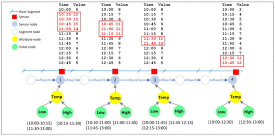
Figure 7.
River Network Flow Path for .
Definition 6.
Let G be a TNGraph, and a temporal variable that can take n possible values from a domain , during a certain time interval. A TN Flow Path (TNFP) with respect to traversing edges of type R in G, is a structure , where
- S is is a sequence of pairs
- is the i-th sensor node in S, for , and there exists
- -
- such that
- -
- ;
- -
- ;
- -
- and
- -
- .
- For every pair , it holds that
- -
Between a pair of sensor nodes , a path , …, can exist, where is a segment node with no sensor.
Example 4.
Consider Figure 4. A query that asks for all the Flow paths starting at node 2 where the temperature was High between 09:00 and 13:00, restricted to a minimum of 3 sensors returns only one TN Flow path, involving sensor nodes 2, 3, and 5, as follows: , {[09:00–9:45][09:15–11:45][12:15–12:45]}]
Observe that the intervals for segments 2 and 3 overlap but the ones for segment 3 and 5 do not.
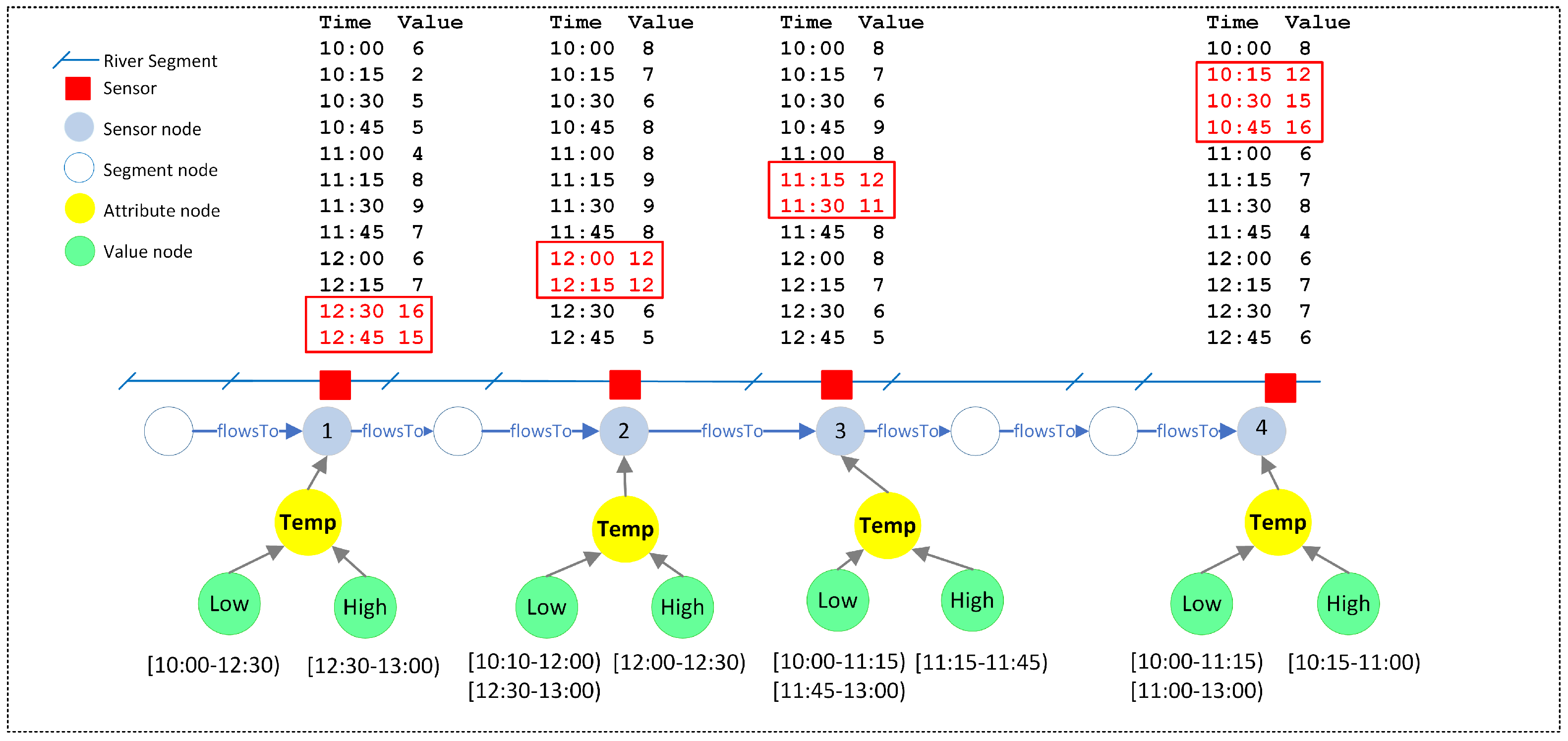
An interesting situation occurs when the impact of an event propagates in the direction opposite to the flow. A typical example is a road network, where the effect of a traffic jam propagates backwards (in the opposite direction of the traffic movement), reducing the speed before the point where the traffic was interrupted. The same effect can be detected in rivers in locations close to the sea, when the tide moves towards the shore. This is captured by the Flow Path in Definition 6, but where propagation operates backwards. In this case, from the starting node, where the event is detected, we follow the path using the incoming edges instead of the outgoing ones. Thus, there are two variations of the TNFP: forward and backwards. We call the latter a TN Backwards Flow Path (TNBFP), to distinguish the case in which the value of a variable propagates against the flow from the case when the variable propagates downstream. As a convention, when a TNFP is “forward” we just call it TNFP. In Figure 8, we can see that the High values of water temperature are produced earlier in the nodes closer to the sea, that is, the High temperatures arrive later to the sensors that are farther from the sea. For example, temperature was High Node 4 at 10:15, but this effect only reached Node 1 at 12:30.
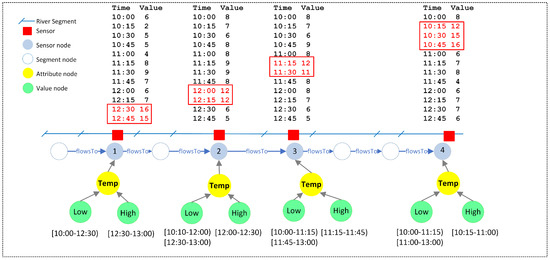
Figure 8.
River Network Backwards Flow Path for .
Example 5.
Consider Figure 4. A query that asks for all the Backwards Flow Paths starting at node 3 where the temperature was High between 09:00 and 13:00, restricted to a minimum of 2 sensors returns two TN Flow Backwards paths, involving sensor nodes 3, 7, 6 and 2, as follows:
- , {[09:15–11:45][10:00–11:30]}]
- , {[09:15–11:45][09:45–11:00][10:00–11:30]}].
5.5. Generalizing Temporal Paths
Definitions 3–6 are based on the value of a categorical variable. This is in fact rather limiting, since it leaves out a number of interesting situations. For example, a TNCP can be defined as a path where the value of an ordered categorical variable continuously increases (or decreases) during a certain interval rather than remaining the same, as we considered so far. For example, it may be interesting to check when the water temperature continuously decreases from Sensor 1 to Sensor 3 in the interval . Thus, in this case we are looking for a “decreasing continuous path”.
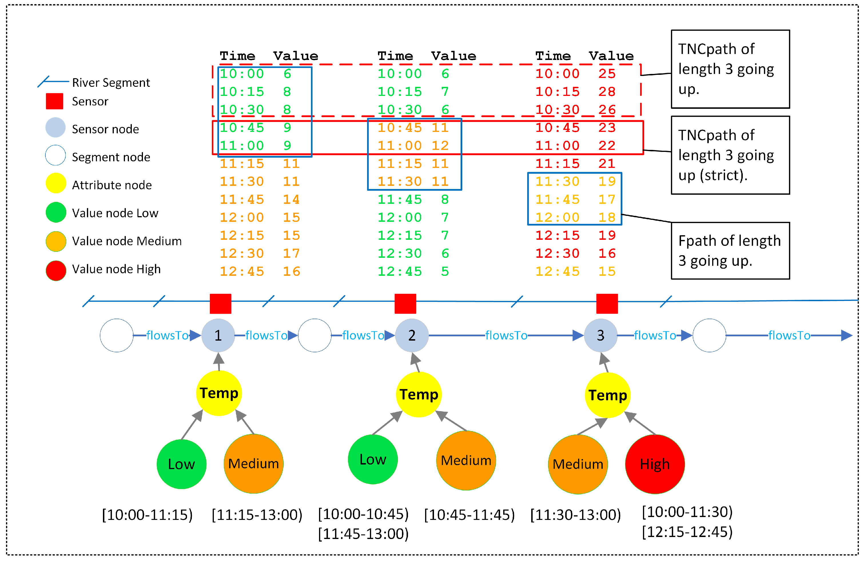
As an example, consider Figure 9. Here, to make the figure clearer, we used different colors for the values of the Temperature variable, which is categorized as: Low (green), Medium (orange) or High (red), using the thresholds 10 and 20. For example, Node 1 presented a Low value from 10:00 to 11:15 and Medium from 11:15 to 13:00. There is no High value for this node. If we consider paths of length 3 and the values going strictly up, we will find one TNCP from 10:45 to 11:15. During that time, station 1 has a Low value, Station 2 has a Medium value and Station 3 has a High value. In that Figure, this path is denoted with a red solid line box over those times. We may also ask that a value in a path remains the same or higher than in the previous node. This is the case of the path indicated by the red dashed line.
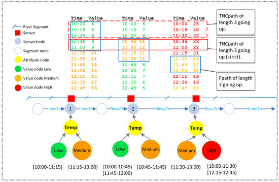
Figure 9.
River Network Continuous Path of going up.
We can see that this generalization adds expressive power to the language, particularly considering real-world applications, where asking for strictly equal values of the variables, may leave out interesting practical cases. We remark that we preferred to keep the formal definitions simpler, without losing generality, and this is the reason why we did not include the general case in the definitions above.
6. Path Computation and Query Generation
In this section, we show how the paths defined in the previous section are computed, and how a T-GQL query is processed extending Neo4j with a collection of procedures stored in the database’s Plugins folder. A procedure is created for each one of the definitions in Section 5. The T-GQL is translated into a Cypher query, which is then processed by the Neo4j engine, extended with the libraries we developed. We first present the algorithms that compute the TN paths (to avoid redundancy we show the algorithm computing Flow Paths) and then we show how all the machinery is applied to process a T-GQL query.
6.1. Computing the TN Temporal Paths
Algorithm 1 describes the computation of the (forward and backward) Flow Paths in a graph representing a TN (Definition 6). The algorithm receives a temporal graph the source and (optionally) destination nodes (s and d, respectively), a variable X, an operator , a value v, a time interval , a direction (to handle forward and backward paths) and a value that limits the time gaps between sensors. It returns the set of Flow Paths that satisfy the query. The algorithms that compute the other kinds of paths proceed analogously, and we omit them to avoid redundancy and for the sake of brevity. We remark that Algorithm 1 addresses the general case described in Section 5.5, this is why the operator is required as input.
Algorithm 1 builds a transformed graph , whose nodes contain either the interval when the value of X v was valid (if they are sensor nodes) or the interval of the previous sensor in the temporal graph, and the edges indicate the nodes reachable from that position. The nodes n in have seven attributes: a reference to the node in the original graph (), a flag telling whether the node is a sensor or a non-sensor one (), a time interval when the value of X v was valid () along with the value (), the number of sensors in the path (), the total number of nodes of a path so far (), and a reference to the previous node in , (), that allows rebuilding the paths after running the algorithm. In short, is a tuple .
| Algorithm 1 : Computes the Flow Paths |
Input: A graph G, a source node s, a destination node d (optional), a variable X, the maximum number of sensors in the path , a query interval , an operator , a starting value v, the direction and a period of time. Output: A set with the solutions.
|
Algorithm 2 is called by Algorithm 1, and contains the function that retrieves the pair (interval, value) according to the operation in the FPath query. It receives an attribute node that holds the value nodes for the variable X, the query interval , the interval of the previous sensor I, the operator , a value v and a period . For each value node connected to , if X is true, a function returns the first interval whose start time is greater than the start time of the previous interval I and within the indicated period . Finally, the function returns the closest interval and its corresponding value .
| Algorithm 2 : Obtains the interval of a sensor node according to an operator |
Input: A graph G, an attribute node a, a query interval , a previous interval I, an operator , a starting value v, a period . Output: An interval and its value .
|
In the next section we explain these algorithms through a concrete example, taken from our use case.
6.2. Processing T-GQL Queries
T-GQL queries are parsed and translated into a Cypher query that is run on a Neo4j database. As mentioned, the procedures that implement the path-finding functions are stored as Neo4j plugins. As mentioned previously, although the user perceives a temporal graph representing a transportation network as a graph like the ones in Figures 16 and 18 (explained later), behind the scenes, the underlying graph has the form indicated in Figure 2, where we can see object, attribute and value nodes. Therefore, the user asks the queries over the former kind of graph, that is, the one that intuitively is closer to how she perceives the network, but the query is translated into the structures of the latter. The next example explains the above.
Consider the following query over the graph in Figure 9:
Get the Flow Paths of length at most 3, such that the value of raises from the value Low, starting from Node 1, occurring between ’2022-03-09 09:30’ and ’2022-03-09 13:00’ and such that the delay between the first time an event is registered at one sensor and the time when it is detected at the next one is less than one day.
The query in T-GQL is expressed as follows (the “up” parameter represents the condition asking for increasing values of the variable, the delay is expressed as ‘P1D’):
1 SELECT p.path, p.intervals
2 MATCH (p1:Sensor), (p2:Sensor),
3     p=fPath((p1) - [f:flowsTo∗3] -> (p2),
4     ’2022-03-09 09:30’,’2022-03-09 13:00’,’Temperature’,
5     ’up’,’Low’,’P1D’)
6 WHERE p1.Name = ’1’
The T-GQL engine translates the query into the following Cypher query, expressed in terms of the underlying temporal graph structure (we omit the details of this translation since this is beyond the scope of the paper):
1 MATCH (p1:Segment {title: ’Sensor’}),
2 (p2:Segment {title: ’Sensor’})
3 WHERE p1.name = ’1’
4 CALL consecutive.sensorFlowing(p1,p2,3,3,
5         {edgesLabel:’flowsTo’,delta:’P1D’,
6          attribute:’Temperature’,category:’Low’,
7          between:’2022-03-09 09:30 - 2022-03-09 13:00’,
8 operator:’up’,direction:’outgoing’})
9 YIELD path as internal_p1, intervals as internal_i1
10 WITH {path: internal_p1, intervals: internal_i1} as p
11 RETURN p.path, p.intervals
It can be seen that this Cypher query calls the consecutive.SensorFlowing procedure (implemented by Algorithm 1) which is executed on Neo4j and the result is returned to T-GQL. We also remark that the complexity of the query that is actually executed is hidden from the final user, who must only write a short and intuitive query in an SQL-like query language.
We next explain how the procedure consecutive.SensorFlowing works using the T-GQL query above applied to the graph in the lower part of Figure 9.
In the initialization part, the source node s is Node 1, and we can see that there is no destination node in the query. The variable X is , the number of sensors is 3, the query interval is [2022-03-09 09:30–2022-03-09 13:00], the operator is “up”, the direction is “outgoing” and the period is “P1D” (meaning one day).
First, in Line 2, the function checks if there is a node, , connected to s where . In this case there is one, thus, in Line 4, the function (see Algorithm 2) is called to obtain the first interval. This function receives , [2022-03-09 09:30–2022-03-09 13:00], [2022-03-09 09:30–2022-03-09 13:00] (the previous interval, in this case the same as ), “”, and “P1D”. The function (Line 3) is called to obtain all the value nodes connected to a in the original graph. The first value node obtained is the one with value , thus we make . Given that is “up”, the switch command chooses the “up” option (Line 10). After this, since and is null at this time, the function picks the list of intervals in (here, only [[10:00–11:15]]), and returns the interval whose start time is greater than 9:30 (the start time of ) and such that the difference is less than one day (the maximum delay admitted in the query). In this case, the difference between 10:00 and 9:30 is 30 min, therefore [10:00–11:15] (see the green values in Figure 9) is returned and is set to this value. The next value node is picked, and it has value Medium (i.e., also greater than Low). The interval obtained by is now [11:15–13:00]. Since 11:15 is greater than 10:00 (the starting time of ), the value of does not change. This was the last value node, and the pair ([10:00–11:15], Low) is returned. Therefore, in the calling procedure (that is, ), = [10:00–11:15] and = Low. The first node of [10:00–11:15], is enqueued (Line 6). Then, since it is the only one in the list, it is picked up by the function and the variable is set with this node Line 8. The function looks for the nodes connected to through edges. In this case, the next node is a segment one (i.e., not a sensor node) with id = ‘Seg1’ (in line 11, is NULL), thus, a new node in , of the form (‘Seg1’, [10:00–11:15], Low, false, 1, 2, curr) is created and enqueued (Line 23). The algorithm continues retrieving the nodes connected to this last segment node via edges in the original graph using the function (not detailed here). The next sensor node reached is Node 2, which is assigned to . Since is not yet in the path and given that is the attribute node for connected to Node 2, the function is called. Now, in , the value nodes connected to are Low and Medium. The intervals obtained for ”Low” are [10:00–10:45] and [11:45–13:00], thus, since we are looking for the interval whose start time is greater than the start time of [10:00–11:15] (and still has intersection with [9:30–13:00]), the variable is now [11:45–13:00] which is the interval that is valid for both conditions. We then go back to the original graph and look for the next value, the Medium node. The interval for this node in the original graph is [[10:45–11:45]]. Since 10:45 < 11:45, the value of is replaced by [10:45–11:45] and the pair ([10:45–11:45], Medium), is returned. Back in the procedure, the node [10:45–11:45], is added to the queue. Note that became the previous node. This is why in the resulting graph , the arrows have a direction opposite to the flow, since the previous node is always pointed to. The process continues, setting as the last node and getting the connected nodes with the function. Thus, we now obtain Node 3. The algorithm calls again, and the value nodes connected to are Medium and High. The interval for the Medium node is [11:30–13:00], thus takes this value. The interval for the High node is [[10:00–11:30][12:15–12:45]]. The start time of the first interval is less than 10:45, and thus it is discarded. The start time of the second interval, 12:15, is greater than 10:45 but less than 11:30 (the start time of ), so, it is not changed. Therefore, the pair ([11:30–13:00], Medium) is returned. Back in algorithm, the node = (dest, [11:30–13:00], Medium, true, 3, 4, curr) is added to the queue. The process continues until the maximum number of sensors is reached. The resulting transformed graph is depicted in Figure 10. Since the maximum number of sensors has been reached, the process stops and the result is the transformed graph depicted in Figure 10. We can see that the direction of the edges is opposite to the direction of the relation, due to the construction process. The transformed graph is then passed to the procedure (as can be seen in Line 29 of Algorithm 1), the function that produces the resulting paths, in this case the path: {[10:00–11:15][10:45–11:45][11:30–13:00]}].

Figure 10.
Transformed graph obtained as a result of the example query.
7. A Real-World Use Case
We are now ready to put in practice the tools explained in the previous sections. As a real-world case study we will use a portion of the river system of the Flanders region in Belgium, where over 1000 sensor stations have been installed. In particular, we consider the Yser river in the North West of Belgium, depicted in Figure 11. On this river, sensors were installed, measuring three variables, namely water temperature, electric conductivity, and pH. We will study the case of electric conductivity (). (Data are obtained from http://waterinfo.be (accessed on 25 April 2022)) We consider a data set with the readings from 1 March 2022 to 31 March 2022. There is a fifteen-minutes gap between readings although, as usual, there are also some missing values due to several technical reasons.
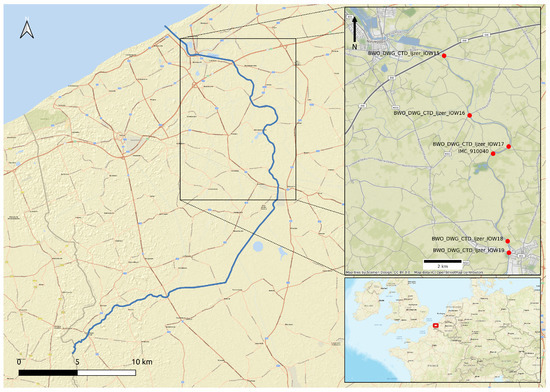
Figure 11.
An overview of the Yser river in the North West of Belgium and a more detailed view of the station placement used in the queries.
Before modelling the river as a (temporal) graph, we need to explore the data. This will allow, for example, to categorize the data provided by the sensors. We explain this next.
7.1. Data Exploration
We carry out the analysis both globally (that means, considering the thirty-seven stations) and locally (considering the values of each single station). We explain this next.
7.1.1. Global Analysis
The readings from thirty-seven stations are put together to analyze the distribution of the electric conductivity. Each record from the data set has a timestamp and a value that represents the ec value from the water at that time. The Yser river traverses different areas. The water temperature influences the values of conductivity. Thus, in order make values comparable, all measurements are corrected considering the water temperature, meaning that for all time series, the values are recalculated to the so-called “EC25”, meaning that the EC parameter is normalized corresponding a water temperature of 25 degrees Celsius. Table 1 describes the classic statistical values for the data obtained from the sensors. The total number of readings is 93,908 with a minimum value of 0 µS/cm and a maximum of 66,907.53 µS/cm.

Table 1.
EC25 variable: basic statistics. All values in µS/cm, except the count.
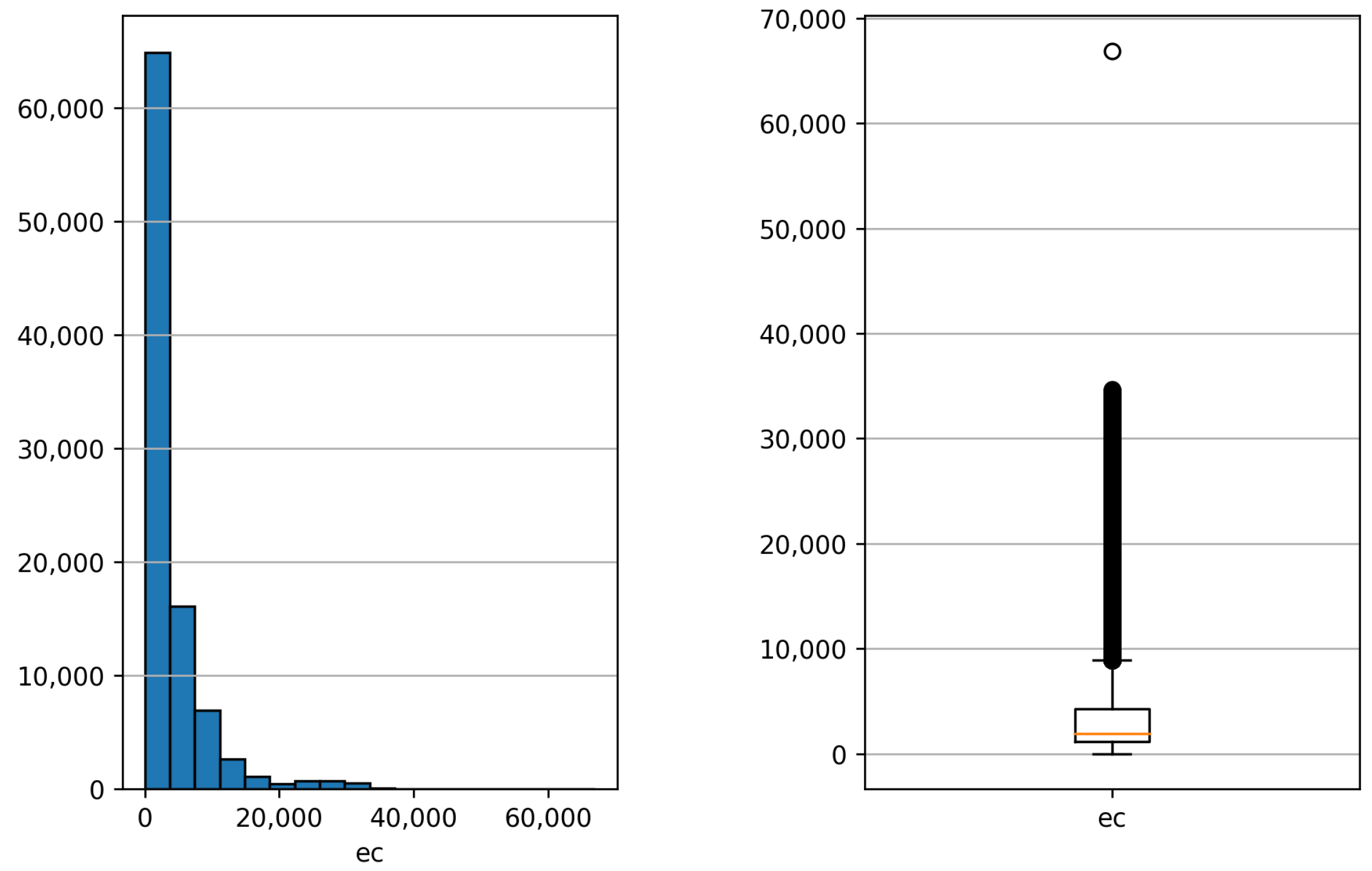
Our main goal here is to determine the thresholds that will be used for categorizing the data, since our technique requires using categorical variables. Thus, we build a histogram shown on the left-hand side of Figure 12. We used the classic Sturges formula to estimate the number of bins: , where N is the total number of values. This produces eighteen bins. We can see that most of the values fall in the first bin (from 0 µS/cm to 3717.08 µS/cm). This can also be seen in the boxplot on the right-hand side of Figure 12, that shows 9432 values considered as outliers (above the 8878.74 µS/cm), which represent approximately of the readings.
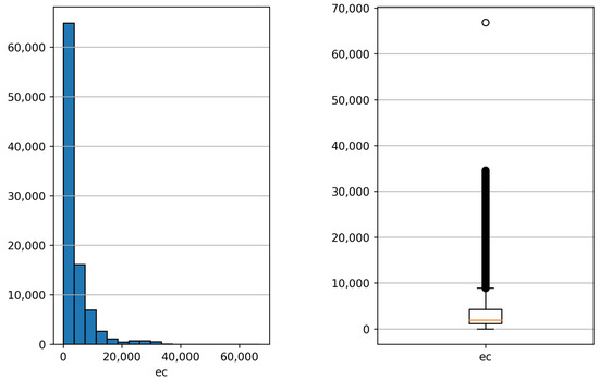
Figure 12.
Electric conductivity histogram and boxplot.
7.1.2. Local Analysis
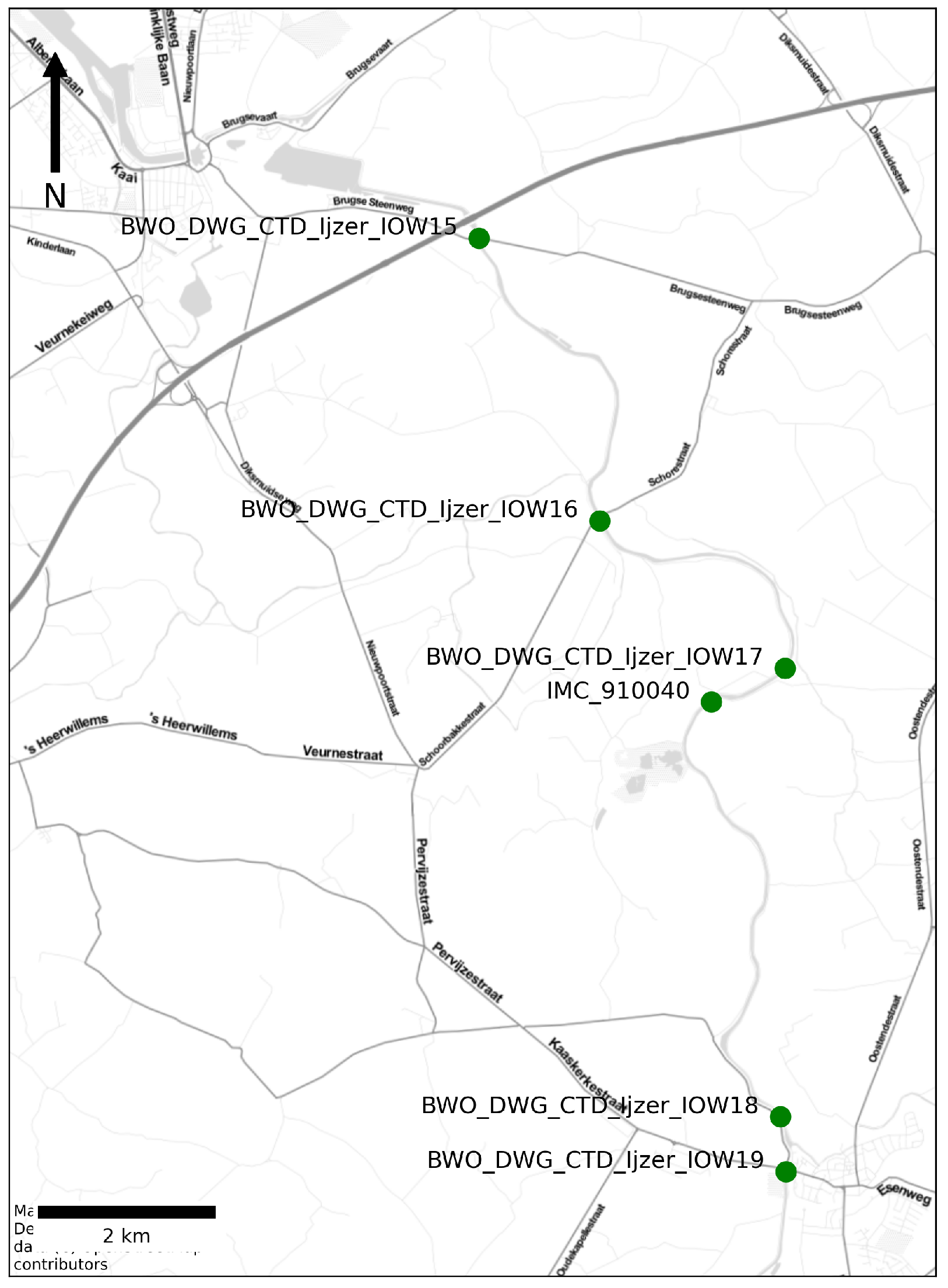
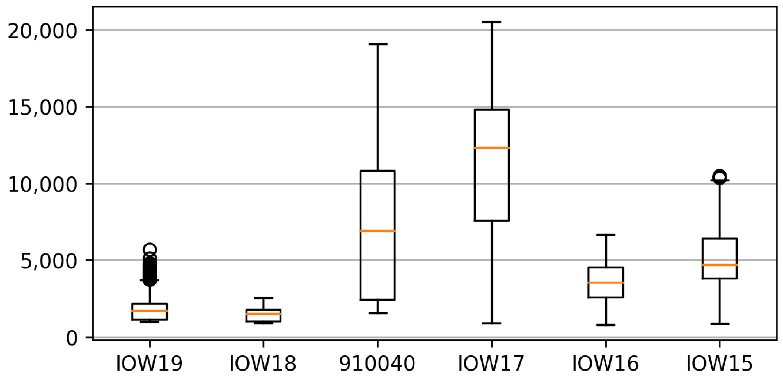
The data distribution at each station in the data set (that means, considering only the data for the station) may differ from the global one, even if the values are corrected to EC25. In this case, we want to study the behaviour of the variable, so a subset of six contiguous stations will be considered. These stations are depicted in Figure 13. In what follows we will refer to these stations as , , , , , respectively, although the actual names are longer (e.g., ). Table 2 shows these stations and the local statistical for their values. Also, for each station, a boxplot is depicted in Figure 14. It can be seen that except for stations and , the median value of the ec variable is higher than the global median and all of them show different distributions.
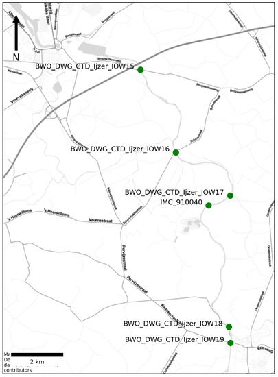
Figure 13.
Stations on the Yser river between the cities of Diksmuide and Nieuwpoort.

Table 2.
EC25 variable: data description per station (values in µS/cm).
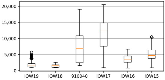
Figure 14.
Variable ec: boxplot per station.
7.2. Model Construction and Categorization of Variables
In order to be able to build the temporal graph that models the Yser river, we need to transform the time series consisting in continuous values into a time series of categorical values. Converting the continuous values of a variable into categories associated with value intervals is not a trivial task, since we must define the category thresholds. This can be done based on expert advice and/or on the distribution of the variable. In this work, the second approach is chosen. Also, as mentioned in the previous section, we can define the categories based on global values or on values relative to each station. For example, if the values registered in neighbouring stations are in very different ranges, what we consider as High for one station may be Low for another one. This strongly impacts of the paths that are discovered when querying the graph. In what follows, we present the study following the two criteria. We first show how to categorize the variables and build the graph considering the global definition of thresholds (Section 7.2.1), while the local definition of thresholds and the construction of the graph based on this categorization is addressed in Section 7.2.3.
7.2.1. Categorization of Variables Using Global Thresholds
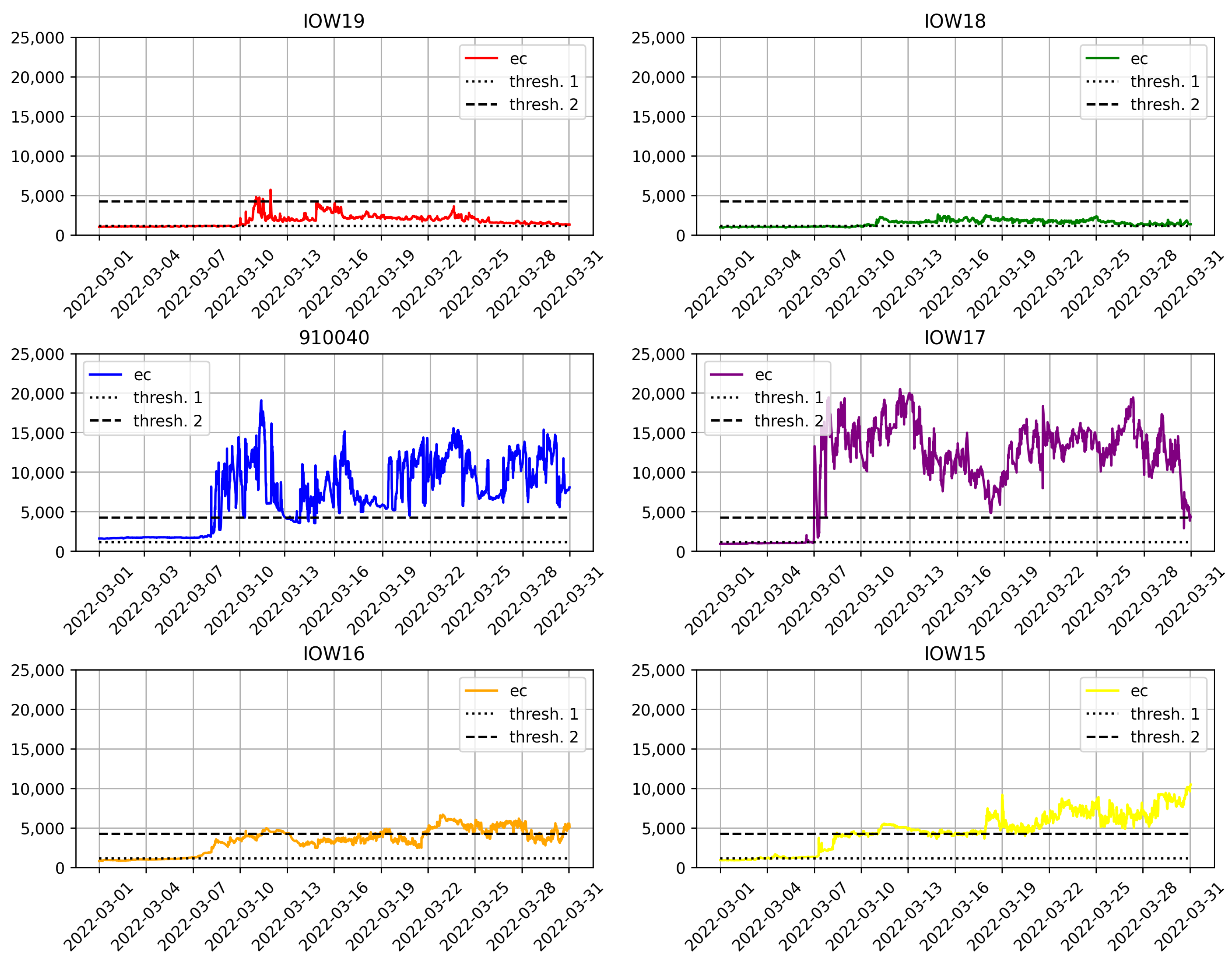
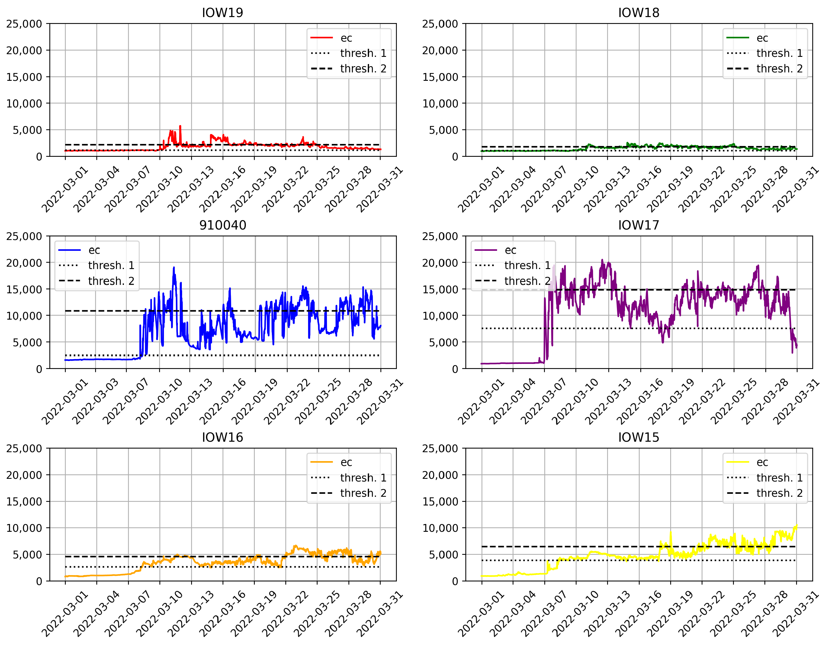
We choose two thresholds in order to divide the values in three categories: 0, 1 and 2, (for Low, Medium and High), based on the global statistics shown in Table 1. Figure 15 shows the data plot for each of the six stations we will analyze, for the month under analysis, ordered from left to right and up to down, in the water-flow direction (i.e., and are the farthest and closest to the sea, respectively). Along with the variable plot, two thresholds (in black) are shown in dashed lines, corresponding to the quantiles (1128.24 µS/cm) and (4228.44 µS/cm) of the global data. Later in the paper we study the impact of this choice, with respect to the local data.
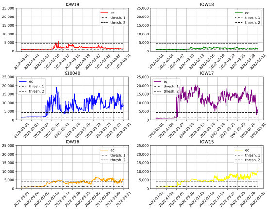
Figure 15.
Variable plot during March with two thresholds: quantiles (thresh 1) and (thresh 2).
7.2.2. Construction of the Graph Using Global Categorization
Once the thresholds are determined, the “base” graph can be built. This graph contains one node for every segment (as explained in Section 3), and some of the segments contain sensors (that is, they are sensor nodes in our notation). However, due to the geographical location with respect to the river segments, there are segments with more than one station. In this case, we create a sensor node for each of the station in the same segment, and connect them via a edge preserving the water flow direction. Every segment node has a property that represents the river segment identifier (called vhas in the data set). This identifier is used to associate the stations with their location in the river. Thus, in case that more than one station were associated to a segment, they will have the same vhas value. However, as in the original TGraph, every node (Segment or Sensor) has a property that uniquely identifies it ().
For every station that measures the ec variable, an attribute node is created and connected to its sensor node. Finally, the values of the sensor readings are categorized and grouped in maximal non-overlapping ordered intervals. Figure 16 shows the resulting graph for the nodes corresponding to Figure 13. Blue-filled nodes are sensor nodes. Yellow nodes are attribute nodes and green nodes are value nodes. The number printed on the value nodes corresponds to their category. We do not show the intervals here because in many cases, the list is too long. For example, for station , the intervals for category 2 are [2022-03-07 04:30–2022-03-07 06:30),[2022-03-07 13:00–2022-03-31 13:00),[2022-03-31 13:30–2022-03-31 22:30),[2022-03-31 22:45–2022-04-01 00:00). The resulting graph contains 545 segment nodes, 41 attribute nodes, 123 value nodes and 798 edges, where 552 are labeled as . The size of the Neo4j database is 1.6 MB.

Figure 16.
Neo4j Graph using the categorization based on global thresholds.
7.2.3. Categorization of Variables Using Local Thresholds
In Section 7.2.1 we used global statistics to define the thresholds for categorization of the values of the variables. We have also commented that it would be possible that using global variables have an impact in the analysis results if there is enough difference in the values in different stations. We study this impact next.
Similarly to Section 7.2.1, we define two thresholds for the discretization of the values into three categories: 0, 1, 2 (Low, Medium and High), but now these values will correspond to the quantiles and of every individual station. Figure 17 shows a plot of the values for the stations under study. We also show two thresholds, in dashed lines, corresponding to the first and second thresholds.
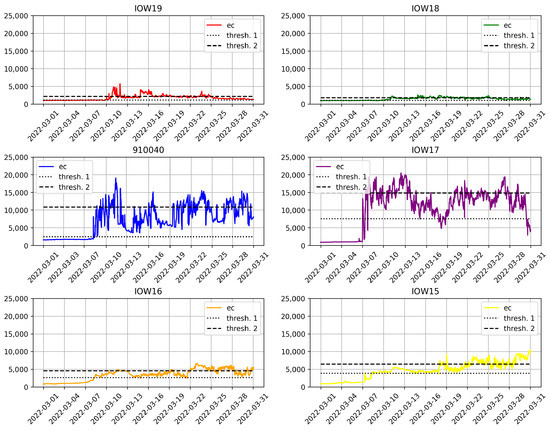
Figure 17.
Variable plot during March with two thresholds: quantiles and of every station.
7.2.4. Construction of the Graph Using Local Categorization
We now build the graph using the thresholds defined in the previous section. Thus, the resulting intervals and categories are different than the ones obtained with global categorization. For example, in the global case, station has two categories, while in the local case, it has all three possible categories.
We can see the resulting graph in Figure 18. The reader can compare against the graph built based on the categorization computed using local thresholds. The resulting graph contains 545 segment nodes, 41 attribute nodes, 164 value nodes and 798 edges, where 552 are labeled as . The size of the resulting Neo4j database is 1.9 MB.

Figure 18.
Neo4j Graph using the categorization based on local thresholds.
7.3. Querying the Transportation Network Graph with T-GQL
Over the graphs built in the previous sections, we are ready now to express queries that can compute the paths studied in this paper. These queries can then be used by the domain experts to draw conclusions about the water quality, and the impact that different events may have on the quality parameters. Again, we divide the study in terms of the categorizations of Section 7.2. We will denote both graphs in Figure 16 and Figure 18 as global and local graphs, respectively. Also, for simplicity, we define a default value of three days for the delay parameter , so we omit it in the function calls.
7.4. Querying the Global Graph
We start with a query asking for (forward and backwards) Flow Paths.
Query 1.
Find the Flow Paths starting from Category 0 between 9 March and 11 March, starting from station . Consider also the paths such that the category continuously increases.
1 SELECT p.path, p.intervals
2 MATCH (p1:Sensor), (p2:Sensor),
3     p=FPath((p1) - [f:flowsTo∗2..6] -> (p2),
4     ’2022-03-09 16:00’,’2022-03-11 00:00’,’ec’,’up’,’0’)
5 WHERE p1.Name = ’BWO_DWG_CTD_Ijzer_IOW19’
This query asks for the generalized FPs introduced in Section 5.5, thus, we include the “up” parameter in the T-GQL query. The function FPath computes the paths with lengths between two and six, during the requested interval. The result below (returned by the query engine in JSON format), shows that, starting from station , there is a path comprising three stations.
{
  "path": {
  "name": "BWO_DWG_CTD_Ijzer_IOW19",
  "value": "0",
  "attribute": "ec"},
{
  "name": "BWO_DWG_CTD_Ijzer_IOW18",
  "value": "1",
  "attribute": "ec"},
{
  "title": "Segment",
  "id": 506},
{
  "name": "IMC_910040",
  "value": "1",
  "attribute": "ec"
}
],
  "intervals": [
    "2022-03-09 16:15 - 2022-03-09 23:30",
    "2022-03-09 23:30 - 2022-03-10 02:45",
    "2022-03-10 14:15 - 2022-03-10 14:30"
    ]
  ]
}
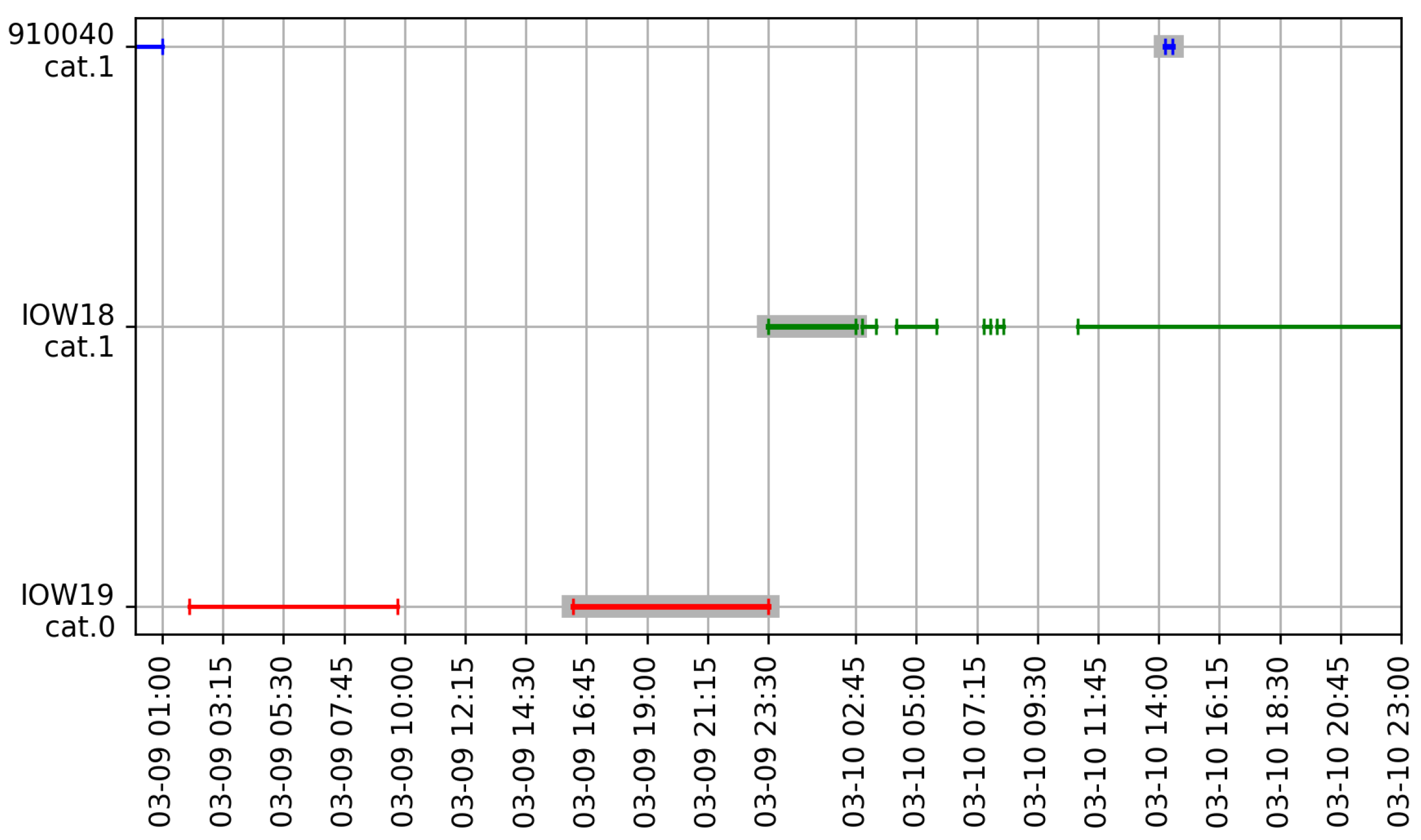
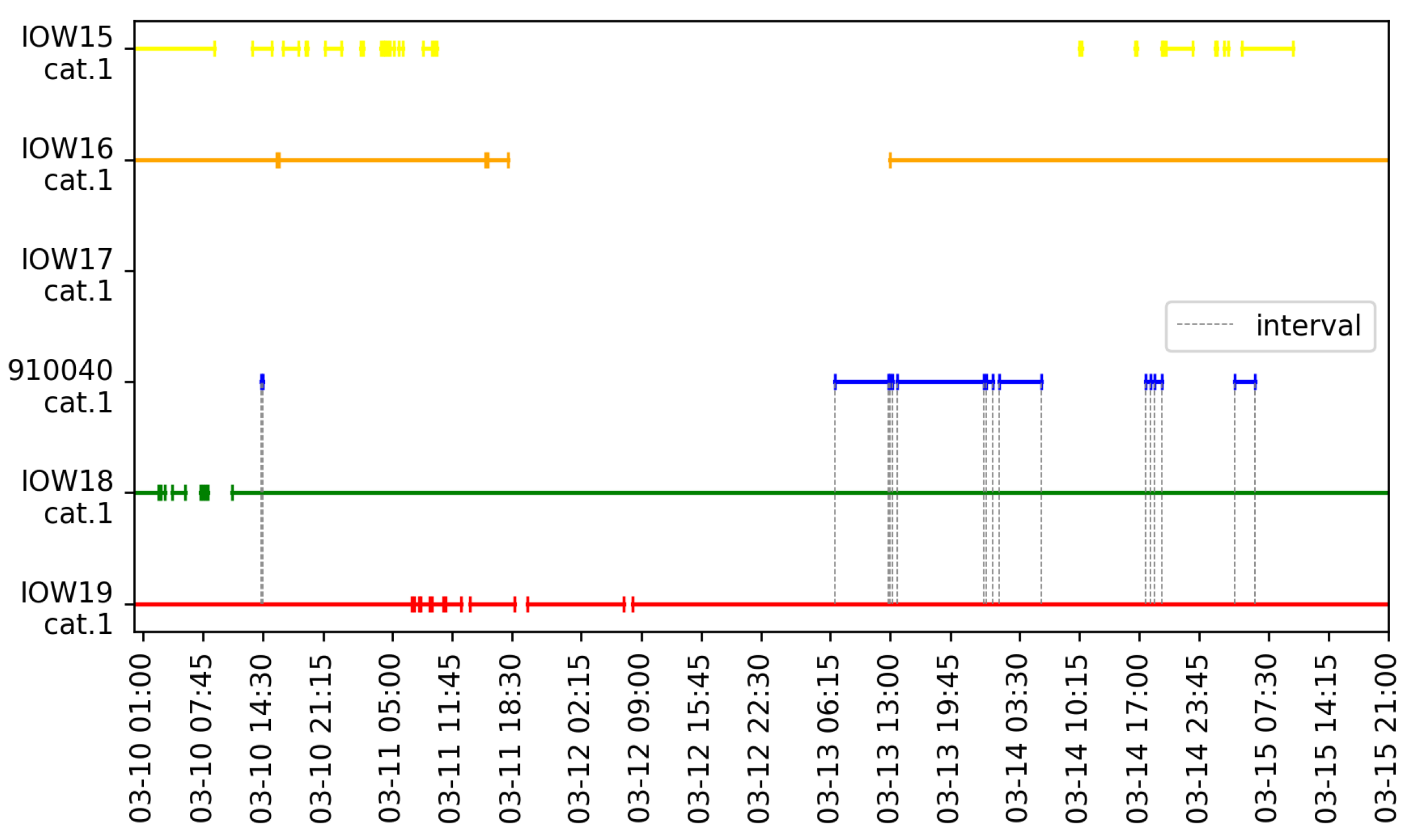
It can be seen that the number of intervals returned by the FPath function corresponds to the number of stations in the solution path. In this case we can see three intervals, corresponding to the three stations in the query result: The interval “2022-03-09 16:15–2022-03-09 23:30” corresponds to the station , interval “2022-03-09 23:30–2022-03-10 02:45” to and interval “2022-03-10 14:15–2022-03-10 14:30” to . We can also see that the start time of every interval is greater than the one corresponding to the previous station. Figure 19 shows this graphically. The figure represents, for each station and its returned category of , a line indicating the time periods when each station registered each value. For example, a red line indicates the periods when station registered a value within category 0. We use this figure to indicate the FP returned by the query. We can see the three intervals of the FP, depicted in gray over three lines for each station, within a time window that ranges from 9 March through 10 March.
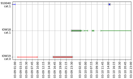
Figure 19.
Flow Path query result for Query 1.
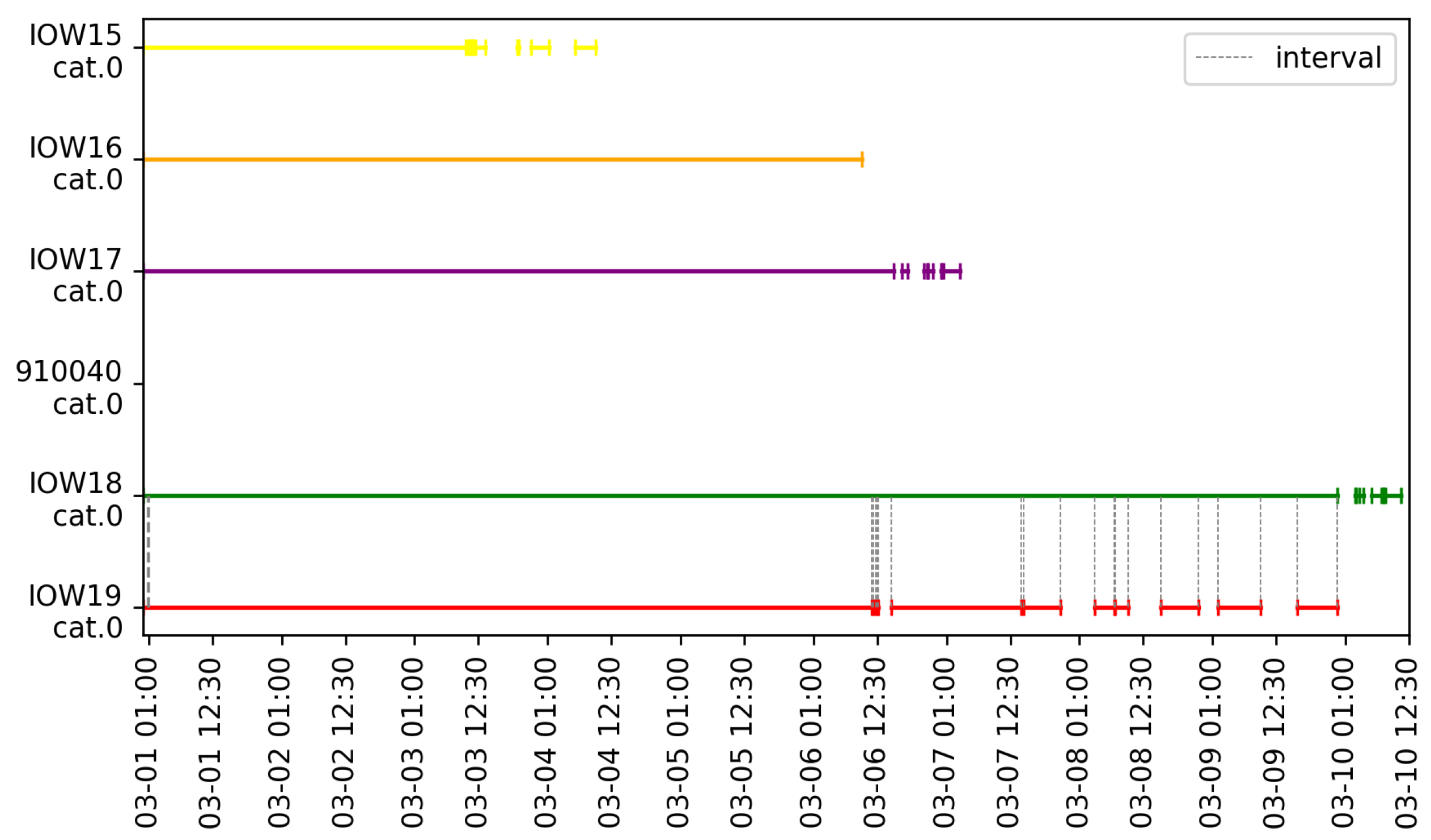
We would like to remark that computing paths using queries like Query 1 (which are rather intuitive for non-expert SQL users), allows discovering, at a glance, a structure that otherwise remains hidden in plots like the ones in Figure 15.
In the plot for station of Figure 15, we can see a raise of the on 8 March. To check whether this effect is propagating backwards through the rest of the stations, the following query is formulated.
Query 2.
Compute the Backwards Flow Paths starting at station between 4 March and 9 March. Also consider the continuously increasing pattern.
This query asks for the generalized FPs introduced in Section 5.5, thus, we include the “up” parameter in the T-GQL query.
1 SELECT p.path, p.intervals
2 MATCH (p1:Sensor), (p2:Sensor),
3     p=FPath((p1) <- [f:flowsTo∗2..6] - (p2),
4     ’2022-03-04 01:20’,’2022-03-09 00:00’,’ec’,’up’,’0’)
5 WHERE p1.Name = ’BWO_DWG_CTD_Ijzer_IOW15’
This query calls the FPath function to get those paths where the value of ec is rising and propagating backwards. The path can contain between 2 and 6 sensors. Although the function that is called is the same as in Query 1, the arrow in the MATCH pattern is written in the reverse direction, indicating that we look for paths propagating in the direction contrary to the flow. That is, we have a parameter propagating opposite to the river flow. The resulting path of length 4 is shown below in JSON format.
{
  "path": [
    {
    "name":  "BWO_DWG_CTD_Ijzer_IOW15",
    "value": "0",
    "attribute": "ec"
    },
    {
    "name": "BWO_DWG_CTD_Ijzer_IOW16",
    "value": "1",
    "attribute": "ec"
    },
    {
    "name": "BWO_DWG_CTD_Ijzer_IOW17",
    "value": "1",
    "attribute": "ec"
    },
    {
    "name": "IMC_910040",
    "value": "2",
    "attribute": "ec"
    }
  ],
  "intervals": [
    [
      "2022-03-04 06:00 - 2022-03-04 09:45",
      "2022-03-06 09:45 - 2022-03-10 16:00",
      "2022-03-06 15:30 - 2022-03-06 17:00",
      "2022-03-08 09:00 - 2022-03-08 09:15"
    ]
   ]
}
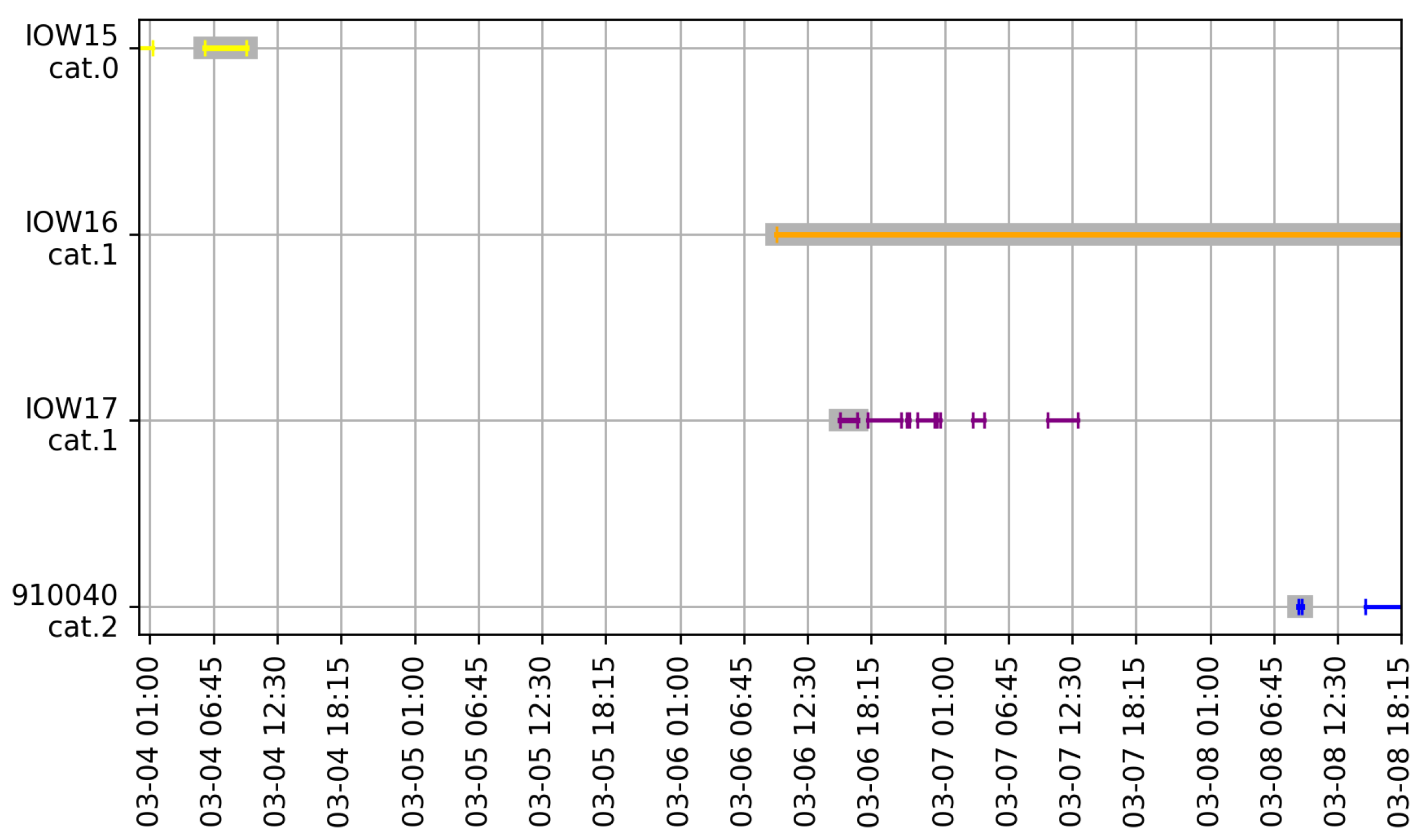
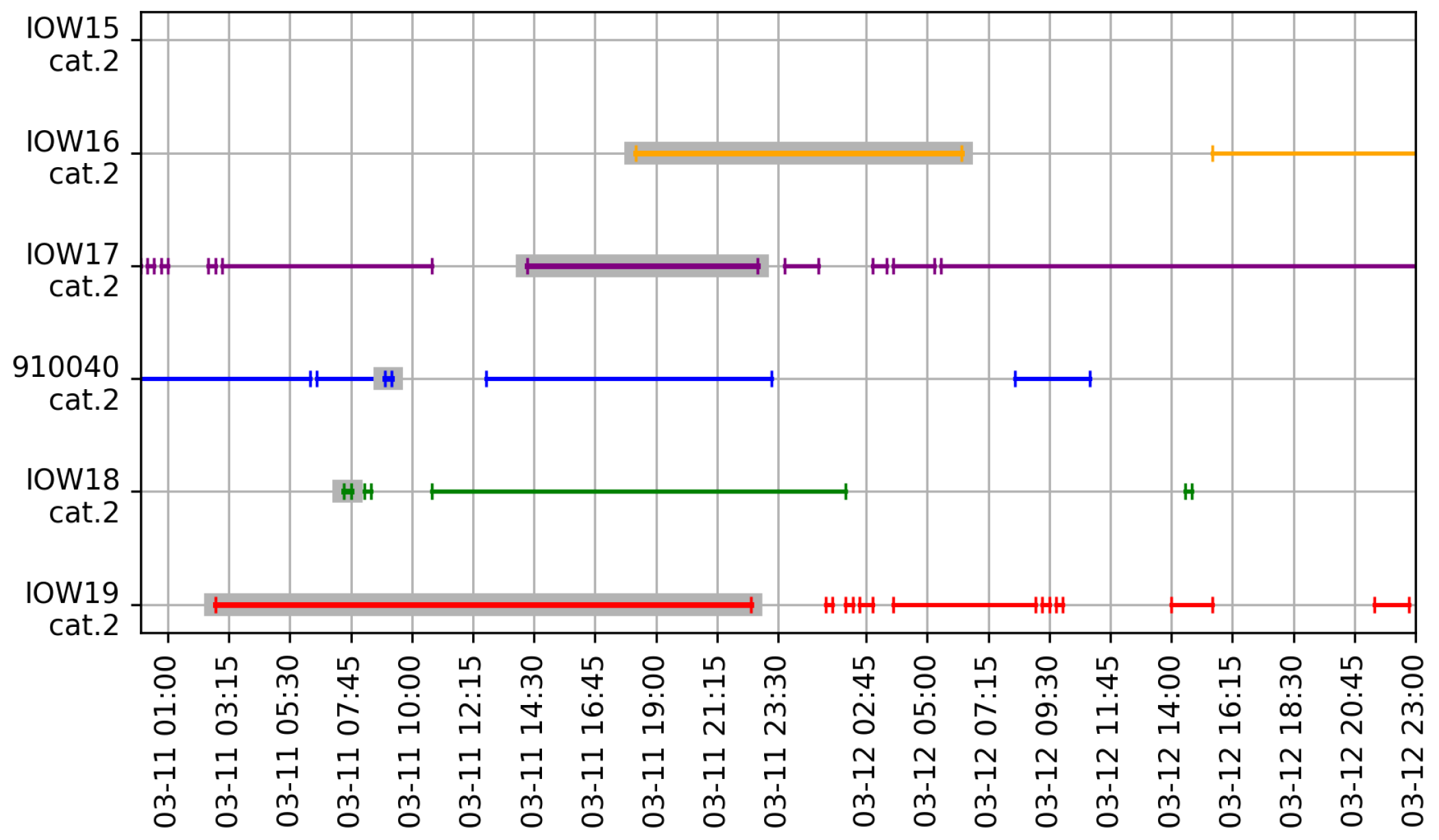
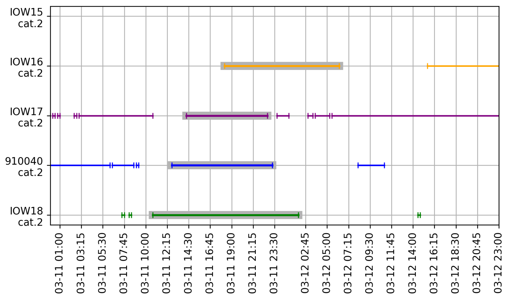
We can see that the resulting path contains four sensor nodes and their values rise from 0 to 2. The BF Paths are somehow tricky in the following sense: note that the first station in the path (which represents a path followed by the pollutant) is actually the last one in downstream direction, that is, in the direction of the river flow. This is the meaning of the Backwards Flow Paths. As in the previous query, there is an interval for each station. The interval returned for the last node representing station , corresponds to the peaks present in Figure 15. The next station in upstream direction () has no interval for ec = 2 in the returned periods; therefore, since the value must be 2 or greater (because we ask for increasing values), the algorithm stops here. These intervals can be seen in Figure 20 which has the same interpretation than in the previous query. Note that the river flows from station up to , and in gray over the lines we can see, within a time window that ranges from 4 March to 8 March, that the values of the categories for ec increase in the opposite direction (downwards in the picture).

Figure 20.
Query result for Query 2.
We now move to look for TNCPs which involve the stations under study. The query below aims at discovering CPs in these stations.
Query 3.
Compute the CPs for , together with the intervals when they occurred, during 1 March to 9 March at 23:59.
The T-GQL query is written:
1 SELECT p.path, p.intervals
2 MATCH (p1:Sensor), (p2:Sensor),
3     p=TNCPath((p1) - [f:flowsTo∗2..6] -> (p2),
4     ’2022-03-01 00:00’,’2022-03-09 23:59’,’ec’,’=’,’0’)
5 WHERE p1.Name = ’BWO_DWG_CTD_Ijzer_IOW19’
The query calls the function (Transportation Network Continuous path) to get those paths where the value of ec is continuously equal to 0. The result in JSON format returned by the query engine is:
[
{
  "path": [
    {
    "name": "BWO_DWG_CTD_Ijzer_IOW19",
    "vhas": "6033639",
    "value": "0",
    "attribute": "ec"
    },
    {
    "name": {
    "name": "BWO_DWG_CTD_Ijzer_IOW18",
    "vhas": "7058471",
    "value": "0",
    "attribute": "ec"
    }
  ],
  "intervals": [
    [
      "2022-03-01 00:00 - 2022-03-06 11:30",
      "2022-03-06 11:45 - 2022-03-06 12:15",
      "2022-03-06 12:30 - 2022-03-06 12:45",
      "2022-03-06 15:00 - 2022-03-07 14:30",
      "2022-03-07 15:00 - 2022-03-07 21:30",
      "2022-03-08 03:45 - 2022-03-08 07:15",
      "2022-03-08 07:30 - 2022-03-08 09:45",
      "2022-03-08 15:45 - 2022-03-08 22:30",
      "2022-03-09 02:00 - 2022-03-09 09:45",
      "2022-03-09 16:15 - 2022-03-09 23:30"]
    ]
  ]
}
]
In this case, the interpretation of the intervals returned by the function differs from the one returned by the FPath function. Here, the intervals represent the intersection, i.e., the times when the operation (in this case, the value = 0) was valid for all the stations simultaneously. Thus, the number of stations in the returned path is not related to the number of the returned intervals, but indicates the number of CPs found. In this case, the first interval ranges from “2022-03-01 00:00 to 2022-03-06 11:30” because station stops registering the value 0 at 2022-03-06 11:30.
Figure 21 graphically shows the result. We can see that only the first two stations are involved, because, during the periods when the value held simultaneously in stations and , the value of ec in station was not zero. In that Figure, the vertical dashed lines show the intervals of the CPs over the stations and . We can see that we have several short CPs. Of course, the domain experts can give different interpretations to this result, and they can even coalesce or split the CPs using different parameters.

Figure 21.
TNCPs for Query 1 and = 0.
We now write the same query but for and a different time window.
1 SELECT p.path, p.intervals
2 MATCH (p1:Sensor), (p2:Sensor),
3     p=TNCPath((p1) - [f:flowsTo∗2..6] -> (p2),
4     ’2022-03-01 00:00’,’2022-03-16 23:00’,’ec’,’=’,’1’)
5 WHERE p1.Name = ’BWO_DWG_CTD_Ijzer_IOW19’
In this case we obtain two paths, one of them reaching station and the other one farther to station . We only show the results for the latter CP.
[
"2022-03-10 14:15 - 2022-03-10 14:30",
"2022-03-13 06:45 - 2022-03-13 12:45",
"2022-03-13 13:00 - 2022-03-13 13:15",
"2022-03-13 13:45 - 2022-03-13 23:30",
"2022-03-13 23:45 - 2022-03-14 00:30",
"2022-03-14 01:15 - 2022-03-14 06:00",
"2022-03-14 17:45 - 2022-03-14 18:15",
"2022-03-14 18:45 - 2022-03-14 19:30",
"2022-03-15 03:45 - 2022-03-15 06:00"
]
This result can be seen in Figure 22, where the first three stations have intersection but the fourth, has no value for = 1 in those periods.
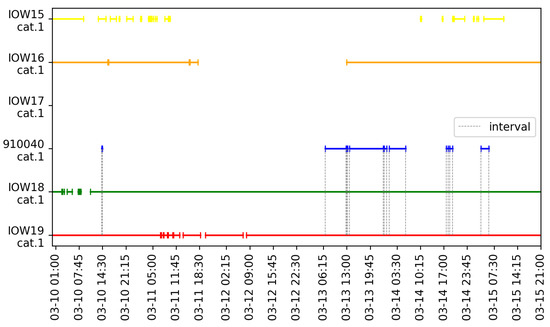
Figure 22.
Query result for Query 3 and = 1.
Finally, to check if there are continuous paths of value 2 (High), we write
1 SELECT p.path, p.intervals
2 MATCH (p1:Sensor), (p2:Sensor),
3     p=TNCPath((p1) - [f:flowsTo∗2..6] -> (p2),
4     ’2022-03-01 00:00’,’2022-03-31 23:00’,’ec’,’=’,’2’)
5 WHERE p1.Name = ’BWO_DWG_CTD_Ijzer_IOW19’
The result in this case contains no paths whatsoever, due to the fact that the second station, , never satisfies .
Querying the Local Graph
In the plot for station of Figure 15, a peak of the value can be seen on 11 March. We would like to check if this effect propagates forward through the rest of the stations. Thus, we write the following query:
Query 4.
Compute the Flow Paths, starting from station where the value of propagates forward with a path length between 2 and 6 sensor stations.
Again, in this case, we do not ask for increasing or decreasing FPs. The query reads:
1 SELECT p.path, p.intervals
2 MATCH (p1:Sensor), (p2:Sensor),
3     p=FPath((p1) - [f:flowsTo∗2..6] -> (p2),
4     ’2022-03-11 00:00’,’2022-03-13 00:00’,’ec’,’=’,’2’)
5 WHERE p1.Name = ’BWO_DWG_CTD_Ijzer_IOW19’
Below we show the longest of the resulting paths, in JSON format.
{
  "path": {
  "name": "BWO_DWG_CTD_Ijzer_IOW19",
  "value": "2",
  "attribute": "ec"},
{
  "name": "BWO_DWG_CTD_Ijzer_IOW18",
  "value": "2",
  "attribute": "ec"},
{
  "title": "Segment",
  "id": 506},
{
  "name": "IMC_910040",
  "value": "2",
  "attribute": "ec"
},
{
  "name": "BWO_DWG_CTD_Ijzer_IOW17",
  "value": "2",
  "attribute": "ec"},
{
  "name": "BWO_DWG_CTD_Ijzer_IOW16",
  "value": "2",
  "attribute": "ec"}
],
  "intervals": [
    "2022-03-11 02:45 - 2022-03-11 22:30",
    "2022-03-11 07:30 - 2022-03-11 07:45",
    "2022-03-11 09:00 - 2022-03-11 09:15",
    "2022-03-11 14:15 - 2022-03-11 22:45",
    "2022-03-11 18:15 - 2022-03-12 06:15"
    ]
  ]
}
Like in Query 1, the number of returned intervals corresponds to the number of stations in the path (in the same order). For example, interval “2022-03-11 02:45–2022-03-11 22:30” corresponds to station , “2022-03-11 07:30–2022-03-11 07:45” to , and so on.
According to this result, the value = 2 starts at station on 11 March at 02:45, as then propagates through the stations, arriving at station on 11 March at 18:15. Figure 23 shows the resulting intervals marked in grey over the lines representing the values of the categories (in this case, the value is 2 for all stations) for each station at different intervals. We look for Flow Paths, thus we can see that the grey lines move forward in time and also in the direction of the flow, that starts at and ends at . Since station has not registered a value in category 2 during the time window, it does not appear in the result.
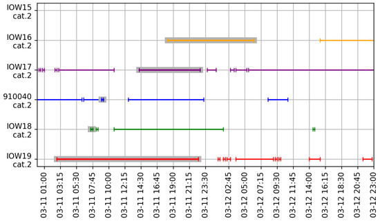
Figure 23.
Flow Paths for Query 4.
Figure 23 also shows that the interval obtained for station is very small (15 min) and one could expect to obtain the longer one that starts at 10:15. This is due to the way algorithm picks the interval closest to the previous station. This can be corrected changing some parameters, and it is left as the domain expert’s task.
Consider now a similar query, but starting at station .
Query 5.
Compute the Flow Paths starting at station , where the value of and propagating forward, with a path length between 2 and 6 sensor stations, in a time window between 11 March at 10:00 and 13 March at 00:00.
1 SELECT p.path, p.intervals
2 MATCH (p1:Sensor), (p2:Sensor),
3     p=FPath((p1) - [f:flowsTo∗2..6] -> (p2),
4     ’2022-03-11 10:00’,’2022-03-13 00:00’,’ec’,’=’,’2’)
5 WHERE p1.Name = ’BWO_DWG_CTD_Ijzer_IOW18’
Again for brevity we only show the longest of the resulting paths.
{
  "path": {
  "name": "BWO_DWG_CTD_Ijzer_IOW18",
  "value": "2",
  "attribute": "ec"},
{
  "title": "Segment",
  "id": 506},
{
  "name": "IMC_910040",
  "value": "2",
  "attribute": "ec"
},
{
  "name": "BWO_DWG_CTD_Ijzer_IOW17",
  "value": "2",
  "attribute": "ec"},
{
  "name": "BWO_DWG_CTD_Ijzer_IOW16",
  "value": "2",
  "attribute": "ec"}
],
  "intervals": [
    "2022-03-11 10:45 - 2022-03-12 02:00",
    "2022-03-11 12:45 - 2022-03-11 23:15",
    "2022-03-11 14:15 - 2022-03-11 22:45",
    "2022-03-11 18:15 - 2022-03-12 06:15"
    ]
  ]
}
Figure 24 shows the resulting intervals shaded in grey over the lines representing the values of the categories (again,the value is 2 for all stations) for each station at different intervals. We can see that choosing a different time window yields longer intervals than with the longer window in Query 4.
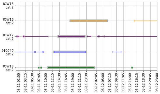
Figure 24.
Flow Paths for Query 5.
We now use the local thresholds to compute the Backwards Flow paths
Query 6.
Compute the Flow Backwards paths between 8 March and 13 March, starting at station .
The T-GQL query is written as follows.
1 SELECT p.path, p.intervals
2 MATCH (p1:Sensor), (p2:Sensor),
3     p=FPath((p1) <- [f:flowsTo∗2..6] - (p2),
4     ’2022-03-08 00:00’, ’2022-03-13 00:00,’ec’,’up’,’1’)
5 WHERE p1.Name = ’BWO_DWG_CTD_Ijzer_IOW15’
Below, we show the result of the longest path found. Note, again, that the path starts with the station closest to the sea (that is, the last station in the downstream flow), since we are analyzing the backwards movement of the pollutant.
{
  "path": {
  "name": "BWO_DWG_CTD_Ijzer_IOW15",
  "value": "1",
  "attribute": "ec"},
{
  "name": "BWO_DWG_CTD_Ijzer_IOW16",
  "value": "2",
  "attribute": "ec"},
{
  "name": "BWO_DWG_CTD_Ijzer_IOW17",
  "value": "2",
  "attribute": "ec"},
{
  "name": "IMC_910040",
  "value": "2",
  "attribute": "ec"},
{
  "title": "Segment",
  "id": 506},
{
  "name": "BWO_DWG_CTD_Ijzer_IOW16",
  "value": "2",
  "attribute": "ec"},
{
  "name": "BWO_DWG_CTD_Ijzer_IOW15",
  "value": "2",
  "attribute": "ec"}
],
  "intervals": [
   "2022-03-08 13:00 - 2022-03-08 13:30",
   "2022-03-10 16:00 - 2022-03-10 16:15",
   "2022-03-10 18:15 - 2022-03-10 18:30",
   "2022-03-10 21:15 - 2022-03-10 21:45",
   "2022-03-11 07:30 - 2022-03-11 07:45",
   "2022-03-12 01:15 - 2022-03-12 01:30"
    ]
  ]
}
The resulting paths can be seen in Figure 25. Here, the first interval, “2022-03-08 13:00–2022-03-08 13:30”, corresponds to station (that is, the first station in upstream direction of the pollutant), the second, “2022-03-10 16:00–2022-03-10 16:15”, to station , and so on. In this case, all of the returned intervals are very short (between 15 and 30 min long). Deciding whether or not these are meaningful paths is a task of the domain experts.
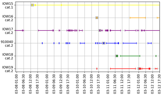
Figure 25.
Backwards Flow Path result for Query 6.
We now move again to Continuous Path queries, now over the graph built with local thresholds.
Query 7.
Compute all Continuous Paths with value 2 in the six stations under study, during 24 March, starting at station .
1 SELECT p.path, p.intervals
2 MATCH (p1:Sensor), (p2:Sensor),
3     p=TNCPath((p1) - [f:flowsTo∗2..6] -> (p2),
4     ’2022-03-24 00:00’,’2022-03-25 00:00’,’ec’,’=’,’2’)
5 WHERE p1.Name = ’BWO_DWG_CTD_Ijzer_IOW19’
The longest path found (considering the number of returned nodes) is shown below.
[
{
  "path": [
    {
    "name": "BWO_DWG_CTD_Ijzer_IOW19",
    "vhas": "6033639",
    "value": "2",
    "attribute": "ec"
    "vhas": "6033639"
    },
    {
    "name": {
    "name": "BWO_DWG_CTD_Ijzer_IOW18",
    "vhas": "7058471",
    "value": "2",
    "attribute": "ec"
    },
    {
  "vhas": "7058475"
    },
    {
    "name": "IMC_910040",
    "vhas": "6033616",
    "value": "2",
    "attribute": "ec"
    },
    {
    "name": "BWO_DWG_CTD_Ijzer_IOW17",
    "vhas": "6033616",
    "value": "2",
    "attribute": "ec"
    },
    {
    "name": "BWO_DWG_CTD_Ijzer_IOW16",
    "vhas": "6033616",
    "value": "2",
    "attribute": "ec"
    },
    {
    "name": "BWO_DWG_CTD_Ijzer_IOW15",
    "vhas": "6033616",
    "value": "2",
    "attribute": "ec"
    }
],
  "intervals": [
    [
    "2022-03-24 16:15 - 2022-03-24 16:30",
    "2022-03-24 18:00 - 2022-03-24 19:30",
    "2022-03-24 19:45 - 2022-03-24 20:15",
    "2022-03-24 20:45 - 2022-03-24 21:00"
    ]
  ]
}
]
This query returns a path of six sensors because between ‘2022-03-24 00:00’ and ‘2022-03-25 00:00’, there were four times in which all the six stations shared a value of 2 for . These times are “2022-03-24 16:15–2022-03-24 16:30”, “2022-03-24 18:00–2022-03-24 19:30”, “2022-03-24 19:45–2022-03-24 20:15” and “2022-03-24 20:45–2022-03-24 21:00”. They are depicted in Figure 26 with vertical gray lines. We can see that although we have shown that it was not possible to find a CP using global thresholds, with local thresholds the result is completely different and four CPs were found as the intervals in the result above show.
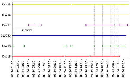
Figure 26.
CPs result for Query 7 using local thresholds and .
7.5. Execution Times
Although the paper is not oriented to deal with efficiency at this time, we report the running times of the queries above. Queries 1 to 7 were run on an Intel(R) Core(TM) i7-7500U CPU@ 2.70 GHz with a RAM of 16 GB. Table 3 reports, for each query, the number of paths returned and the total execution time (including translation), expressed in miliseconds.

Table 3.
Query execution times.
8. Discussion and Future Work
In this paper, we have considered transportation networks that are equipped with sensors and we have shown how graph databases can be used to store, view, query and analyse such data. In particular, we have used temporal graph databases and temporal graph query languages for this purpose and we have illustrated how various types of path queries can be used to discover interesting patterns in the time-series data that are produced by sensors.
In Section 7, we presented a real-world use case to illustrate how interesting information can be extracted from a data set that concerns a part of the Belgian river system that is equipped with sensors. Here, we model this river system as a temporal graph and implement it using real data provided by the sensors. We have discovered interesting temporal paths based on the electric conductivity parameter, that can be used in a decision support environment, by hydrological experts like water managers, for analyzing water quality across time.
We want to remark that the outcome of several of the experiments that we have presented depends on parameters or choices such as the way we categorize the time-series data, the way we define intervals and even on the definition of certain path classes. When, for example, a different method of dividing time-series values in categories would be used, different paths would result from the data. We see the choice of these procedures as parameters that can be presented to domain experts, such as hydrologist, that can be experimented with and can be fine-tuned. In the end, our system presents potentially interesting patterns that are present in huge sensor-produced data sets and it is up to the domain expert to attach an interpretation to them. In that sense, we see the formalism and system that we have presented as part of a decision support system that helps experts to discover knowledge in large data sets.
In conclusion, we also remark that the case of river systems equipped with sensors, that we present in this paper, is just one example. As a further or next example, we see road networks equipped with various sensors (even with camera images). But there are also the examples of power grids (in which electricity is transported), computer networks (in which electricity information is transported) and biological networks (in which nutrition is transported).
Author Contributions
Conceptualization, Alejandro Vaisman; methodology, Rik Hendrix and Bart Kuijpers; data curation, Erik Bollen; writing—original draft preparation, Valeria Soliani; writing—review and editing, Valeria Soliani and Bart Kuijpers. All authors contributed equally to this manuscript. All authors have read and agreed to the published version of the manuscript.
Funding
The research of Erik Bollen was supported by the Bijzonder Onderzoeksfonds (BOF) from UHasselt with reference BOF20OWB27 and by VITO with project reference 2010478. The research of Valeria Soliani is partially supported by the Bijzonder Onderzoeksfonds (BOF) from UHasselt with reference BOF22BL02 and by Project PICT 2017-1054, from the Argentinian Scientific Agency. Alejandro Vaisman was partially supported by Project PICT 2017-1054, from the Argentinian Scientific Agency.
Institutional Review Board Statement
Not applicable.
Informed Consent Statement
Not applicable.
Data Availability Statement
Data sharing not applicable.
Conflicts of Interest
The authors declare no conflict of interest.
References
- Akyildiz, I.; Su, W.; Sankarasubramaniam, Y.; Cayirci, E. A survey on sensor networks. IEEE Commun. Mag. 2002, 40, 102–114. [Google Scholar] [CrossRef]
- Bollen, E.; Hendrix, R.; Kuijpers, B.; Vaisman, A.A. Time-Series-Based Queries on Stable Transportation Networks Equipped with Sensors. ISPRS Int. J. Geo Inf. 2021, 10, 531. [Google Scholar] [CrossRef]
- Zhang, S.; Yao, Y.; Hu, J.; Zhao, Y.; Li, S.; Hu, J. Deep Autoencoder Neural Networks for Short-Term Traffic Congestion Prediction of Transportation Networks. Sensors 2019, 19, 2229. [Google Scholar] [CrossRef] [PubMed]
- Angles, R. The Property Graph Database Model. In Proceedings of the AMW CEUR Workshop Proceedings, Cali, Colombia, 21–25 May 2018; Volume 2100. Available online: CEUR-WS.org (accessed on 1 March 2019).
- Debrouvier, A.; Parodi, E.; Perazzo, M.; Soliani, V.; Vaisman, A.A. A model and query language for temporal graph databases. VLDB J. 2021, 30, 825–858. [Google Scholar] [CrossRef]
- Tansel, A.; Clifford, J.; Gadia, S. (Eds.) Temporal Databases: Theory, Design and Implementation; Benjamin/Cummings: San Francisco, CA, USA, 1993. [Google Scholar]
- Pagán, B.; Desmet, N.; Seuntjens, P.; Bollen, E.; Kuijpers, B. Data driven methods for real time flood, drought and water quality monitoring: Applications for Internet of Water. Eur. Geosci. Union Gen. Assem. 2020, EGU, 9291. [Google Scholar] [CrossRef]
- Havlik, D.; Schade, S.; Sabeur, Z.A.; Mazzetti, P.; Watson, K.; Berre, A.J.; Mon, J.L. From Sensor to Observation Web with Environmental Enablers in the Future Internet. Sensors 2011, 11, 3874–3907. [Google Scholar] [CrossRef]
- McCabe, M.F.; Rodell, M.; Alsdorf, D.E.; Miralles, D.G.; Uijlenhoet, R.; Wagner, W.; Lucieer, A.; Houborg, R.; Verhoest, N.E.C.; Franz, T.E.; et al. The future of Earth observation in hydrology. Hydrol. Earth Syst. Sci. 2017, 21, 3879–3914. [Google Scholar] [CrossRef]
- Reichstein, M.; Camps-Valls, G.; Stevens, B.; Jung, M.; Denzler, J.; Carvalhais, N.; Prabhat. Deep learning and process understanding for data-driven Earth system science. Nature 2019, 566, 195–204. [Google Scholar] [CrossRef] [PubMed]
- Bollen, E.; Hendrix, R.; Kuijpers, B.; Vaisman, A. Towards the Internet of Water: Using graph databases for hydrological analysis on the Flemish river system. Trans. GIS 2021, 25, 2907–2938. [Google Scholar] [CrossRef]
- Brouwers, J.; Peeters, B.; Van Steertegem, M.; Van Lipzig, N.; Wouters, H.; Beullens, J.; Demuzere, M.; Willems, P.; De Ridder, K.; Maiheu, B.; et al. MIRA Climate Report 2015; Technical Report; VMM: Aalst, Belgium, 2015. [Google Scholar]
- Gobin, A. Impact of heat and drought stress on arable crop production in Belgium. Nat. Hazards Earth Syst. Sci. 2012, 12, 1911–1922. [Google Scholar] [CrossRef]
- Jensen, S.K.; Pedersen, T.B.; Thomsen, C. Time Series Management Systems: A Survey. IEEE Trans. Knowl. Data Eng. 2017, 29, 2581–2600. [Google Scholar] [CrossRef]
- Lerner, A.; Shasha, D. AQuery: Query language for ordered data, optimization techniques, and experiments. In Proceedings of the 29th International Conference on Very Large Data Bases, VLDB 2003, Berlin, Germany, 9–12 September 2003; Selinger, P., Carey, M., Freytag, J., Abiteboul, S., Lockemann, P., Heuer, A., Eds.; Morgan Kaufmann: Burlington, MA, USA, 2003; pp. 345–356. [Google Scholar] [CrossRef]
- Sadri, R.; Zaniolo, C.; Zarkesh, A.M.; Adibi, J. A Sequential Pattern Query Language for Supporting Instant Data Mining for e-Services. In Proceedings of the VLDB 2001, 27th International Conference on Very Large Data Bases, Roma, Italy, 11–14 September 2001; Apers, P.M.G., Atzeni, P., Ceri, S., Paraboschi, S., Ramamohanarao, K., Snodgrass, R.T., Eds.; Morgan Kaufmann: Burlington, MA, USA, 2001; pp. 653–656. [Google Scholar]
- Seshadri, P.; Livny, M.; Ramakrishnan, R. The Design and Implementation of a Sequence Database System. In Proceedings of the VLDB’96, 22th International Conference on Very Large Data Bases, Mumbai (Bombay), India, 3–6 September 1996; Morgan Kaufmann: Burlington, MA, USA, 1996; pp. 99–110. [Google Scholar]
- Seshadri, P. Management of Sequence Data. Ph.D. Thesis, University of Wisconsin-Madison, CS Department, Madison, WI, USA, 1996. [Google Scholar]
- Weiss, C.H. Categorical Time Series Analysis. In Wiley StatsRef: Statistics Reference Online; John Wiley & Sons, Ltd: Hoboken, NJ, USA, 2018; pp. 1–8. [Google Scholar] [CrossRef]
- Weiss, C.H. Analyzing categorical time series in the presence of missing observations. Stat. Med. 2021, 40, 4675–4690. [Google Scholar] [CrossRef] [PubMed]
- Angles, R. A Comparison of Current Graph Database Models. In Proceedings of the ICDE Workshops, Arlington, VA, USA, 1–5 April 2012; pp. 171–177. [Google Scholar] [CrossRef]
- Robinson, I.; Webber, J.; Eifrem, E. Graph Databases; O’Reilly Media, Inc.: Newton, MA, USA, 2013. [Google Scholar]
- Angles, R.; Arenas, M.; Barceló, P.; Hogan, A.; Reutter, J.; Vrgoč, D. Foundations of Modern Query Languages for Graph Databases. ACM Comput. Surv. 2017, 50, 1–40. [Google Scholar] [CrossRef]
- Kuijpers, B.; Soliani, V.; Vaisman, A.A. Modeling and Querying Sensor Networks Using Temporal Graph Databases. In Proceedings of the New Trends in Database and Information Systems—ADBIS 2022 Short Papers, Doctoral Consortium and Workshops: DOING, K-GALS, MADEISD, MegaData, SWODCH, Turin, Italy, 5–8 September 2022; Springer: Berlin/Heidelberg, Germany, 2022; Volume 1652, pp. 222–231. [Google Scholar] [CrossRef]
- Kuijpers, B.; Ribas, I.; Soliani, V.; Vaisman, A.A. Indexing Continuous Paths in Temporal Graphs. In Proceedings of the New Trends in Database and Information Systems—ADBIS 2022 Short Papers, Doctoral Consortium and Workshops: DOING, K-GALS, MADEISD, MegaData, SWODCH, Turin, Italy, 5–8 September 2022; Springer: Berlin/Heidelberg, Germany, 2022; Volume 1652, pp. 232–242. [Google Scholar] [CrossRef]
- Francis, N.; Green, A.; Guagliardo, P.; Libkin, L.; Lindaaker, T.; Marsault, V.; Plantikow, S.; Rydberg, M.; Selmer, P.; Taylor, A. Cypher: An Evolving Query Language for Property Graphs. In Proceedings of the SIGMOD, Houston, TX, USA, 10–15 June 2018; ACM: New York, NY, USA, 2018; pp. 1433–1445. [Google Scholar] [CrossRef]
- Green, A.; Guagliardo, P.; Libkin, L.; Lindaaker, T.; Marsault, V.; Plantikow, S.; Schuster, M.; Selmer, P.; Voigt, H. Updating Graph Databases with Cypher. Proc. VLDB Endow. 2019, 12, 2242–2253. [Google Scholar] [CrossRef]
- Allen, J.F. Maintaining Knowledge about Temporal Intervals. Commun. ACM 1983, 26, 832–843. [Google Scholar] [CrossRef]
- Shuai, Z.; Yoon, S.; Oh, S.; Yang, M.H. Traffic Modeling and Prediction Using Sensor Networks: Who Will Go Where and When? Acm Trans. Sens. Netw. 2012, 9, 1–28. [Google Scholar] [CrossRef]
Disclaimer/Publisher’s Note: The statements, opinions and data contained in all publications are solely those of the individual author(s) and contributor(s) and not of MDPI and/or the editor(s). MDPI and/or the editor(s) disclaim responsibility for any injury to people or property resulting from any ideas, methods, instructions or products referred to in the content. |
© 2023 by the authors. Licensee MDPI, Basel, Switzerland. This article is an open access article distributed under the terms and conditions of the Creative Commons Attribution (CC BY) license (https://creativecommons.org/licenses/by/4.0/).

