Abstract
Abnormal-trajectory detection can be used to detect fraudulent behavior by taxi drivers when carrying passengers. Existing methods usually detect abnormal trajectories based on the characteristics of “few and different”, which require large data sets and, therefore, may identify “few and near” trajectories chosen by drivers according to their driving experience as abnormal situations. This study proposed an abnormal-trajectory detection method based on a variable grid to address this problem. First, the urban road network was divided into three regions: high-, medium-, and low-density road network regions using a kernel density analysis method. Second, grids with different sizes were set for different types of road network regions; trajectory tuples were obtained based on the grid division results, and the abnormality rate of the trajectory was calculated. Finally, a trajectory-abnormality probability function was developed to calculate the deviation of each trajectory from the benchmark trajectory to detect abnormal trajectories. Experimental results on a real taxi trajectory dataset demonstrated that the proposed method achieved a higher accuracy in detecting abnormal trajectories than similar methods.
1. Introduction
The ubiquitous global positioning system (GPS) records and publishes a large amount of trajectory data with the development of wireless communication and location acquisition technology [1]. The analysis of these trajectory data can reveal some basic motion patterns [2,3], which can be used for travel time estimation [4,5], traffic management [6], fraud detection [7], urban planning [8], and route recommendation [9].
Trajectory analysis research is important in urban transportation system research. It primarily includes trajectory clustering, data classification, data mining, and abnormality detection [10]. This study focuses on the detection of abnormal trajectories. A trajectory that deviates from the norm spatially, or in terms of distance, is considered abnormal. On the contrary, trajectories that are short in space or distance or similar to the absolute majority of trajectories are considered normal. As shown in Figure 1, the green trajectories are abnormal trajectories, and the black trajectories are normal trajectories. Researchers have proposed several abnormality-detection algorithms, such as clustering- [11], path selection probability- [12], and road network division-based methods [13]. However, most studies determine abnormalities based only on the distinctive feature of “few and different” abnormal trajectories, ignoring that drivers choose “abnormal” driving routes based on their driving experience, which are not necessarily abnormal trajectories. This study aims to accurately determine abnormal trajectories. Trajectory abnormality-detection methods can be classified as classification-, distance-, historical similarity-, and grid-based methods.
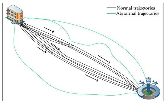
Figure 1.
Abnormal and normal trajectories.
- (1)
- Classification-based methods
The classification-based approach is a common supervised learning approach, which primarily includes logistic regression [14], decision trees [15], and support vector machines [16]. The classification-based abnormal-trajectory detection method detects abnormal behaviors in two stages. First, an abnormality-detection model is constructed by labeling the original data; then, the test data are input according to this model and is segregated into abnormal and normal categories.
Classification-based abnormal-trajectory detection methods can obtain more accurate results than unsupervised classification methods, but they require large, annotated datasets in advance. Trajectory paths are undirected and time varying, making it difficult to annotate all abnormal behaviors, and they do not apply to the detection of online streams.
- (2)
- Distance-based methods
Distance-based abnormality-detection methods primarily use distance functions (e.g., Euclidean, Manhattan, and dynamic time-warped distances) to calculate the distance between data objects [17]. San et al. [18] have proposed a method of scenario-aware distance-based outlier trajectory detection, which is divided into four main stages: feature extraction, distance matrix calculation, clustering, and outlier detection. The distance matrix between trajectories is calculated using a scenario-aware distance based on the results of feature extraction; group trajectories in homogeneous clusters are segmented and clustered, and the 1-nearest neighbor method is used to detect outliers in each cluster. Lee et al. [19] have proposed a segmentation and detection framework for trajectory-outlier detection that partitions the trajectory into a set of line segments and, subsequently, detects the abnormal line segments for trajectory outliers. They have also proposed the TRAOD algorithm, which first segments all trajectories and, then, detects the peripheral trajectory segments using a distance-based method. Yu et al. [20] have proposed “trajectory neighbors” to measure the similarity between different trajectories and designed a comprehensive strategy to efficiently detect outlier types in a large number of trajectory streams. They have proposed the minimum test (MEX) framework, which considers the spatial similarity between trajectory objects.
A distance-based algorithm focuses on the abnormality of location features, ignoring the role of other factors, and cannot accurately detect abnormalities caused by features other than the distance.
- (3)
- Historical similarity-based methods
Historical datasets were modeled based on the historical similarity method. Global features of the data were obtained from the data frequency, and trajectories with paradoxical features were identified based on the global features. Qian et al. [21] proposed an online abnormal cab trajectory detection method based on spatio-temporal relationships and defined two spatio-temporal models (D-S and D-T models) to describe the relationship between travel distance and time. The method retrieved the historical trajectory to calculate the displacement from the source to the test point, which was used to train the D-S and D-T models. The trajectory was identified as abnormal if the travel time and distance were not within the normal range of the model. Mao et al. [22] proposed a mechanism based on feature grouping, which introduced two isolated point definitions of local abnormal-trajectory fragments and evolutionary abnormal-motion objects. It calculated local abnormal-trajectory fragments and evolutionary abnormal-motion objects based on historical data, accumulated the product of all local abnormality factors of historical trajectory fragments, and generated a forward time-decay function [23]. They added the local abnormality factors of the current time-period trajectory fragments to obtain the evolutionary abnormality factor, which was used to obtain the evolutionary abnormal objects. Li et al. [24] proposed a method to detect temporal outliers using the aggregated time results of the entire dataset. They then calculated the similarity between road segments in each time period, recorded their historical similarity values in the temporal neighborhood vector of each road segment, and calculated the outliers based on the dramatic changes in the temporal neighborhood vector.
The abnormal-trajectory detection method based on historical trajectory similarity has high detection accuracy, but the trajectory data are time-varying. Therefore, it takes longer to reconstruct the model when the data changes incrementally.
- (4)
- Grid-based methods
The grid-based abnormality-detection method quantifies trajectories into a finite number of cells, converts each trajectory into a series of grid codes, and performs abnormality detection based on the grid codes. Zhang et al. [25] proposed an isolation-based abnormality-trajectory (iBAT) detection method. First, all cab trajectories passing through the same source–destination cell pair were grouped, and the cab trajectories were represented as an ordered sequence of symbols traversing the cells. Subsequently, iBAT was used to detect abnormal trajectories by applying an isolation mechanism to detect abnormal trajectories with the inherent property of “few and different”. Wang et al. [26] proposed a difference and intersection set distance metric to evaluate the similarity between two trajectories. They designed an abnormality scoring function to quantify the differences between different types of abnormal and normal trajectories, and further proposed an abnormal-trajectory detection and classification (ATDC) method to discover different abnormal trajectories. The trajectories were mapped into a two-dimensional grid space, converting the original trajectories into augmented trajectories consisting of a sequence of grid cells. This approach transforms the ATDC problem into a problem of finding and classifying abnormal trajectories from all trajectories with the same SD (fixed starting point S and fixed ending point D) pairs.
Most grid-based abnormal-trajectory detection methods use fixed grids, and the grid size affects the detection of abnormal trajectories. Abnormal trajectories may be mistakenly classified as normal trajectories if the grid size is set excessively large; conversely, normal trajectories may be classified as abnormal trajectories if the grid size is set excessively small.
- (5)
- Other methods
Yu et al. [27] proposed a new trajectory-outlier detection method based on a common slice subsequence in addition to the above abnormality-trajectory detection methods to address the problem of outlier trajectory detection in multiple consecutive abnormal segments. First, the direction code sequence of each trajectory segment was calculated. The sequence composed of trajectory slices was obtained by inflection point segmentation. The common slice sequence between two trajectories was used to measure their distance. Finally, the slice and trajectory outliers were detected based on the new common slice sequence distance. Wu et al. [28] proposed a multi-domain framework to study the spatio-temporal distribution of cab detour behavior at the directional road segment level. First, a map-matching-based detour clustering method was proposed to process the GPS data. A multi-layer road index system was then developed to account for the changes in the spatio-temporal distribution of cab detour characteristics and statistics, and a sample-based binary logit model was constructed. Zhao et al. [13] shifted the focus of abnormal-trajectory detection from trajectories to road networks. They constructed models from the perspective of road consumption (travel distance and time consumption) and implemented abnormal-trajectory detection using an unsupervised approach to obtain evaluation results closer to the actual situation.
The above abnormality-detection method does not consider the influence of road network density in determining abnormal trajectories, except for inherent defects. This ignores the relationship between the causes of abnormal-trajectory generation and road network density. The abnormal-trajectory detection method proposed in this study combines road network density and divides the urban region using variable grid sizes to improve the execution efficiency and accuracy rate of the algorithm.
The remainder of this paper is organized as follows. Section 2 presents the definitions, related statements, working framework, and algorithm description of the proposed method. The experimental evaluation and results are presented in Section 3. Section 4 discusses the contribution of the proposed method and presents the related analysis. Finally, Section 5 presents the conclusions and future research prospects.
2. Methods
2.1. Basic Concepts and Problem Description
This section defines the relevant concepts used in this study.
Definition 1 (Trajectory).
A trajectory is a sequence of GPS points during a taxi’s journey. The ith trajectory is denoted by = < , (), () …, () >, where denotes the trajectory identifier, and are the longitude and latitude of at , respectively (), and n denotes the number of points.
Definition 2 (SD-pair trajectories).
All trajectories with the same start place (S) and terminal place (D) are defined as SD-pair trajectories.
Definition 3 (Trajectory set).
The set formed by combining multiple SD pairs of trajectories is defined as a trajectory set and is represented by TD as follows:
where v denotes the number of trajectories in the trajectory set TD.
The subjects of this study were trajectories with fixed start and end places (i.e., SD-pair trajectories under specified start and end conditions).
Definition 4 (Trajectory tuple).
Let the trajectorypass through the high-, medium-, and low-density road network (road network) regions with grid codes,and; then, the trajectory tupleofis defined as follows:
Definition 5 (Number of grid codes).
The total number of cells that trajectorypasses through in each region is the number of grid codes, denoted as, as shown in Equation (3).
where,, anddenote the number of grids ofin the high-, medium-, and low-density regions, respectively.
Definition 6 (Standard trajectory).
Standard trajectory is defined as the trajectory with the least number of grid codes, and the set consisting of standard trajectories is called the standard trajectory set.
Definition 7 (Benchmark trajectory).
Let HT be the set of trajectories with the largest number of grids in the high-density road network region of the standard trajectory set; let MT be the set of trajectories with the largest number of grids in the medium-density road network region of HT. Any trajectory in MT is defined as the benchmark trajectory.
The trajectories in MT have the same number of grid codes in each type of density region as the standard trajectories have the same number of grid codes.
Definition 8 (Number of zone benchmark grids).
The number of grids in the benchmark trajectory set for any trajectory in the high-, medium-, and low-density regions is the zone benchmark grid number.
2.2. Variable-Grid-Based Abnormal-Trajectory Detection Method
The abnormality-detection based on variable grid (ATDVG) method proposed in this study includes three stages: road network density analysis, trajectory sequencing, and abnormal-trajectory detection. The road network density analysis and trajectory sequencing belong to the pre-processing stage before abnormal-trajectory detection. Figure 2 illustrates the working mode of the method.
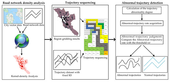
Figure 2.
Abnormality-detection framework.
Pre-processing stage: This stage includes road network density analysis and trajectory sequencing. First, the city region vector data and city road network data are input into ArcGIS, and the zoning results, which are divided into high-, medium-, and low-density road network regions, are obtained through kernel density analysis. Subsequently, the urban region with variable grid sizes is further divided. Finally, the fixed SD-pair trajectories are input into the gridded road network region to obtain the grid code of each trajectory.
Abnormal-trajectory detection stage: This stage consists of the following steps. Inputting the grid code to obtain the standard trajectory set, benchmarking the trajectory, and obtaining the number of zone benchmark grids. The trajectory abnormality degree of the remaining trajectory in each density region relative to the benchmark trajectory is determined, and the trajectory abnormality degree is compared with its corresponding number of zone benchmark grids. Finally, the trajectory abnormality value is calculated using the designed trajectory abnormality function and compared with the abnormality threshold rat to determine whether the trajectory is abnormal. A total of three algorithms are proposed in the abnormal-trajectory detection stage. Algorithm 1 obtains the number of zone benchmark grids. According to the number of zone benchmark grids, Algorithm 2 calculates the trajectory abnormality degree. Based on the trajectory abnormality degree, Algorithm 3 calculates the trajectory abnormality rate (TAR) and trajectory abnormality function value (TAP) for each trajectory and classifies the trajectories according to the abnormality threshold rat to obtain the abnormal trajectories.
2.2.1. Road Network Density Analysis
The city boundary vector and road network data were input into ArcGIS, and the kernel density analysis tool was used to delineate the road network density regions. As shown in Figure 3, in the density analysis, each route is covered with a surface, that is, the blue ellipse in Figure 3. Its density value is the largest at the location of the route and decreases gradually with the increase in the distance from the route. The density value is zero at the location where the distance from the route is equal to the specified search radius (blue curve). The density of a lattice element is equal to the sum of the densities superimposed on the center of the lattice element.
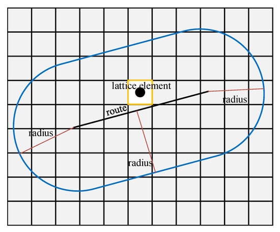
Figure 3.
Road network kernel density.
The kernel function used for road network analysis was adapted from the quadratic kernel function used to calculate the point densities described in previous studies [29] and to determine the default search radius, as shown in Equation (4).
where denotes the median distance from the mean center, DF denotes the standard deviation (calculated by the kernel density analysis tool), x represents the sum of all route values, and the min function represents the smaller DF and weighted used to calculate SearchRadius.
2.2.2. Trajectory Sequencing
The road network density is classified into three categories based on the results of the kernel density analysis via the natural-interruption-point grading method, which uses clustering to maximize the similarity within each class and dissimilarity between the outer classes, as follows: high, medium, and low. However, clustering does not focus on the number and range of elements in each class. The natural-interruption-point grading method also ensures that the range and number of densities between each class are as similar as possible. This shows that the high-density road network region is the smallest, the medium-density road network region is the second largest, and the low-density road network region is the largest. After dividing the area into three categories using the natural-interruption-point grading method (implemented using the function toolbox in ArcGIS), the regions with the higher and lowest density values are determined to be the high-density and low-density road network regions, and the remaining region is determined to be the medium-density road network region.
To improve the sensitivity of high-density road network regions to abnormality, as the detours mostly occur in high-density road network regions, this study sets the grid size relationship as: low-density road network region > medium-density road network region > high-density road network region. Fishnets were created for regions with different densities in ArcGIS. The grid sizes of the different regions were different, and the size of the fishnet was the grid size. Referring to previous studies [25,26], we set the initial size of the grid to 350 m × 350 m. In the experiments, after the trajectory visualization, we found that the detours occurred less in the medium-density road network region, and almost no detours occurred in the low-density road network region. According to the above situation, the region was divided to improve the sensitivity of the high-density road network region to abnormal trajectories. After gridding the different regions, a code is added to each grid in each region, and the fixed SD-pair trajectory set is input into ArcGIS. Each trajectory in conjunction with the regional grid codes is serialized, and the grid codes that each trajectory passes through in different regions are obtained as outputs and combined to form a trajectory tuple.
2.2.3. Abnormal-Trajectory Detection
- (1)
- Calculation of the trajectory abnormality degree
The benchmark trajectory set is removed from the trajectory set, and the difference in the remaining trajectory Ti, relative to the number of grid codes of the benchmark trajectory in each region, is defined as the trajectory abnormality degree, calculated as shown in Equations (5)–(7).
where , and are the numbers of zone benchmark grids in high-, medium-, and low-density regions, respectively; , , and denote the number of grids of in the high-, medium-, and low-density regions, respectively; and , , and denote the trajectory abnormality degrees of in the high-, medium-, and low-density road network regions, respectively.
The calculation of trajectory abnormality consists of two main steps: obtaining the number of zone benchmark grids, as shown in Algorithm 1, and calculating the trajectory abnormality based on the number of zone benchmark grids, as shown in Algorithm 2. Table 1 lists the relevant terms and symbols used in this algorithm.

Table 1.
Symbols used in the algorithm.
Initialization: Gn records the number of grids encoded for each trajectory in each density region; each row represents a trajectory. The first column records the identity of the corresponding trajectory; the second, third, and fourth columns record the number of grids for that trajectory in the high-, medium-, and low-density regions, respectively; the fifth column records the number of grids encoded for that trajectory.
| Algorithm 1: Zone benchmark grid number acquisition |
| Input: Original trajectory dataset TD, network coding number matrix Gn; Output: Number of zone datum grids , , ; matrix MT 1: NSG←min(Gn(:,5)); 2: k←0, q←0, r←0; 3: ST←, HT←, MT←; 4: for i←1 to |TD| 5: if Gn(i,5) == NSG 6: k←k + 1; 7: ST(k,:)←Gn(i,:); 8: end if 9: end for 10: ←max(ST(:,2)); 11: for i←1 to |ST| 12: if ST(i,2) == 13: q←q + 1; 14: HT(q,:)←ST(i,:); 15: end if 16: end for 17: ←max(HT(:,3)); 18: for i←1 to |HT| 19: if HT(i,3) == 20: r←r + 1; 21: MT(r,:)←HT(i,:); 22: end if 23: end for 24: ν←MT(1,4); 25: return , , , MT |
In Algorithm 1, Line 1 obtains the minimum value of the fifth column of the network coding number matrix Gn. Lines 2–3 initialize the relevant variables and matrices. Lines 4–9 obtain the standard trajectory set ST. Lines 10–16 obtain HT, which is the set of trajectories with the highest number of grids in the high-density road network region in the standard trajectory set. Lines 17–23 obtain MT, which is the set of trajectories with the highest number of grids in the medium-density road network region of HT. The time and space complexities of Algorithm 1 are O(q) and O(p), respectively, where q = n + |ST| + |HT| and p = |ST| + |HT| + |MT|.
| Algorithm 2: Trajectory abnormality degree calculation |
| Input: network coding number matrix Gn; matrix MT; Number of zone datum grids , , Output: The set of trajectory abnormality TP 1: TR←Gn-MT; 2: TP←; 3: for i←1 to |TR| 4: Calculate , , using Equations (5)–(7), respectively; 5: DAT←<, , >; 6: TP←TP DAT; 7: end for 8: return TP; |
In Algorithm 2, Line 1 removes the trajectories in the corresponding matrix MT from the network coding number matrix Gn. Line 2 initializes the matrix TP, which records the trajectory abnormality degree of the remaining trajectories. Lines 3–7 calculate the trajectory abnormality degree of the remaining trajectories after removing the matrix MT. The time and space complexities of Algorithm 2 are O(|TR|) and O(|TR|), respectively.
- (2)
- Abnormal-trajectory rate acquisition and abnormal judgment
The rate of the trajectory abnormality degree of each density region to the corresponding number of zone benchmark grids indicates the degree of abnormality of the trajectory relative to the benchmark trajectory. The degree of abnormality is expressed as the trajectory abnormality rate, which is calculated as shown in Equations (8)–(10).
where , and are the numbers of zone benchmark grids in high-, medium- and low-density regions, respectively; , , and denote the trajectory abnormality rates in high-, medium-, and low-density regions, respectively. According to Equations (8)–(10), we design and propose a TAP function, which is calculated as shown in Equation (11).
where , and the calculated result is compared with the abnormality threshold rat to determine whether is an abnormal trajectory.
The TAR acquisition and abnormality judgment are shown in Algorithm 3.
| Algorithm 3: Trajectory abnormality rate acquisition and abnormality judgment |
| Input: The set of abnormal trajectories TP; Trajectory abnormality threshold rat Output: Set of spatially abnormal trajectories TF 1: TF← ; 2: for i←1 to |TP| 3: Calculate , , and using Equations (8)–(10), respectively; 4: Calculate using Equation (11); 5: if 6: TF←TF TPi; 7: end if 8: end for 9: return TF; |
In Algorithm 3, Line 1 initializes the matrix TF. Lines 2–8 detect abnormal trajectories, where Lines 3–4 calculate TAR and TAP, respectively, and Lines 5–7 determine whether the trajectory is abnormal and classifies the trajectory. The time and space complexities of Algorithm 3 are O(|TP|) and O(|TF|), respectively.
2.2.4. Motivating Example
The detour behavior is mostly aimed at first-time visitors to the city, who generally arrive at the city center by train or high-speed rail (the red-boxed section), as shown in Figure 4. Long-distance visitors may go directly to some tourist attractions located in the low-density road network regions. The city center has a complex road network and high number of road options, while the low-density region, such as where tourist attractions are located, has fewer road options. Therefore, the urban region was only divided into high- and low-density regions, and this study assumed that the movement trajectory was from the high-density to the low-density region. In Figure 4, the high-density region is represented by the red box, and the rest represents the low-density region. The size of each grid in the high-density region is smaller than that in the low-density region, and g22 and g150 represent the starting and ending points of the trajectory, respectively.
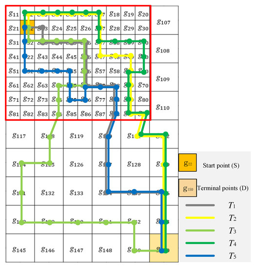
Figure 4.
Variable meshing of trajectories.
Supposing that there are five trajectories, denoted as , which are mapped in Figure 4, the resulting trajectory tuples are shown in Table 2.
Table 2.
The trajectory tuples of .
As indicated in Table 3, where NSG = 20, = 13, and = 7, the number of grids and grid codes corresponding to the high- and low-density road network regions in the example in Figure 4 are determined by Algorithm 2. As shown in Figure 4 and Table 3, the detours mostly occur in the high-density road network regions, and is the benchmark trajectory. The degree of abnormality of each trajectory was calculated separately according to , and the calculation results are listed in Table 4.
Table 3.
Number of grid codes for .
Table 4.
Calculation of DAT for .
Algorithm 3 was used to determine the TAR for each trajectory in the example in Figure 4; the findings are presented in Table 5.
Table 5.
Calculation of TAR for .
According to Equation (11), assuming (= 0), where = 0.6 and = 0.4, is used to indicate the sensitivity rate of the high-density road network region to abnormalities, and is used to indicate the sensitivity rate of the low-density road network region to abnormalities. According to Figure 4, we set to be greater than to improve the sensitivity rate of the high-density road network regions to abnormalities, as detour behavior is more likely to occur in the high-density road network regions. The results of the trajectory abnormalities of each trajectory were obtained, as shown in Table 6.
Table 6.
Calculation of TAP for .
The results in Table 6 show that if the trajectory is a normal trajectory, assuming rat = 0.2, is most likely to be an abnormal trajectory, followed by .
3. Results
The experiment was performed on a computer with an Intel Core i5 processor with a 3.10 GHz CPU. The operating platform was Windows 10, and the proposed algorithm was implemented using MATLAB 2020a. Accuracy, Precision, and Recall were used to measure the performance of the proposed abnormal-trajectory detection method and were calculated using Equations (12)–(14).
where TP denotes the actual number of true values in the sample predicted to be true, FP denotes the actual number of false values in the sample predicted to be true, FN denotes the actual number of true values in the sample predicted to be false, and TN denotes the actual number of false values in the sample predicted to be false.
3.1. Trajectory Dataset
This study used the dataset provided by Piorkowski et al. [30], containing trajectories of 536 cabs in the city of San Francisco, USA, over 30 days, with an average sampling rate of 100 s/point. The GPS trajectory data recorded the location (latitude and longitude) of each cab, as well as the corresponding time and occupancy. Only the trajectories between the San Francisco City Airport and central residential place were extracted.
3.2. Road Network Density Analysis
As shown in Figure 5a, the spatial distribution of the road networks in San Francisco is uneven, with the inner ring region having the highest road network density, followed by the inner and outer ring junction regions and outer ring region. In the kernel density analysis, the size of the lattice element should be smaller than the minimum grid size in the experiment. Referring to previous studies [25,26], the smallest grid size in our experiments was set as 350 m × 350 m. Combined with the kernel density analysis results, the lattice element size was set as 100 m × 100 m, and the city of San Francisco was divided into three regions, as shown in Figure 5b, where red indicates the denser region of the road network (grid image kernel density is 10.68–29.61), orange and yellow indicate the slightly dense region (grid image kernel density is 3.83–10.68) and the sparse region of the road network (grid image kernel density is 0–3.83), respectively.
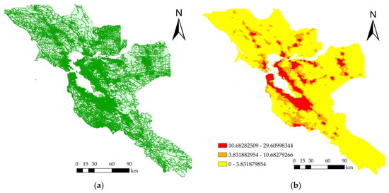
Figure 5.
Kernel density analysis: (a) San Francisco Bay region road network; (b) Results of kernel density analysis.
According to the results of the kernel density analysis, using the natural-interruption-point grading method, where different density regions are gridded, and the grid division size varies for different densities, the road network density is divided into three categories: high, medium, and low. Combined with the experimental analysis of ATDC [26] and iBAT [25], the grid sizes of the high-, medium-, and low-density road network regions were set as 350 m × 350 m, 500 m × 500 m, and 1 km × 1 km, respectively, as shown in Figure 6a. We extracted part of Figure 6a and enlarged it, as shown in Figure 6b. In the delineation process, the influence of the boundary of the remaining administrative district on trajectory abnormality determination can be ignored because of its small surface after gridding, as shown in the orange region.
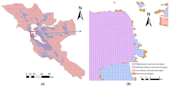
Figure 6.
Grid division results: (a) Grid division; (b) Extraction example.
3.3. Experimental Results
Four SD (residential region to the airport) pair (T-1 to T-4) trajectory sets were selected from 463,860 trajectories extracted from 1.12 million GPS points of 536 cabs to verify the performance of the proposed ATDVG method. The roads near residential places and the airport are more complex, and the roads between them are sparse, as shown in Figure 7. T-1, T-2, T-3, and T-4 contain 600, 301, 300, and 301 trajectories, respectively. We used the trajectories labeled in a previous study [26], as shown in Figure 1, where the trajectories marked in black are normal trajectories, and the trajectories marked in green are abnormal trajectories. The dataset and its labels are available at https://github.com/TUD-DD/ATDVG (assessed on 13 January 2023). T-1 was used as the training set and contained approximately the same number of normal and abnormal trajectories. T-2, T-3, and T-4 were used as the test sets. There are more normal trajectories of the same type in T-2, more normal trajectory types in T-4, and more normal trajectories than abnormal trajectories in T-2 and T-4. The T-3 dataset is the opposite of the T-2 dataset.
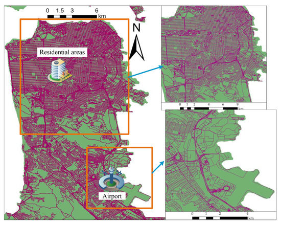
Figure 7.
Road network information.
The results of trajectory visualization on datasets T-1, T-2, T-3, and T-4 are shown in Figure 8a–d, respectively.
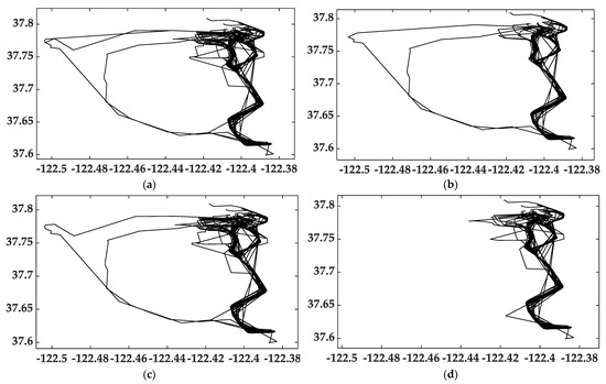
Figure 8.
Visualization of the original trajectories: (a) T-1; (b) T-2; (c) T-3; (d) T-4.
The detection results of ATDVG on datasets T-1, T-2, T-3, and T-4 are shown in Figure 9a–d, respectively.
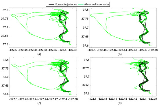
Figure 9.
Visualization of ATDVG results: (a) T-1; (b) T-2; (c) T-3; (d) T-4.
Figure 9 shows that ATDVG can detect most abnormal trajectories.
3.4. Varying Parameters
The parameters , , and are dynamically adjusted according to the different densities of road network regions through which the trajectory passes. According to Figure 7 and Figure 9, detours mainly occur in the high-density road network regions.
In this study, five parameters ( = , , ) were analyzed, where , as shown in Equation (15). The different parameter settings on the T-1 dataset were tested separately, and the highest values of Accuracy, Precision, and Recall were obtained for rat = 0.106 under each group of parameters. The experimental results of T-1, T-2, T-3, and T-4 under each group of parameter conditions are shown in Figure 10.
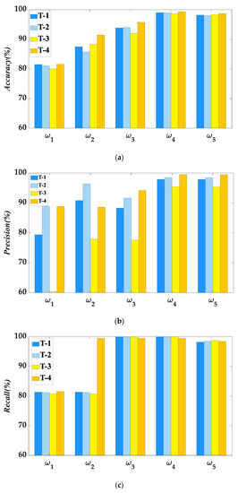
Figure 10.
Accuracy, Precision, and Recall values under different : (a) Different values of Accuracy values; (b) Different values of Precision values; (c) Different values of Recall values.
From Figure 10a–c, at = (0.70, 0.20, 0.10) and rat = 0.106, the proposed method can accurately determine the abnormal trajectory between the airport and the central residential region. Therefore, this study used the parameter and abnormality threshold rat = 0.106 for comparison with the fixed-grid method.
3.5. Comparative Evaluation
The ATDVG method was compared with the ATDC [26] and iBAT [25] methods to evaluate its performance in detecting abnormal trajectories. The iBAT method exploits the inherent property of “few and different” abnormal trajectories and applies an isolation mechanism to detect abnormal trajectories. ATDC is essentially a multi-classification problem that classifies trajectories into normal trajectories (NT), global detours (GD), local detours (LD), global shortcuts (GS), and local shortcuts (LS). In this study, NT, GS, and LS were considered normal trajectories, and GD and LD were considered abnormal trajectories. Table 7, Table 8 and Table 9 summarize the Accuracy, Precision, and Recall test results of the three methods (ATDVG, ATDC, and iBAT) for trajectory sets T-1, T-2, T-3, and T-4.
Table 7.
Accuracy comparison.
Table 8.
Precision comparison.
Table 9.
Recall comparison.
The detection results of ATDC on datasets T-1, T-2, T-3, and T-4 are shown in Figure 11a–d, respectively.
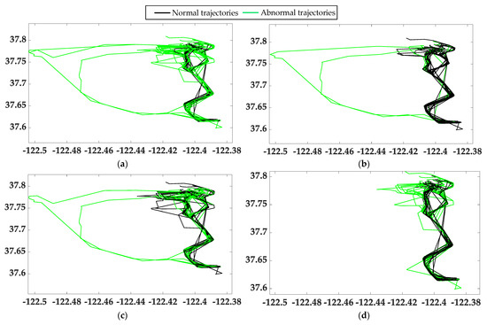
Figure 11.
Visualization of ATDC results: (a) T-1; (b) T-2; (c) T-3; (d) T-4.
The detection results of iBAT on datasets T-1, T-2, T-3, and T-4 are shown in Figure 12a–d, respectively.
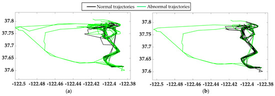
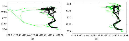
Figure 12.
Visualization of iBAT results: (a) T-1; (b) T-2; (c) T-3; (d) T-4.
Table 7, Table 8 and Table 9 summarize the Accuracy, Precision, and Recall test results of the three methods (ATDVG, ATDC, and iBAT) for trajectory sets T-1, T-2, T-3, and T-4. The proposed ATDVG method achieves the highest Accuracy, Precision, and Recall values on the four datasets. According to the visualization results, as shown in Figure 11 and Figure 12, ATDC and iBAT can detect the abnormal trajectories of a GD. The Accuracy, Precision, and Recall values of ATDC on T-2 are higher than those on T-1, T-3, and T-4, and the Accuracy value of iBAT on T-2 is higher than that on T-1, T-3, and T-4 because ATDC and iBAT usually detect abnormal trajectories according to the characteristics of “few and different”, and there are few spatial types of normal trajectories in T-2. Table 9 illustrates that the Recall value of iBAT is higher, and the Accuracy, Precision, and Recall values of ATDC on T-4 are smaller than those on T-1 and T-2 due to the large number of spatial types of normal trajectories in T-4. Some normal trajectories with a small number of spatial types may be judged as abnormal trajectories. The experimental results show that the Accuracy, Precision, and Recall values of ATDVG on T-4 are higher than those of ATDC and iBAT because ATDVG detects abnormal trajectories according to the “few and near” characteristics. Although there are more spatial types of normal trajectories in T-4, it has less influence on the ATDVG experimental results.
4. Discussion
The existing abnormal-trajectory detection methods usually require large amounts of trajectory data and a far greater number of normal trajectories than the number of abnormal trajectories. They also ignore the impact of the road network environment on abnormal-trajectory detection. Dividing the road network into fixed-size grids cannot reflect the difference in road network density in different regions; this is addressed by varying the grid sizes. The quadtree indexing method commonly used for trajectory simplification [31,32] can also generate grids of different sizes, but it is not suitable for research on complex road network environments. This study introduced the concept of a variable grid in conjunction with road network density and proposed the ATDVG method to solve these problems. First, the kernel density analysis was conducted in conjunction with the urban area and road network, dividing the city into three sub-regions based on the density of the urban road network, namely, high-, medium-, and low-density road network regions, each divided into grids of different sizes. Second, each source–destination trajectory was mapped to this two-dimensional grid space, and the grid codes of the different regions through which the trajectory passed were obtained. A trajectory tuple was used to integrate the grid codes to represent each trajectory, transforming the abnormal-trajectory detection problem into one of finding abnormal trajectories from grid codes with the same “source–destination pair.” Experiments with real trajectory datasets and road network data show that the proposed algorithm has higher matching accuracy and efficiency.
In real life, some detours may occur to save travel time. It is acceptable for some passengers to spend some extra money to arrive at their destination quickly. However, such detours are indeed abnormal in space, no matter the cause. This study only detects spatial anomalies, which may include such “positive” detours required by some passengers. For further time analysis, we calculated the shortest travel time of benchmark trajectories, which is used as the shortest travel time to compare with the travel time of the abnormal trajectories detected from each dataset. In the T-1 dataset, trajectories with less travel time than the shortest travel time account for only 0.0158 of the abnormal trajectories. In T-2, trajectories with less travel time than the shortest travel time account for only 0.0100 of the abnormal trajectories. In T-3, trajectories with less travel time than the shortest travel time account for only 0.0141 of the abnormal trajectories. In T-4, trajectories with less travel time than the shortest travel time account for only 0.0189 of the abnormal trajectories. According to these experimental results, time is saved by only a small part of the abnormal behaviors. Therefore, the spatial abnormality detection proposed in this paper is meaningful.
The main contributions of this study are as follows:
(1) A combination of road network and kernel density was applied for abnormal-trajectory detection, and the sensitivity of high-density road network regions to abnormality was improved by classifying different density regions based on the kernel density analysis results.
(2) The variable grid method was applied to the analysis of abnormal trajectories. The variable grid is used less in the field of abnormal-trajectory detection. This study combined grid division with the road network density to improve the accuracy of the grid abnormality-detection method.
(3) Trajectories are compared with the benchmark trajectory to prevent the rest of the trajectories in the domain with common subsegments from influencing the abnormality judgment for that trajectory.
The proposed algorithm improves the accuracy of abnormal-trajectory detection. The results of this study can help identify suspicious activities in vehicles and can be used in several applications, such as security monitoring and vehicle abnormality scheduling, to prevent taxi drivers from fraudulently adding trips to their customers for additional benefits.
5. Conclusions
Given the defect that the existing grid-based anomaly-detection methods do not consider the influence of road network density on trajectory anomaly detection, and only use grids with fixed sizes to divide regions, this study proposes an abnormal-trajectory detection method based on a variable grid, which compares each trajectory with the benchmark trajectory and analyzes them to prevent the influence of the remaining trajectories in the domain with common sub-fragments on the abnormal judgment of this trajectory. Additionally, the method uses the number of grids that the trajectory passes through to replace the travel distance and introduces variable grids in anomaly detection. Following kernel density analysis, the grid size varies for areas according to density. The grid size in high-density regions is smaller, which improves the difference between abnormal and normal trajectories. The grid size in low-density regions is larger, which improves the detection efficiency of abnormal trajectories. The method combines road network density analysis and uses variable grids to divide different regions, avoiding the poor anomaly detection problem caused by excessively large or small grid size.
However, the ATDVG method has some limitations. It cannot determine the specific segment of the abnormal trajectory that has problems, nor can it effectively determine the cause of the abnormality despite accurately determining the global abnormal trajectory. This is because of the complex causes of abnormal trajectories and lack of abnormal-trajectory data with annotations in the datasets used. In addition, the choice of benchmark trajectory determines the abnormality threshold, which requires trajectory datasets with high sampling frequencies. A higher number of grids in the high-density road network region improves the sensitivity of the region to abnormality. A slow trajectory may be judged as an abnormal trajectory if the trajectory dataset with a low sampling frequency is used because the parameter settings may improve the sensitivity of this type of region toward abnormality. Hence, the accuracy of this method in detecting low-sampling abnormal trajectories is low. Additionally, the location of the trajectory starting point for the ATDVG method is limited to the adjacent grid of the benchmark trajectory, which has high requirements for the starting point. Other features, such as length, time, direction, and speed, can be added in the future to further improve the accuracy of abnormal-trajectory detection.
Author Contributions
Conceptualization, Chuanming Chen; data curation, Dongsheng Xu; funding acquisition, Chuanming Chen, Qingying Yu and Wen Chen; methodology, Dongsheng Xu and Chuanming Chen; supervision, Chuanming Chen and Qingying Yu; validation, Shan Gong, Gege Shi and Haoming Liu; visualization, Chuanming Chen and Dongsheng Xu; writing—original draft, Dongsheng Xu; writing—review and editing, Qingying Yu, Shan Gong, Gege Shi and Haoming Liu. All authors have read and agreed to the published version of the manuscript.
Funding
This research was funded by the National Natural Science Foundation of China, grant numbers 61702010 and 61972439, the Anhui Provincial Natural Science Foundation of China, grant number 2208085MF164, the University Natural Science Research Program of Anhui Province, grant number KJ2021A0125, and the Major Natural Science Research Projects of Higher Education Institutions in Anhui Province, grant number KJ2020ZD61.
Institutional Review Board Statement
Not applicable.
Informed Consent Statement
Not applicable.
Acknowledgments
The authors would like to thank the reviewers for their useful comments and suggestions for this paper.
Conflicts of Interest
The authors declare no conflict of interest.
References
- Ranaweera, M.; Seneviratne, A.; Rey, D.; Saberi, M.; Dixit, V.V. Detection of anomalous vehicles using physics of traffic. Veh. Commun. 2021, 27, 100304. [Google Scholar] [CrossRef]
- Xia, F.; Wang, J.; Kong, X.; Wang, Z.; Li, J.; Liu, C. Exploring human mobility patterns in urban scenarios: A trajectory data perspective. IEEE Commun. Mag. 2018, 56, 142–149. [Google Scholar] [CrossRef]
- Qiao, Y.; Cheng, Y.; Yang, J.; Liu, J.; Kato, N. A mobility analytical framework for big mobile data in densely populated area. IEEE Trans. Veh. Technol. 2017, 66, 1443–1455. [Google Scholar] [CrossRef]
- Wang, Y.; Zheng, Y.; Xue, Y. Travel time estimation of a path using sparse trajectories. In Proceedings of the ACM SIGKDD International Conference on Knowledge Discovery and Data Mining, New York, NY, USA, 24–27 August 2014; pp. 25–34. [Google Scholar]
- Chiabaut, N.; Faitout, R. Traffic congestion and travel time prediction based on historical congestion maps and identification of consensual days. Transp. Res. Part C Emerg. Technol. 2021, 124, 102920. [Google Scholar] [CrossRef]
- Ning, Z.; Huang, J.; Wang, X. Vehicular fog computing: Enabling real-time traffic management for smart cities. IEEE Wirel. Commun. 2019, 26, 87–93. [Google Scholar] [CrossRef]
- Ding, Y.; Zhang, W.; Zhou, X.; Liao, Q.; Luo, Q.; Ni, L.M. FraudTrip: Taxi fraudulent trip detection from corresponding trajectories. IEEE Internet Things J. 2021, 8, 12505–12517. [Google Scholar] [CrossRef]
- Lu, E.H.-C.; Chen, H.S.; Tseng, V.S. An efficient framework for multirequest route planning in urban environments. IEEE Trans. Intell. Transp. Syst. 2017, 18, 869–879. [Google Scholar] [CrossRef]
- Tu, W. Real-Time route recommendations for E-Taxies leveraging GPS trajectories. IEEE Trans. Ind. Inform. 2021, 17, 3133–3142. [Google Scholar] [CrossRef]
- Gao, Q.; Zhang, F.L.; Wang, R.J.; Zhou, F. Trajectory big data: A review of key technologies in data processing. Ruan Jian Xue Bao/J. Softw. 2017, 28, 959–992. [Google Scholar]
- Wang, Y.; Qin, K.; Chen, Y.; Zhao, P. Detecting anomalous trajectories and behavior patterns using hierarchical clustering from Taxi GPS Data. ISPRS Int. J. Geo-Inf. 2018, 7, 25. [Google Scholar] [CrossRef]
- Qin, G.; Huang, Z.; Xiang, Y.; Sun, J. ProbDetect: A choice probability-based taxi trip anomaly detection model considering traffic variability. Transp. Res. Part C Emerg. Technol. 2019, 98, 221–238. [Google Scholar] [CrossRef]
- Zhao, X.; Su, J.; Cai, J.; Yang, H.; Xi, T. Vehicle anomalous trajectory detection algorithm based on road network partition. Appl. Intell. 2022, 52, 8820–8838. [Google Scholar] [CrossRef]
- Tao, L.; Zhu, D.; Yan, L.; Zhang, P. The traffic accident hotspot prediction: Based on the logistic regression method. In Proceedings of the ICTIS 2015—3rd International Conference on Transportation Information and Safety, Wuhan, China, 25–28 June 2015; pp. 107–110. [Google Scholar]
- Kim, T.; Taylor, S.; Yue, Y.; Matthews, I. A decision tree framework for spatiotemporal sequence prediction. In Proceedings of the ACM SIGKDD International Conference on Knowledge Discovery and Data Mining, Sydney, Australia, 10–13 August 2015; pp. 577–586. [Google Scholar]
- Piciarelli, C.; Micheloni, C.; Foresti, G.L. Trajectory-based anomalous event detection. IEEE Trans. Circuits Syst. Video Technol. 2008, 18, 1544–1554. [Google Scholar] [CrossRef]
- Knorr, E.M.; Ng, R.T.; Tucakov, V. Distance-based outliers: Algorithms and applications. VLDB J. 2000, 8, 237–253. [Google Scholar] [CrossRef]
- San Román, I.; de Diego, I.M.; Conde, C.; Cabello, E. Outlier trajectory detection through a context-aware distance. Pattern Anal. Appl. 2019, 22, 831–839. [Google Scholar] [CrossRef]
- Lee, J.G.; Han, J.; Li, X. Trajectory outlier detection: A partition-and-detect framework. In Proceedings of the International Conference on Data Engineering, Urbana, IL, USA, 7–12 April 2008; pp. 140–149. [Google Scholar]
- Yu, Y.; Cao, L.; Rundensteiner, E.A.; Wang, Q. Detecting moving object outliers in massive-scale trajectory streams. In Proceedings of the ACM SIGKDD International Conference on Knowledge Discovery and Data Mining, New York, NY, USA, 24–27 August 2014; pp. 422–431. [Google Scholar]
- Qian, S.; Cheng, B.; Cao, J.; Xue, G.; Zhu, Y.; Yu, J.; Li, M.; Zhang, T. Detecting taxi trajectory anomaly based on spatio-temporal relations. Intell. Transp. Syst. 2022, 23, 6883–6894. [Google Scholar] [CrossRef]
- Mao, J.; Wang, T.; Jin, C.; Zhou, A. Feature grouping-based outlier detection upon streaming trajectories. IEEE Trans. Knowl. Data Eng. 2017, 29, 2696–2709. [Google Scholar] [CrossRef]
- Cormode, G.; Shkapenyuk, V.; Srivastava, D.; Xu, B. Forward decay: A practical time decay model for streaming systems. In Proceedings of the International Conference on Data Engineering, Las Vegas, NV, USA, 22–24 June 2009; pp. 138–149. [Google Scholar]
- Li, X.; Li, Z.; Han, J.; Lee, J.G. Temporal outlier detection in vehicle traffic data. In Proceedings of the International Conference on Data Engineering, Shanghai, China, 29 March–2 April 2009; pp. 1319–1322. [Google Scholar]
- Zhang, D.; Li, N.; Zhou, Z.H.; Chen, C.; Sun, L.; Li, S. iBAT: Detecting anomalous taxi trajectories from GPS traces. In UbiComp’11, Proceedings of the 2011 ACM Conference on Ubiquitous Computing, Beijing, China, 17–21 September 2011; Association for Computing Machinery: New York, NY, USA, 2011; pp. 99–108. [Google Scholar]
- Wang, J.; Yuan, Y.; Ni, T.; Ma, Y.; Liu, M.; Xu, G.; Shen, W. Anomalous trajectory detection and classification based on difference and intersection set distance. IEEE Trans. Veh. Technol. 2020, 69, 2487–2500. [Google Scholar] [CrossRef]
- Yu, Q.; Luo, Y.; Chen, C.; Wang, X. Trajectory outlier detection approach based on common slices sub-sequence. Appl. Intell. 2018, 48, 2661–2680. [Google Scholar] [CrossRef]
- Wu, Z.; Li, Y.; Wang, X.; Su, J.; Yang, L.; Nie, Y.; Wang, Y. Mining factors affecting taxi detour behavior from GPS traces at directional road segment Level. IEEE Trans. Intell. Transp. Syst. 2022, 23, 8013–8023. [Google Scholar] [CrossRef]
- Silverman, B.W. Density estimation for statistics and data analysis. Wiley R. Stat. Soc. 2016, 150, 403–404. [Google Scholar]
- Piorkowski, M.; Sarafijanovic-Djukic, N.; Grossglauser, M. CRAWDAD. (v. 2009-02-24). Available online: https://crawdad.org/epfl/mobility/20090224 (accessed on 1 March 2021).
- Fu, C.; Huang, H.; Weibel, R. Adaptive simplification of GPS trajectories with geographic context–a quadtree-based approach. Int. J. Geogr. Inf. Sci. 2021, 35, 661–688. [Google Scholar] [CrossRef]
- Lee, W.; Cho, S.W. AIS Trajectories Simplification Algorithm Considering Topographic Information. Sensors 2022, 22, 7036. [Google Scholar] [CrossRef] [PubMed]


Disclaimer/Publisher’s Note: The statements, opinions and data contained in all publications are solely those of the individual author(s) and contributor(s) and not of MDPI and/or the editor(s). MDPI and/or the editor(s) disclaim responsibility for any injury to people or property resulting from any ideas, methods, instructions or products referred to in the content. |
© 2023 by the authors. Licensee MDPI, Basel, Switzerland. This article is an open access article distributed under the terms and conditions of the Creative Commons Attribution (CC BY) license (https://creativecommons.org/licenses/by/4.0/).