Abstract
To promote the development of deep learning for feature matching, image registration, and three-dimensional reconstruction, we propose a method of constructing a deep learning benchmark dataset for affine-invariant feature matching. Existing images often have large viewpoint differences and areas with weak texture, which may cause difficulties for image matching, with respect to few matches, uneven distribution, and single matching texture. To solve this problem, we designed an algorithm for the automatic production of a benchmark dataset for affine-invariant feature matching. It combined two complementary algorithms, ASIFT (Affine-SIFT) and LoFTR (Local Feature Transformer), to significantly increase the types of matching patches and the number of matching features and generate quasi-dense matches. Optimized matches with uniform spatial distribution were obtained by the hybrid constraints of the neighborhood distance threshold and maximum information entropy. We applied this algorithm to the automatic construction of a dataset containing 20,000 images: 10,000 ground-based close-range images, 6000 satellite images, and 4000 aerial images. Each image had a resolution of 1024 × 1024 pixels and was composed of 128 pairs of corresponding patches, each with 64 × 64 pixels. Finally, we trained and tested the affine-invariant deep learning model, AffNet, separately on our dataset and the Brown dataset. The experimental results showed that the AffNet trained on our dataset had advantages, with respect to the number of matching points, match correct rate, and matching spatial distribution on stereo images with large viewpoint differences and weak texture. The results verified the effectiveness of the proposed algorithm and the superiority of our dataset. In the future, our dataset will continue to expand, and it is intended to become the most widely used benchmark dataset internationally for the deep learning of wide-baseline image matching.
1. Introduction
In recent years, because of advances in technologies such as ground-moving wide-baseline photography, unmanned aerial vehicle (UAV) oblique photography, and cross-directional observation by multiple satellites, the large number of images produced (in the form of big data) cover the sky and the earth. Stereo images formed by these new data have large differences in viewpoint. Therefore, the scale, orientation, surface brightness, and neighborhood information of the same spatial target in the stereo images may be missing or distorted in a complex manner. This poses a severe challenge to image matching. Deep learning, a data-driven method for high-level feature representation based on a neural network architecture, has been applied in the field of image matching [1]. However, at the present time, existing affine-invariant deep learning models still have difficulty matching stereo images with large viewpoint differences [2]. One reason for this problem is that existing, publicly available benchmark datasets for affine-invariant feature matching are small in scale and contain only a single texture type; the other reason is that existing methods for constructing affine-invariant feature-matching datasets often rely on the manual measurement of the corresponding features [3,4,5,6].
The training samples for affine-invariant feature matching contained in the Brown dataset [7] are derived from ground-based, close-range images that are dominated by artificial statues and natural landscapes. Most of the corresponding patches in the Brown dataset were manually selected; this manual selection may be time-consuming and laborious. In addition, it is limited by the scale and breadth of the dataset. Consequently, the trained model is not sufficiently generalizable to wide-baseline images captured from aerial or satellite platforms. The key to the production of training datasets for image matching is the quantity and quality of the corresponding features extracted. Handcrafted methods, represented by the scale-invariant feature transform (SIFT) [8] algorithm, employ a three-step strategy to automatically extract the corresponding features. First, scale-invariant features are detected, then the gradient descriptors are generated, and finally, matches are obtained using the nearest/next distance ratio (NNDR) metric and the random sampling consensus (RANSAC) strategy [9]. The SIFT algorithm cannot adapt to affine-distorted images with large viewpoint differences, although it has good scale invariance. Yang et al. [10] first used SIFT to obtain the initial matches and then used the normalized cross-correlation strategy with affine correction to generate more matches. Zhang et al. [11] extracted the feature points within the normalized regions using filter decomposition and phase consistency and used the Gaussian mixture model to determine the transformation matrix across the corresponding points of the stereo images, thereby improving the positioning accuracy of features within the affine-invariant regions. Xiao et al. proposed an affine-invariant method for oblique image matching. This calculates the initial affine matrix from the image orientation parameters, then corrects the oblique image according to the affine matrix, and finally applies the SIFT algorithm to the corrected images to perform oblique image matching [12,13]. Jiang et al. used external orientation elements to perform a global geometric correction of oblique images and then applied the SIFT algorithm to perform extraction and matching of image features; however, the practicability of this method is very limited because it requires known camera pose parameters [14]. Affine-SIFT (ASIFT) [15] first simulates the attitude angles of photography in three-dimensional space; it then generates numerous rectified image sequences by projection transformation; finally, it applies the SIFT algorithm to extract the corresponding features from these simulated images. This method has good affine invariance, but it has difficulty obtaining the corresponding features from image regions with poor texture.
Deep learning algorithms, based on convolutional neural networks (CNNs), constitute new methods for affine-invariant feature matching [16]. Compared with handcrafted methods, designers of deep learning algorithms for image matching do not need to artificially design an intuitive calculation model and its empirical parameters; instead, they need to construct a CNN and its loss function. The CNN iteratively learns the optimal convolutional representation of target features from a large number of matching labels. Current deep learning methods for image matching are divided into dense matching and sparse matching methods. The former methods directly compute the pixel-by-pixel dense correspondence of overlapping regions by estimating a stereo disparity map; the latter methods perform stage-wise training and optimization on feature extraction, description, and correlation and demonstrate better matching reliability in practice [17]. The most typical representative of sparse matching methods is L2-Net [18], which trains the Euclidean distance between matching descriptors as closely as possible using loop iterations of a Siamese network. HardNet [19] is based on L2-Net but adds the distance learning of non-matching descriptors to significantly improve the discrimination between descriptors. Mishkin et al. employed the multi-scale Hessian operator to detect initial feature points and estimated the affine-invariant neighborhood using the triplet network, AffNet [20]. This method combines traditional feature detection with deep learning invariant regions and significantly improves the efficiency and reliability of feature extraction. Inspired by the SuperGlue [21] model, Sun et al. introduced the position encoding and attention mechanism in the transformer [22] network and constructed a model named the local feature transformer (LoFTR) [23] with a texture enhancement function; this method significantly improves the matching performance in regions with weak texture.
In summary, the main existing problems can be listed as follows: (1) It lacks an efficient automatic production method for affine-invariant feature-matching deep learning datasets; (2) the existing datasets are too homogeneous in terms of data types; and (3) the existing evaluation criteria for the spatial distribution of the matches are not precise enough.
The ASIFT algorithm is adaptable to wide-baseline oblique images, which often have large affine distortions, and the LoFTR method can extract the corresponding features from regions with weak texture. Therefore, the complementary fusion of the two methods can effectively obtain more corresponding features distributed across regions of different types. The number of panoramic images released by Baidu Maps has already exceeded 2 billion, and they cover more than 95% of the urban street scenes in China. In addition, the open-source satellite images of Google Maps cover more than 95% of the world, with a maximum resolution of 0.25 m. These open-source images provide an extensive source of image data for the production of a benchmark dataset. For this reason, this paper proposes a novel method for constructing a benchmark dataset for deep learning. First, the complementary ASIFT and LoFTR algorithms are integrated to significantly increase the types of matching regions and the number of corresponding features. Next, matching points with uniform spatial distributions are selected according to the hybrid constraint of the neighborhood distance threshold and maximum information entropy, and then a high-quality matching benchmark is produced. Using our algorithm, a rich affine-invariant deep learning benchmark dataset, named SJRS, is automatically constructed. This dataset is intended to promote the application of deep learning to intelligent image matching.
Differing from HPatches [24] and MegaDepth [25] datasets, our dataset (SJRS) consists of 1024 × 1024 bitmap (.bmp) images, each of which contain an array of 16 × 16 image patches, and each patch is sampled as a 64 × 64 grey scale with a normalized region and orientation. SJRS is of a similar type to the Brown dataset [7], but it contains more image types from ground-based close-range, aerial, and satellite platforms and is larger in scale than Brown. The contributions of this paper are as follows.
- An effective algorithm for the production of a deep learning dataset for affine-invariant feature matching.
- The most extensive deep learning benchmark dataset to date for affine-invariant feature matching.
- A distribution evaluation model that considers both global and local image contents to accurately evaluate the spatial distribution quality for matching points.
2. Data and Methods
Figure 1 shows the strategy for the automatic construction of a dataset for affine-invariant feature matching. The key steps of this method are as follows. First, the complementary algorithms, ASIFT [15] and LoFTR [23], are integrated to extract quasi-dense corresponding features across wide-baseline oblique stereo images (Yellow part of Figure 1). Second, spatially uniform corresponding features are selected from the quasi-dense matches (Orangered part of Figure 1). Third, the stitching dataset is generated from the generated corresponding patches with various texture types (Light blue part of Figure 1). The method is rigorous, easy to implement, and can be executed in parallel. This section describes the main method, including the dataset of wide-baseline oblique images, extraction of quasi-dense complementary corresponding features, optimization for uniform matches, and automatic stitching of the dataset.
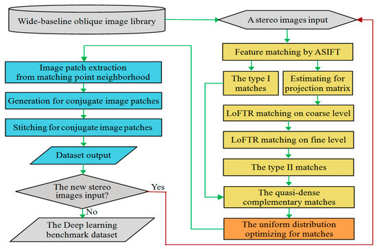
Figure 1.
Flowchart for the automatic production of an affine-invariant feature-matching dataset.
2.1. Wide-Baseline Oblique Image Library
We collected 8668 pairs of wide-baseline oblique stereo images from various photography platforms: a ground-based mobile survey vehicle, an aircraft, and a satellite.
The ground-based close-range images (3879 pairs) and satellite images (3000 pairs) were obtained from Baidu and Google Maps, respectively, and aerial images (1789 pairs) were freely provided by the China Academy of Surveying and Mapping. The ground-based close-range images mostly covered various outdoor scenes, such as building walls, cement roads, dirt roads, trees, hillsides, ponds, ditches, and sandy land; the aerial images mostly covered the tops and sides of buildings, woodlands, grasslands, cultivated lands, ports, docks, lakes, rivers, wastelands, and other surface scenes of small areas; the satellite images mostly covered large-scale surface scenes, such as urban areas, suburbs, snowfields, grasslands, forests, and mountainous areas. There were notable differences in field depth, local occlusion, and grayscale between the ground-based close-range and aerial stereo images, and radiation distortion and local object differences appeared in the satellite stereo images; in addition, all stereo images had significant viewpoint differences. Figure 2 shows some randomly selected images from the dataset.
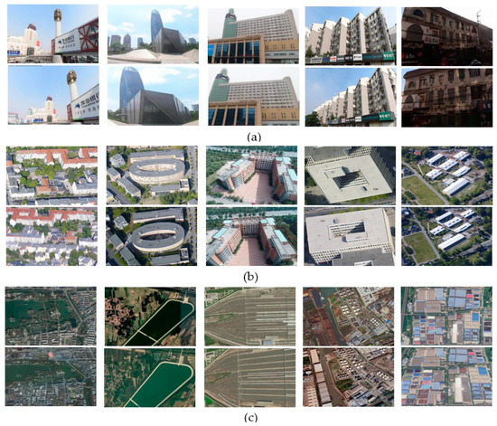
Figure 2.
Thumbnail of partial, wide-baseline oblique stereo images from ground close-range (a), airborne (b), and space platforms (c).
2.2. Extraction of Quasi-Dense Conjugate Points Using Complementary Features
The strategy for complementary feature extraction for quasi-dense matches is illustrated in Figure 3, in which the red and green points represent the type-I (ASIFT) and type-II (LoFTR) matches, respectively. The figure shows that they have good complementarity. The method of extracting the two types of features is briefly described below.
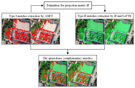
Figure 3.
Illustration of quasi-dense matching using complementary features. The type-I (ASIFT) and type-II (LoFTR) matches are represented by red and green points, respectively.
The extraction of type-I matches was based on ASIFT [15]. First, the scale variation, rotation difference, and viewpoint difference between stereo images were simulated and resampled. Second, the simulated stereo image sequences were matched by SIFT. Third, coordinate transformation was performed for the corresponding features in each simulated image, and then the corresponding points were output in the original image coordinate system. For wide-baseline oblique stereo images from the aerial, satellite, and ground-based close-range platforms, the ASIFT algorithm was applied to obtain a large number of corresponding features (named type-I features). Most of these features were distributed across regions with rich texture information. However, ASIFT had difficulty recognizing features in regions with poor or weak texture.
The extraction of type-II matches was performed by LoFTR [23] with projection transformation. The LoFTR method could effectively extract the corresponding features from regions with weak texture, but it was sensitive to affine deformation between images; therefore, it was difficult to apply it directly to wide-baseline oblique image matching. For this purpose, the RANSAC algorithm was first used to estimate the projection transformation matrix H from the type-I matches using Equation (1).
where (x, y) and (x′, y′) denote the type-I matching points in the left and right images, respectively, and are the nine projection coefficients in matrix H. The right image can then be corrected by
where (x′, y′) and (x″, y″) denote the pixel coordinates before and after the geometric correction of the right image, respectively. After the right image was corrected by projection transformation, the affine distortion of the corresponding regions was greatly reduced. The LoFTR method with this transformation was used for image matching. The LoFTR algorithm, illustrated in Figure 4, contains four key steps, as follows.
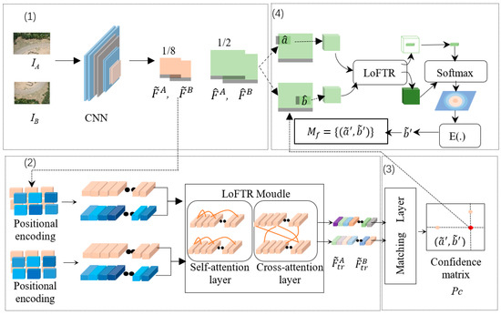
Figure 4.
Architecture of the local feature transformer (LoFTR) model.
- (1)
- One image pair, IA and IB, was input into the CNN for feature extraction. The coarse (1/8) feature maps of the two images were denoted by and , respectively, and the fine (1/2) feature maps were denoted by and , respectively.
- (2)
- and were flattened to one-dimensional vectors, and positional encodings were produced for them. The vectors with positional encoding were then processed by the LoFTR module, which had two self-attention layers and two cross-attention layers. Finally, two texture- and feature-enhanced maps, and , with high discrimination, were output.
- (3)
- The differential matching layer was used to match the high-discrimination feature maps, and , to obtain a confidence matrix Pc. The matches in Pc were then determined according to the confidence threshold (0.2 in our experiment) and the mutual nearest neighbor criterion, and the coarse-level matching prediction Mc was obtained.
- (4)
- For each coarse-level matching prediction (i, j) in Mc, local corresponding windows with a size of 5 × 5 pixels were captured around and . Similarly, all coarse matches were refined according to fine-level local windows, and then the final sub-pixel matching prediction Mf was output.
It should be noted that all the matching points in the right image needed to be converted to the original image coordinate system by Equation (2) to obtain the type-II matching features. The type-I and type-II matches were then combined, and the quasi-dense complementary matching points were output.
2.3. Generation of Uniform Matching Points
The quasi-dense corresponding features obtained, as explained in the previous section, had good spatial complementarity, but there were also many adjacent, dense matches. Capturing the corresponding patches would inevitably generate many duplicate datasets, thereby reducing the performance of the datasets and the training efficiency of the model. Therefore, the quasi-dense matches needed to be optimized by sparsification. Figure 5 shows the optimization strategy for generating uniform matching points by hybrid constraints: the matching point statistics were calculated for every s-pixel (s = 32 in our experiment) neighborhood, and the information entropy was calculated for each matching point in the neighborhood according to the following equation:
where m denotes the number of gray values in the r-pixel (r = 7 in our experiment) neighborhood of the current matching point, and Pj is the probability of the j-th gray value in the neighborhood appearing in the whole image; the matching point with the highest information entropy in the s-pixel neighborhood was retained. All matching neighborhoods of the stereo images were processed similarly to perform matching optimization. The red and green points in Figure 5 represent the type-I and type-II matching points, respectively. It can be observed that the results of sparse optimization had good spatial complementarity and a uniform distribution. These results provided the foundation for the subsequent generation of a high-quality dataset.
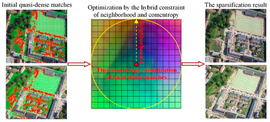
Figure 5.
Illustration of the optimal selection of uniform matching points.
2.4. Automatic Production of Dataset
The algorithm for automatically generating a dataset is illustrated in Figure 6. First, image patches with a size of 64 × 64 pixels were extracted from the corresponding neighborhoods, which were centered at matching points, and numerous corresponding patches were generated. Second, a blank image with a size of 1024 × 1024 pixels was constructed, and the corresponding patches were placed in the blank image in sequence by column and row. In this image, each row included eight pairs of corresponding patches, resulting in 16 image blocks in each row and column. This process was repeated for each image in the dataset. Finally, the number of channels and file name of each dataset image was sequentially formatted and converted to the normal form required by the target deep learning network. By executing this process in parallel, we efficiently constructed the SJRS dataset with 20,000 images: 10,000 ground-based close-range images, 6000 satellite images, and 4000 aerial images from UAVs. It is publicly available at https://github.com/Zhangjin0357/SJRS (accessed on 5 July 2022).
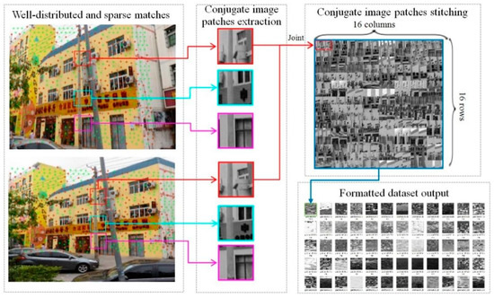
Figure 6.
Algorithm for the automatic production of the dataset.
3. Results and Discussion
3.1. Model Training
The experimental environment was a computer with an NVIDIA GeForce RTX 2080 Ti GPU, Intel Core i99-9900K CPU, 64 GB memory, and the Ubuntu 18.04 operating system. The AffNet network was reconstructed using the Python programming language and the PyTorch framework. The AffNet model was trained on the Brown dataset [7] and our SJRS dataset, and the trained models were named Brown-AffNet and SJRS-AffNet, respectively. The training parameters were uniformly set as follows. The batch size was 1024, the number of iterations was 30, the learning rate was 0.005, the momentum hyperparameter was 0.9, the weight decay value was 0.0001, and the stochastic gradient descent was used as the optimizer.
3.2. Test Methods
To verify the superiority of the SJRS dataset and the trained model proposed in this paper, three methods were used to perform affine-invariant feature extraction: (1) ASIFT; (2) Brown-AffNet; and (3) SJRS-AffNet. Methods (2) and (3) employed HardNet to generate feature descriptors with 128 dimensions and obtained feature matches using the NNDR metric (with the threshold set to 0.8). They all adopted the RANSAC algorithm to eliminate possible outliers. To objectively evaluate the matching performance of the three methods, nine pairs of wide-baseline oblique images (shown in Figure 7) were selected as representative test data; each pair of images had significant geometric and radiation distortions. There were three sets of image pairs: JJ1–3 were ground-based close-range images, covering areas with little texture, such as walls, ground, and glass surfaces, and containing some regions that had parallax discontinuity; HK1–3 were aerial images, covering areas lacking texture, such as bare ground, stadiums, and residential areas, and containing terrain undulations in local areas; WX1–3 were satellite images, covering areas with little texture, such as suburbs, parks, and airports, and including the difference of ground objects between images.
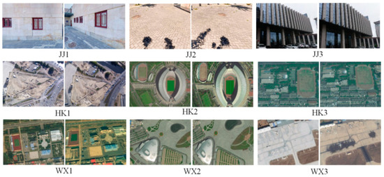
Figure 7.
Thumbnails of test data images.
3.3. Evaluation Metrics
- (1)
- Number of correct matching points . Fifteen pairs of uniformly distributed corresponding points were manually selected from stereo image pairs, the fundamental matrix F0 was estimated by least-squares adjustment, and this was regarded as the ground truth [26,27,28]. The known fundamental matrix, F0, was used to calculate the error of each matching point according to Equation (4), and a threshold, (set to 2.0), was imposed for the error. If the error was less than , the pair of points was a correct pair of matching points and was included in the count of correct matching points .where and denote any pair of corresponding points.
- (2)
- Match correct rate α. This was defined by α = , where k denotes the total number of matching points.
- (3)
- Matching root-mean-square error (pixel). This was calculated according to the following equation:
- (4)
- Matching spatial distribution quality . Zhu et al. generated a Delaunay triangulation [29] from the matching points and then evaluated the quality of the spatial distribution of the matching points according to the area and shape of each triangle, as shown in Equation (6):
3.4. Results and Analysis
Figure 8 shows the matching results of the three methods on the ground-based close-range stereo images JJ1–3. Figure 9 shows the results of the methods trained on the aerial stereo images HK1–3. Figure 10 shows the results of the methods trained on the satellite stereo images WX1–3. The green points in the figures represent the final matching results of each method. To clearly compare the matching performances of the methods, the matching results of some local areas of each image were selected with red boxes and displayed at an enlarged scale. In addition, to determine the matching distribution quality of the methods, a Delaunay triangulation was automatically generated from the matching results of each method, as shown in Figure 11, Figure 12 and Figure 13. Finally, Table 1 presents the quantitative experimental results of the three methods tested on the aerial, satellite, and ground-based close-range test data. Here, and α denote the number of correct matching points and match correct rate, respectively, and and denote the match correct rate and matching spatial distribution quality, respectively. The best value of the metric for each group of data in the table is highlighted in bold.
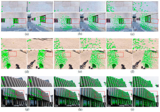
Figure 8.
Matching results of the three methods tested on ground-based close-range stereo images JJ1–3. (a,d,g) tested on ASIFT. (b,e,h) tested on Brown-AffNet. (c,f,i) tested on SJRS-AffNet.
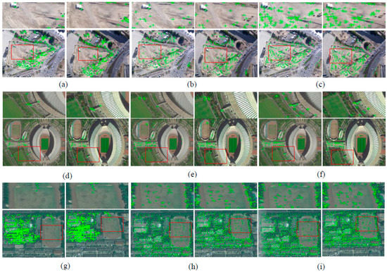
Figure 9.
Matching results of the three methods tested on aerial stereo images HK1–3. (a,d,g) tested on ASIFT. (b,e,h) tested on Brown-AffNet. (c,f,i) tested on SJRS-AffNet.
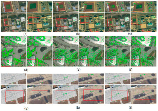
Figure 10.
Matching results of the three methods tested on satellite stereo images WX1–3. (a,d,g) tested on ASIFT. (b,e,h) tested on Brown-AffNet. (c,f,i) tested on SJRS-AffNet.
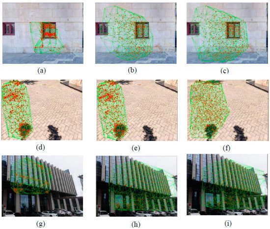
Figure 11.
Delaunay triangulation network of matches from ground-based close-range stereo images JJ1–3. (a,d,g) tested on ASIFT. (b,e,h) tested on Brown-AffNet. (c,f,i) tested on SJRS-AffNet.
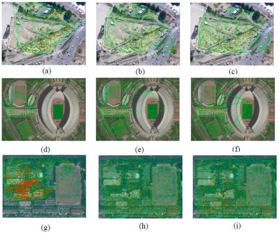
Figure 12.
Delaunay triangulation network of matches from aerial stereo images HK1–3. (a,d,g) tested on ASIFT. (b,e,h) tested on Brown-AffNet. (c,f,i) tested on SJRS-AffNet.
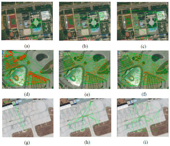
Figure 13.
Delaunay triangulation network of matches from satellite stereo images WX1–3. (a,d,g) tested on ASIFT. (b,e,h) tested on Brown-AffNet. (c,f,i) tested on SJRS-AffNet.

Table 1.
Comparison of the test results of three methods using ground-based, aerial, and satellite images. The best values are highlighted in bold.
- (1)
- The SJRS-AffNet method had advantages, with respect to the number of correct matching points and the match correct rate. There was a significant increase in the number of matching points in JJ1–2 in Figure 8; HK1 and HK3 in Figure 9; and WX1–2 in Figure 10. Figure 8, Figure 9 and Figure 10 show that SJRS-AffNet could obtain more matching point pairs for most test data. Table 1 also reveals that SJRS-AffNet was oriented toward wide-baseline weak-texture stereo images and could obtain more matching point pairs in most cases and achieve a higher match correct rate. Compared with Brown-AffNet, SJRS-AffNet had significant advantages because the SJRS dataset had a greater quantity and breadth than the Brown dataset. In particular, the images in the SJRS dataset came from different platforms (aerial, satellite, and ground-based close-range platforms), whereas the images in the Brown dataset were only ground-based close-range images, mainly of artificial statues and natural landscapes. Therefore, the trained SJRS-AffNet was more generalizable than Brown-AffNet.
- (2)
- Table 1 also shows that SJRS-AffNet had advantages with respect to match correct rate when tested on ground-based close-range image data. The reason is that relatively few types of scene texture, such as walls, bare ground, and green space, occur in ground-based close-range images. Therefore, the model trained on this dataset can achieve a higher match correct rate on ground-based close-range images. In contrast, the aerial and satellite photography platforms have larger fields of view, so more types of texture appear in the images in HK1–3 and WX1–3. To improve the match correct rate of such images in the future, it will be necessary to further increase the types and the quantity of textures covered by the SJRS dataset.
- (3)
- SJRS-AffNet had obvious advantages with respect to matching spatial distribution quality. Table 1 shows that SJRS-AffNet can achieve high matching spatial distribution quality for most aerial, satellite, and ground-based close-range images. In Figure 11, especially for JJ1–2, the distribution area in the Delaunay triangulation network was significantly improved; in Figure 12, only the distribution area of the HK1 Delaunay triangulation network was improved more significantly; in Figure 13, the distribution areas of WX1–3 triangular networks were all significantly improved. This result is consistent with the visual global and local matching results shown in Figure 8, Figure 9, Figure 10, Figure 11, Figure 12 and Figure 13. This shows the effectiveness of the matching spatial distribution quality model that considers both global and local images and verifies the superiority of SJRS.
- (4)
- Figure 8, Figure 9, Figure 10, Figure 11, Figure 12 and Figure 13 and Table 1 reveal that there is no method that can adapt to image data from all types of platforms and to images of all terrain textures. The size of the training dataset directly affected the image matching performance of the deep learning model. Although SJRS-AffNet could achieve better matching results for most of the test data, it was not as good as the ASIFT algorithm for individual test images and evaluation metrics. Figure 10 and Figure 13 show that, given the WX3 stereo pair, none of the three methods tested could obtain a large number of matches. The reason is that there are many obvious ground feature differences in the corresponding regions of WX3. Due to the low similarity between the corresponding areas, many corresponding features were eliminated as false matches.
4. Conclusions
This paper proposed an algorithm for the automatic production of a benchmark dataset for affine-invariant feature matching. The algorithm effectively integrated two types of complementary corresponding features, from ASIFT and the deep learning model LoFTR, and generated quasi-dense matches. Matching points with uniform spatial distribution were then selected using the dual constraints of the neighborhood distance threshold and maximum information entropy. Next, the neighborhoods of matching points were automatically extracted, and the corresponding patches were output in batches. The algorithm was used to automatically construct a large-scale SJRS dataset containing images from ground-based close-range, aerial, and satellite sources. Finally, the SJRS and Brown datasets were applied separately to the affine-invariant model AffNet for training. Comprehensive test results showed that SJRS-AffNet had an advantage with respect to the number of matching points and the correct matching rate; moreover, SJRS-AffNet was able to achieve a high matching spatial distribution quality for most of the aerial, satellite, and ground-based close-range images, and SJRS-AffNet could achieve superior performance when matching stereo images with large viewpoint differences and regions with weak texture.
The main contributions of this paper are as follows: (1) an effective algorithm for the production of a deep learning dataset for affine-invariant feature matching; (2) the most extensive deep learning benchmark dataset to date for affine-invariant feature matching; and (3) a distribution evaluation model that considers both global and local image contents to accurately evaluate the spatial distribution quality for matching points. Due to the multi-scale, multi-view, and multi-spectral characteristics of new remote sensing images, it is necessary in future works to construct a very-large-scale benchmark dataset that covers more spectral features and texture types. Another topic for future works is the integration of the self-attention and cross-attention mechanisms into AffNet to improve the universality of the existing matching model for different imaging mechanisms and texture types. Additionally, the current approach has some limitations, such as too few matching points for significant parallax changes and complex 3D scenes; we hope to overcome this insufficiency in the future.
Author Contributions
Conceptualization, Jianya Gong and Guobiao Yao; methodology, Guobiao Yao and Jianya Gong; software, Guobiao Yao and Jin Zhang; data curation, Jin Zhang and Guobiao Yao; validation, Guobiao Yao, Jin Zhang, and Fengxiang Jin; formal analysis, Guobiao Yao and Jianya Gong; writing—original draft preparation, Guobiao Yao; writing—review and editing, Jianya Gong and Fengxiang Jin; supervision, Jianya Gong and Fengxiang Jin. All authors have read and agreed to the published version of the manuscript.
Funding
This work was supported by the National Natural Science Foundation of China with Project No. 42171435, the Shandong Provincial Natural Science Foundation with Project No. ZR2021MD006, the Postgraduate Education and Teaching Reform Foundation of Shandong Province with Project No. SDYJG19115, and the Undergraduate Education and Teaching Reform Foundation of Shandong Province with Project No. Z2021014. This work was also funded by the high quality graduate course of Shandong Province with Project No. SDYKC2022151.
Institutional Review Board Statement
Not applicable.
Informed Consent Statement
Informed consent was obtained from all subjects involved in the study.
Data Availability Statement
The case data can be downloaded from GitHub https://github.com/Zhangjin0357/SJRS (accessed on 5 July 2022).
Acknowledgments
The authors would like to thank Jean-Michel Morel, Jiaming Sun, and Dmytro Mishkin for providing their key algorithms.
Conflicts of Interest
The authors declare no conflict of interest.
References
- Wierzbicki, D.; Nienaltowski, M. Accuracy analysis of a 3D model of excavation, created from images acquired with an action camera from low altitudes. ISPRS Int. J. Geo-Inf. 2019, 8, 83. [Google Scholar] [CrossRef]
- Yao, G.B.; Yilmaz, A.; Meng, F.; Zhang, L. Review of wide-baseline stereo image matching based on deep learning. Remote Sens. 2021, 13, 3247. [Google Scholar] [CrossRef]
- Lin, C.; Heipke, C. Deep learning feature representation for image matching under large viewpoint and viewing direction change. ISPRS J. Photogramm. Remote Sens. 2022, 190, 94–112. [Google Scholar] [CrossRef]
- Sofie, H.; Bart, K.; Revesz, P.Z. Affine-invariant triangulation of spatio-temporal data with an application to image retrieval. Int. J. Geo-Inf. 2017, 6, 100. [Google Scholar] [CrossRef]
- Ma, J.; Sun, Q.; Zhou, Z.; Wen, B.; Li, S. A Multi-scale residential areas matching method considering spatial neighborhood features. ISPRS Int. J. Geo-Inf. 2022, 11, 331. [Google Scholar] [CrossRef]
- Kızılkaya, S.; Alganci, U.; Sertel, E. VHRShips: An extensive benchmark dataset for scalable deep learning-based ship detection applications. ISPRS Int. J. Geo-Inf. 2022, 11, 445. [Google Scholar] [CrossRef]
- Brown, M.; Hua, G.; Winder, S. Discriminative learning of local image descriptors. IEEE Trans. Pattern. Anal. Mach. Intell. 2011, 33, 43–57. [Google Scholar] [CrossRef]
- David, G.L. Distinctive image features from scale-invariant keypoints. Int. J. Comput. Vision. 2004, 60, 91–110. [Google Scholar] [CrossRef]
- Fischler, M.A.; Bolles, R.C. Random sample consensus: A paradigm for model fitting with applications to image analysis and automated cartography. Commun. ACM 1981, 24, 381–395. [Google Scholar] [CrossRef]
- Yang, H.; Zhang, S.; Wang, L. Robust and precise registration of oblique images based on scale-invariant feature transformation algorithm. IEEE Geosci. Remote Sens. Lett. 2012, 9, 783–787. [Google Scholar] [CrossRef]
- Zhang, Q.; Wang, Y.; Wang, L. Registration of images with affine geometric distortion based on maximally stable extremal regions and phase congruency. Image Vis. Comput. 2015, 36, 23–39. [Google Scholar] [CrossRef]
- Xiao, X.W.; Guo, B.X.; Li, D.R.; Zhao, X.A. Quick and affine invariance matching method for oblique images. Acta Geod. Et Cartogr. Sin. 2015, 44, 414–442. [Google Scholar] [CrossRef]
- Xiao, X.W.; Li, D.R.; Guo, B.X.; Jiang, W.T. A robust and rapid viewpoint-invariant matching method for oblique images. Geomat. Inf. Sci. Wuhan Univ. 2016, 41, 1151–1159. [Google Scholar] [CrossRef]
- Jiang, S.; Xu, Z.H.; Zhang, F.; Liao, R.C.; Jiang, W.S. Solution for efficient SfM reconstruction of oblique UAV images. Geomat. Inf. Sci. Wuhan Univ. 2019, 44, 1153–1161. [Google Scholar] [CrossRef]
- Morel, J.-M.; Yu, G. Asift: A new framework for fully affine invariant image comparison. SIAM J. Imaging Sci. 2009, 2, 438–469. [Google Scholar] [CrossRef]
- Yao, G.B.; Yilmaz, A.; Zhang, L.; Meng, F.; Ai, H.B.; Jin, F.X. Matching large baseline oblique stereo images using an end-to-end convolutional neural network. Remote Sens. 2021, 13, 274. [Google Scholar] [CrossRef]
- Liu, J.; Ji, S.P. Deep learning based dense matching for aerial remote sensing images. Acta Geod. Cartogr. Sin. 2019, 48, 1141–1150. [Google Scholar] [CrossRef]
- Tian, Y.R.; Fan, B.; Wu, F.C. L2-net: Deep learning of discriminative patch descriptor in euclidean space. In Proceedings of the IEEE Conference on Computer Vision and Pattern Recognition, Honolulu, HI, USA, 21–26 July 2017; pp. 661–669. [Google Scholar] [CrossRef]
- Mishchuk, A.; Mishkin, D.; Radenovic, F. Working hard to know your neighbor’s margins: Local descriptor learning loss. Adv. Neural Inf. Process. Syst. 2017, 1, 4826–4837. [Google Scholar] [CrossRef]
- Mishkin, D.; Radenovic, F.; Matas, J. Repeatability is not enough: Learning affine regions via discriminability. In Proceedings of the 2018 Computer Vision, Munich, Germany, 8–14 September 2018; pp. 287–304. [Google Scholar] [CrossRef]
- Sarlin, P.-E.; DeTone, D.; Malisiewicz, T.; Rabinovich, A. SuperGlue: Learning feature matching with graph neural networks. In Proceedings of the IEEE 2020 Conference on Computer Vision and Pattern Recognition (CVPR), Seattle, WA, USA, 14–19 June 2020. [Google Scholar] [CrossRef]
- Vaswani, A.; Shazeer, N.; Parmar, N.; Uszkoreit, J.; Jones, L.; Gomez, A.N.; Kaiser, L.; Polosukhin, I. Attention is all you need. arXiv 2017, arXiv:1706.03762. [Google Scholar] [CrossRef]
- Sun, J.; Shen, Z.; Wang, Y.; Bao, H.; Zhou, X. LoFTR: Detector-free local feature matching with transformers. arXiv 2021, arXiv:2104.00680. [Google Scholar] [CrossRef]
- Balntas, V.; Lenc, K.; Vedaldi, A.; Mikolajczyk, K. HPatches: A benchmark and evaluation of handcrafted and learned local descriptors. In Proceedings of the 2017 IEEE Conference on Computer Vision and Pattern Recognition (CVPR), Honolulu, HI, USA, 21–26 July 2017; pp. 3852–3861. [Google Scholar]
- Li, Z.; Snavely, N. MegaDepth: Learning single-view depth prediction from internet photos. In Proceedings of the Computer Vision and Pattern Recognition (CVPR), Salt Lake City, UT, USA, 18–23 June 2018. [Google Scholar]
- Yao, G.B.; Deng, K.Z.; Zhang, L. An automated registration method with high accuracy for oblique stereo images based on complementary affine invariant features. Acta Geod. Cartogr. Sin. 2013, 42, 869–876. [Google Scholar]
- Li, X.; Yang, Y.H.; Yang, B.; Yin, F.A. Multi-source remote sensing image matching method using directional phase feature. Geomat. Inf. Sci. Wuhan Univ. 2020, 45, 488–494. [Google Scholar] [CrossRef]
- Yuan, X.X.; Yuan, W.; Chen, S.Y. An automatic detection method of mismatching points in remote sensing images based on graph theory. Geomat. Inf. Sci. Wuhan Univ. 2018, 43, 1854–1860. [Google Scholar] [CrossRef]
- Zhu, Q.; Wu, B.; Xu, Z.X. Seed point selection method for triangle constrained image matching propagation. IEEE Geosci. Remote Sens. Lett. 2006, 3, 207–211. [Google Scholar] [CrossRef]


Disclaimer/Publisher’s Note: The statements, opinions and data contained in all publications are solely those of the individual author(s) and contributor(s) and not of MDPI and/or the editor(s). MDPI and/or the editor(s) disclaim responsibility for any injury to people or property resulting from any ideas, methods, instructions or products referred to in the content. |
© 2023 by the authors. Licensee MDPI, Basel, Switzerland. This article is an open access article distributed under the terms and conditions of the Creative Commons Attribution (CC BY) license (https://creativecommons.org/licenses/by/4.0/).