Identification of Urban Functional Zones Based on the Spatial Specificity of Online Car-Hailing Traffic Cycle

Abstract

The study of urban functional zoning is not only important for analyzing urban spatial structure but also for optimizing urban management and promoting scientific urban planning. Different areas undertaking different urban functions correspond to different traffic patterns and specific cycles. Here, a method named Urban Functional Zoning based on the Spatial Specificity (UFZ-SS) is proposed. The core of this method is to obtain urban spatial zoning through the specific cycles of traffic flows. First, UFZ-SS uses the Ensemble Empirical Modal Decomposition (EEMD) method to extract the specific periodic signal characteristics of traffic flows. Second, UFZ-SS calculates the contribution of online car-hailing traffic of different cycles in each zone. Then, the Gaussian Mixture Model (GMM) is utilized to classify all spatial zones into different spatial partitions based on the contribution of each periodic signal. Finally, this study validates UFZ-SS with the online car-hailing traffic volume in northeast Chengdu, China. The results show that the periodic characteristics of traffic can be effectively extracted and analyzed by the EEMD method, and highly distinct and accurate urban spatial partitioning results can be derived by spatial clustering based on the measures of specific cycles. Moreover, with the assistance of Point of Interest (POI) data, we verify the functional zones and structural patterns, which further demonstrates the validity and rationality of urban functional zones identified by UFZ-SS. This study provides a new potential perspective for the identification of urban functional zones, which may lead to a better understanding of the urban spatial structure and even urban planning.

1. Introduction

Cities are complexes composed of multiple spatial subregions with different functions. The spatial areas with different functions form different city spaces [1], which are closely related to various aspects of urban components, such as residents’ living patterns and urban management and planning [2,3]. The study of urban functional zoning is mainly to spatially divide the whole city through crowdsourcing urban data, to obtain multiple spatial subregions with similar urban characteristics (e.g., population, economy, transportation, etc.) or similar urban functions (e.g., housing, entertainment, education, etc.), and then to illustrate urban spatial structures [4]. It can further reshape people’s perception of urban spatial patterns [5], improve the efficiency of urban organization and resource utilization [6], and then promote scientific urban planning as a whole [7].

Traditionally, the function of different urban places is mostly influenced by development planning and policies. With the continuous improvement of the inner-city infrastructure and urban evolution, urban functional regions may have changed. The impact of traffic on the functional zones of the city is gradually increasing. The different accessibility of land in different areas within the city may lead to differences in human activities and thus the development of different functional zones [8]. Thus, it is difficult to describe the spatial pattern of the city in the new stage merely through the administrative zoning of the city, which also makes it difficult to meet the needs of the continuous development of the city [9,10]. It is now highly necessary to study the functional zoning of the city space.

With the development of location/activity sensing technologies and location-based services, multiple data types have emerged and are widely used in urban research [11]. In addition to inheriting the “5Vs” (volume, velocity, value, variety, and veracity) of big data, big data in cities has the attributes of time and space, indicating human movements, spatial interactions, and human–land relationships [12]. The availability of these data and methods offers the possibility to explore the travel patterns and social behaviors of residents, identify the spatial functions within cities, and analyze the spatial structure of cities. Current research on dynamic urban spatial zoning takes temporal information into account and utilizes temporal change patterns for spatial structure identification, but generally ignores the periodic specificity of flow data. The traffic flow can be viewed as a spectrum that is superimposed by multiple periods, and urban regions that undertake different functions may have different periodic patterns for their traffic flows. For example, for working and living areas, there may be a longer period of traffic flow evolution patterns due to daily work and life. For commercial and entertainment areas, the large number of recreational and production activities makes the movement of people and goods more frequent and the corresponding traffic flow period shorter. These idiosyncratic periodic components are often buried by the dominant urban periodic patterns on large time scales. Thus, the extraction and analysis of time-varying periods for flow data from different regions incorporate the dynamics and periodicity of temporal data, with better disclosing of the functional zoning of urban space.

Online car-hailing is an emerging urban sharing economy application, connecting users’ demand and supply, which allows passengers to call and ride vehicles [13]. The data gathered from online car-hailing indicates the actual trajectory information, including location and time, which becomes a new source of information that can be used to study people’s travel behavior and urban mobility [14]. Due to the direct navigation and point-to-point characteristics, online car-hailing trips can reflect the main characteristics of residents’ traffic travel behavior in different areas within the city. Therefore, it is possible to use high-frequency time series and high-spatial resolution data of online car-hailing traffic to accurately reveal the evolution characteristics and patterns of traffic.

This paper attempts to improve the research in the field of urban functional zoning by focusing on the extraction and specificity measurement of time-varying periodic signals of traffic flows in different city spaces, then applying them to the delineation and identification of urban functional zones. The scenario being studied is shown in Figure 1. In this paper, a method named Urban Functional Zoning based on the Spatial Specificity (UFZ-SS) is proposed. Firstly, the original time series of online car-hailing flows is decomposed by the signal processing method, and the multi-periodic signals in the series are extracted. Then, a new method is proposed to measure the contribution of the extracted periodic signals, and a contribution matrix is constructed based on the specificity measures of multiple periodic signals in different units. A clustering algorithm is used to obtain the spatial zoning based on periodic signal characterizations of every location. Finally, the functions undertaken by different zones are explored in conjunction with POI data to interpret the functional zones and structural patterns within the city. The contributions of this paper are: (i) This paper innovatively uses the temporal dynamics and periodicity patterns of online car-hailing traffic for the identification of urban functional zones. (ii) This paper proposes the method of measuring the contribution of different periodic signals in the original traffic sequences. (iii) This paper reveals the specificity of the temporal change period of online car-hailing traffic in different regions, and then provides a new idea and method for insight into urban functional zoning and urban dynamic structure, which is useful for urban planning and traffic management.

The structure of the paper is as follows. In Section 2, a comprehensive review of related works is performed to introduce the usage of online car-hailing data and the methods of urban functional zoning. In Section 3, the research methods used in this paper are presented. A case study is contained in Section 4, and Section 5 provides the discussions and conclusions about this study.

2. Related Works

2.1. Online Car-Hailing Data

The car-hailing data for the traditional study was obtained by checkpoints, which was greatly limited by the survey actions. With the availability of Global Positioning System (GPS) trajectory data, researchers have a better way to study online car-hailing and the application of the data. For example, Brockman and Theis [15] used trackable items (known as travel bugs) to discover human mobility patterns. Doyle et al. [16] used cell phone data to analyze the urban residents’ behaviors. Pieroni et al. [17] used smart card data to explore the population travel patterns.

Trajectory data from online car-hailing services have been popular due to the emergence of a large number of online taxi-hailing activities. Such data are characterized by high accuracy, good continuity, and a high degree of automation, and can reveal the behavioral patterns and spatio-temporal patterns of urban residents [18]. Due to the above advantages, researches have been conducted with the usage of online car-hailing GPS data. Hu et al. [19] classified the city functional zones with the online car-hailing data and deep learning technology. Bogaerts et al. [20] used taxi GPS data to forecast short-term and long-term traffic. Dokuz [21] developed an algorithm using New York taxi GPS data to estimate traffic speed. Loo and Huang [22] introduced a method to identify traffic congestion areas with taxi GPS data and tested it in Asian cities. Huang et al. [23] studied the relationship between people’s ride splitting willingness to spatiotemporal conditions. However, researches on online car-hailing hardly concentrate on the characteristics of periodic feature. The periodic feature may help to reveal potential city information, so we chose to use online car-hailing GPS data in our research.

2.2. Identifying Urban Functional Zones

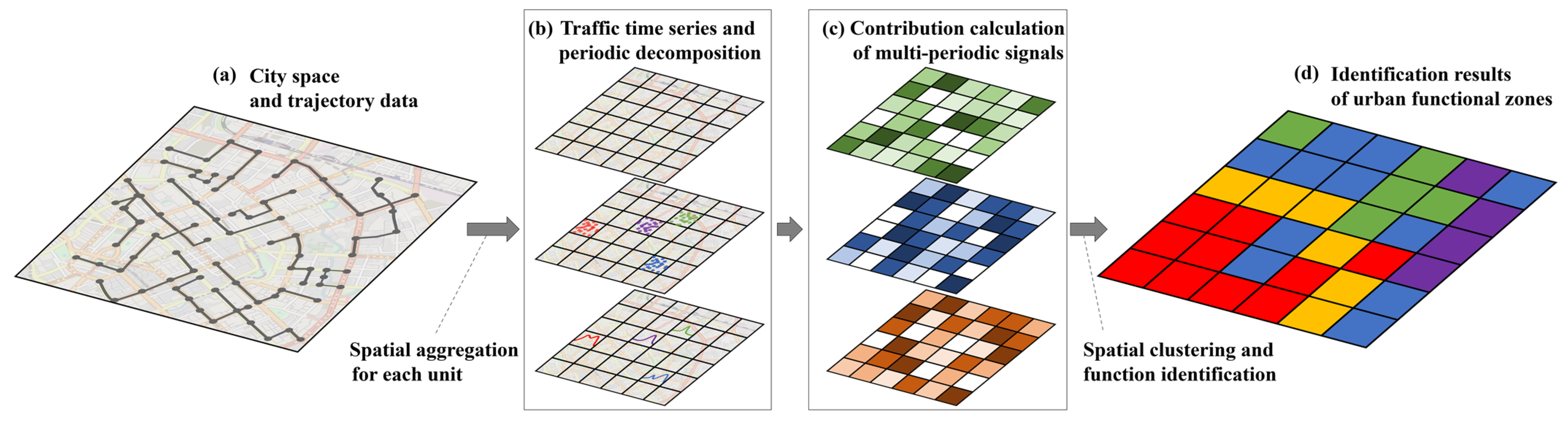
The rapid development of urban modernization has led to the increasing popularity of sensing technologies [24], intelligent transportation systems [25], and location-based services [26], which provide a large amount of geographic data for urban functional zoning. Corresponding zoning and visualization systems have also been developed to promote the development of urban functional zoning [27,28]. By identifying and zoning urban spatial patterns, people can discover the physical characteristics and social attributes of cities, and can enable valuable applications such as urban planning [29].

Herold et al. [30] constructed landscape metrics from spatial information of remote sensing images, then analyzed the urban land structures and changes under urban growth in the urban region of Santa Barbara, California. Gao et al. [31] used social media check-in data to construct a popularity-based probabilistic topic model to extract semantic feature themes for 10 urban areas in the US. Crivellari and Resch [32] used taxi Origin-Destination (OD) flows in New York City combined with local POI-distribution data, and then applied multi-dimensional vector representations of urban areas to identify homogenous functional areas of the city. Bike sharing OD data are also applied in discovering spatiotemporal patterns for revealing urban dynamics [33,34]. Nevertheless, such studies are conducted from a static perspective. Most of them use static information such as remote sensing images or land use data, either assume that the data is equal in temporal characteristics such as POI data, or only consider information on state changes at a single point in time such as OD flows. The resulting static semantics often yield isolated insights [35], failing to express the dynamic characteristics of urban spatial zoning.

Then, some researchers have considered a temporal perspective. They consider the continuity and integrity of crowd movements in their study and also focus on the temporal consistency of the multi-source data. Cai et al. [36] partitioned Tencent location big data by hour, day, and space, then applied tensor factorization to extract conditional probabilities under different modes, thus inferred spatial structure information. Ratti et al. [37] described the use of cell phone data at 5 min or 10 min intervals for a case study in the metropolitan area of Milan, Italy. Peungnumsai et al. [38] combined questionnaire survey data and taxi probe data with a 3–5 s sampling frequency for the service area zoning of cabs in the Bangkok metropolitan area, which also revealed the functional zoning structure of the city to some extent.

It can be seen that urban dynamic spatial zoning considers temporal information and uses the law of temporal changes for spatial structure identification, but generally ignores the spatial specificity of the traffic cycle. The time-varying traffic volume is a complex time series composed of multi-periodic signals. Using the periodic signal analysis method of time series, multiple potential periods of traffic volume time series at different locations can be obtained. Measuring the contribution of different periodic signals to the original time series can indicate the specificity of the periodic signals, thus improving the research in the field of urban functional zoning from the perspective of dynamism and periodicity.

3. Methodology

This study uses the EEMD method to decompose the traffic flow and obtain periodic signals. Then, we construct the contribution matrix by the average proportion method devised in this research to obtain the contribution of different periods of traffic volume on different spatial units. Based on the characteristics of the contribution of each zone in the study area, a machine learning clustering method of GMM is selected to achieve the high-precision clustering of urban functional zones.

Table 1. Descriptions of mathematical symbols.

Symbol	Description
$\mathrm{x}\left(\mathrm{t}\right)$	original time series at t
${\mathrm{n}}_{\mathrm{i}}\left(\mathrm{t}\right)$	the ith superimposed white noise sequence at t
${\mathrm{x}}_{\mathrm{i}}\left(\mathrm{t}\right)$	additional noise signal of the ith trial at t
${\mathrm{c}}_{\mathrm{i},\mathrm{j}}\left(\mathrm{t}\right)$	the jth IMF component obtained from the decomposition after the ith addition of white noise at t
${\mathrm{r}}_{\mathrm{i},\mathrm{J}}\left(\mathrm{t}\right)$	residual function after the ith addition of white noise at t
${\mathrm{IMF}}_{\mathrm{j}}\left(\mathrm{t}\right)$	value of the jth IMF of the EEMD decomposition
${\mathrm{Con}}_{\mathrm{k},\mathrm{j}}$	contribution of the jth IMF component in the kth space unit
${\mathrm{IMF}}_{\mathrm{k},\mathrm{j}}\left(\mathrm{t}\right)$	value of the jth IMF component in the kth space unit at t
${\mathrm{TS}}_{\mathrm{k}}\left(\mathrm{t}\right)$	value of the original time series with grid number k at t
${\mathrm{L}}_{\mathrm{k}}$	length of the time series at grid number k
${\mathsf{\phi }}_{\mathrm{i}}$	weight parameter of the ith Gaussian distribution in the mixture model
${\mathsf{\mu }}_{\mathrm{i}}$	mean matrices of the ith Gaussian distribution in the mixture model
${\mathsf{\Sigma }}_{\mathrm{i}}$	covariance matrices of the ith Gaussian distribution in the mixture model

provides the descriptions of the mathematical symbols used in this paper.

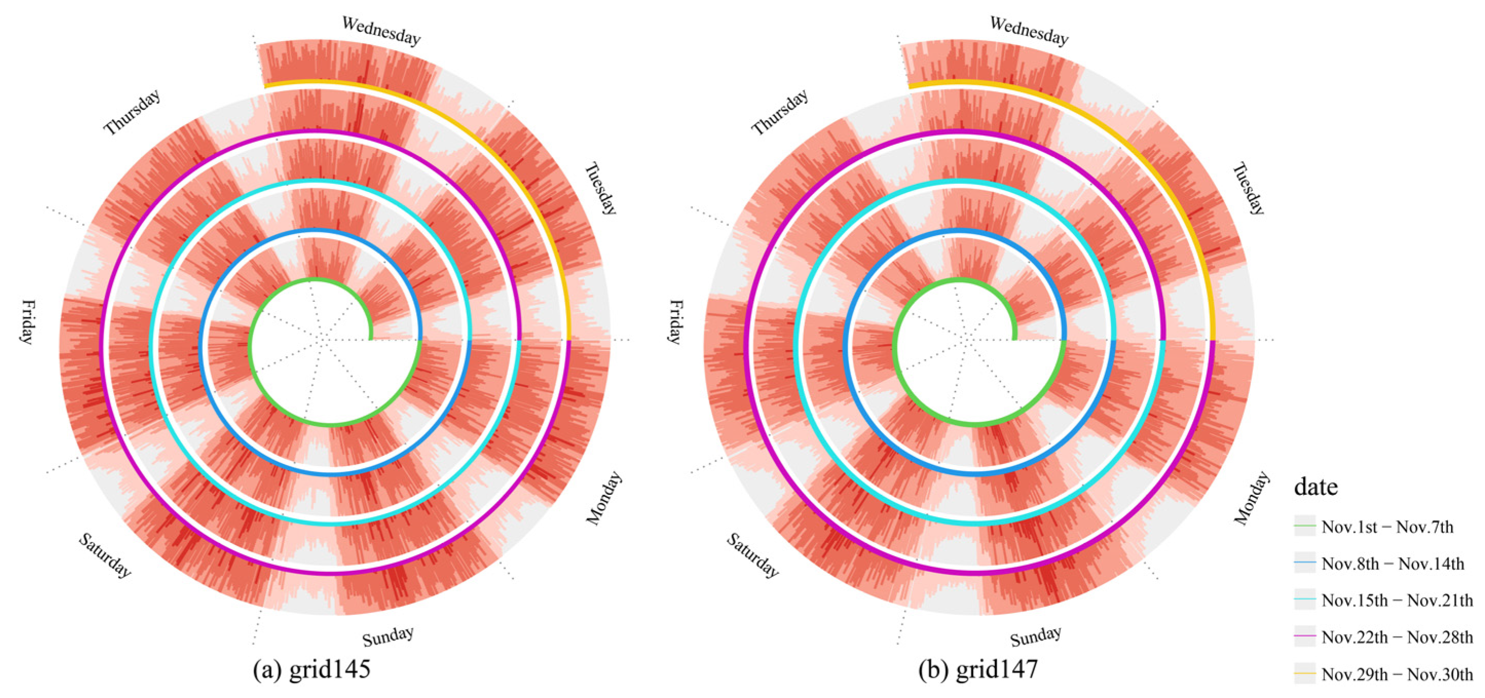
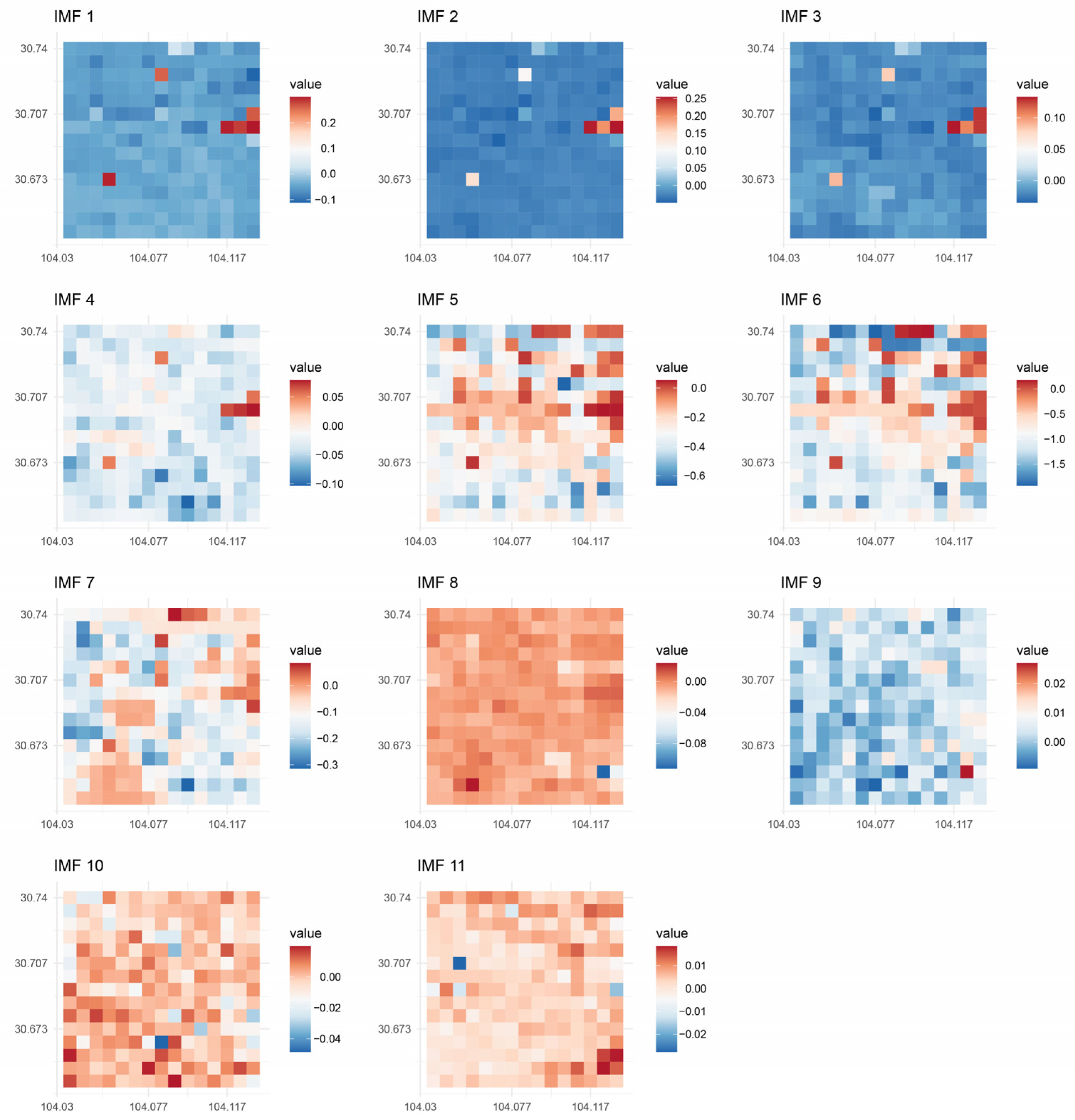
3.1. Online Car-Hailing Traffic Period Analysis

The traffic volume time series are complex signals composed of different periodic signal sequences. The periodic signal sequences, in addition to common cycles such as daily and weekly, have implied periods that can reflect the potential social fingerprint information. EEMD is an improved method of EMD (Empirical Mode Decomposition), which can effectively solve the modal confounding phenomenon in the EMD method by introducing uniformly distributed white noise several times in the modal decomposition process and performing ensemble averaging [39]. By decomposing the time series through EEMD, different Intrinsic Mode Function (IMF) components with specific periods can be obtained.

The algorithm of EEMD is as follows and Figure 2 is its flow chart:

(1) Set the number of times the time series is processed: M,

(2) Stack a series of white noise ${\mathrm{n}}_{\mathrm{i}}\left(\mathrm{t}\right)$ with normal distribution onto the original time series x(t) to produce a new time series:

$${\mathrm{x}}_{\mathrm{i}}\left(\mathrm{t}\right)=\mathrm{x}\left(\mathrm{t}\right)+{\mathrm{n}}_{\mathrm{i}}\left(\mathrm{t}\right),$$

(1)

where ${\mathrm{n}}_{\mathrm{i}}\left(\mathrm{t}\right)$ denotes the ith superimposed white noise sequence, ${\mathrm{x}}_{\mathrm{i}}\left(\mathrm{t}\right)$ denotes the additional noise signal of the ith trial, $\mathrm{i}=1,2,\dots ,\mathrm{M}.$

(3) Decompose the noisy signal into EMD components and obtain a series of IMF components:

$${\mathrm{x}}_{\mathrm{i}}(\mathrm{t})={{\displaystyle \sum }}_{\mathrm{j}=\mathrm{1}}^{\mathrm{J}}{\mathrm{c}}_{\mathrm{i},\mathrm{j}}(\mathrm{t})+{\mathrm{r}}_{\mathrm{i},\mathrm{J}}(\mathrm{t}),$$

(2)

where ${\mathrm{c}}_{\mathrm{i},\mathrm{j}}\left(\mathrm{t}\right)$ is the jth IMF component obtained from the decomposition after the ith addition of white noise, ${\mathrm{r}}_{\mathrm{i},\mathrm{J}}\left(\mathrm{t}\right)$ is the residual function representing the average trend of the signal, and J is the number of IMF components.

(4) Repeat steps (2) and (3) for M times and add white noise signals with different amplitudes during each decomposition to obtain the set of IMF components:

$${\mathrm{c}}_{1,\mathrm{j}}\left(\mathrm{t}\right),{\mathrm{c}}_{2,\mathrm{j}}\left(\mathrm{t}\right),\dots ,{\mathrm{c}}_{\mathrm{M},\mathrm{j}}\left(\mathrm{t}\right),\mathrm{j}=1,2,\dots ,\mathrm{J},$$

(3)

$${\mathrm{IMF}}_{\mathrm{j}}(\mathrm{t})=\frac{1}{\mathrm{M}} {{\displaystyle \sum }}_{\mathrm{i}=\mathrm{1}}^{\mathrm{M}}{\mathrm{c}}_{\mathrm{i},\mathrm{j}}(\mathrm{t}),$$

(4)

where ${\mathrm{IMF}}_{\mathrm{j}}\left(\mathrm{t}\right)$ is the jth IMF of the EEMD decomposition, $\mathrm{i}=1,2,\dots ,\mathrm{M},\mathrm{j}=1,2,\dots ,\mathrm{J}.$

3.2. Signal Specificity Measurements of Different Periods

Among the IMF components decomposed by the EEMD algorithm, some low-frequency components are usually pseudo components, which need to be further distinguished. The traditional methods may not consider the above low-frequency components enough and ignore their intrinsic meanings. Especially in traffic volume, each IMF component represents a potential periodic feature of the study area and should not be treated in a simple and non-differentiated way. Therefore, a contribution index is proposed in this study to calculate the contribution of IMF components deposed from the time series of the grid.

In the signal processing field, algorithms for determining and screening IMF component signals include the correlation coefficient method [40], KL scatter method [41], energy-based method [42], and power spectral density-based method [43], etc. Some scholars have also combined multiple indicators to obtain a sensitivity index [44], which is used to determine the IMF components and their contribution to the original sequence. To exploit the potential advantage of the IMF components derived from the EEMD decomposition over the original series cycle, we propose a ratio-defined contribution assignment method based on traffic flow characteristics: the average proportion method. In this study, the contribution measure algorithm is constructed by performing a ratio operation between different IMF component values and the contemporaneous values of the original time series. Then this study uses the average ratio as the contribution of the IMF component to the original time series. Based on this method, the contribution measure can be calculated by the following equation:

$${\mathrm{Con}}_{\mathrm{k},\mathrm{j}}={{\displaystyle \sum }}_{\mathrm{t}=\mathrm{1}}^{\mathrm{n}}\frac{{\mathrm{IMF}}_{\mathrm{k},\mathrm{j}}\left(\mathrm{t}\right)}{{\mathrm{TS}}_{\mathrm{k}}\left(\mathrm{t}\right)}/{\mathrm{L}}_{\mathrm{k}},$$

(5)

where ${\mathrm{Con}}_{\mathrm{k},\mathrm{j}}$ represents the contribution of the jth IMF component in the kth space unit. ${\mathrm{IMF}}_{\mathrm{k},\mathrm{j}}\left(\mathrm{t}\right)$ represents the value of the jth IMF component in the kth space unit at moment t. ${\mathrm{TS}}_{\mathrm{k}}\left(\mathrm{t}\right)$ represents the value of the original time series with grid number k at moment t. ${\mathrm{L}}_{\mathrm{k}}$ represents the length of the time series at grid number k.

3.3. Urban Spatial Partition and Function Identification

By adopting the above contribution calculation method, this paper constructs the contribution matrix to show the contribution relationship between each IMF component and the original time series, uses the GMM to classify all spatial locations into different types, and verifies the urban functions undertaken by different spatial areas based on the POI data.

3.3.1. Periodic Contribution Matrix

By adopting the above contribution calculation method, this study constructs the contribution matrix ${\mathrm{Con}}_{\mathrm{IMF}}$ to show the contribution relationship between each IMF component and the original time series:

$${\mathrm{Con}}_{\mathrm{IMF}}=[\begin{array}{cccc}{\mathrm{Con}}_{11}& {\mathrm{Con}}_{12}& \cdots & {\mathrm{Con}}_{1\mathrm{n}}\\ {\mathrm{Con}}_{21}& {\mathrm{Con}}_{22}& \cdots & {\mathrm{Con}}_{2\mathrm{n}}\\ ⋮& ⋮& \ddots & ⋮\\ {\mathrm{Con}}_{\mathrm{m}1}& {\mathrm{Con}}_{\mathrm{m}2}& \cdots & {\mathrm{Con}}_{\mathrm{m}\mathrm{n}}\end{array}],$$

(6)

where ${\mathrm{Con}}_{\mathrm{k},\mathrm{j}}$ is the contribution of the jth IMF component with grid number k, the number of grids is m, and the number of IMF components is n, $\mathrm{k}=1,2,\dots ,\mathrm{m},\mathrm{j}=1,2,\dots ,\mathrm{n}.$

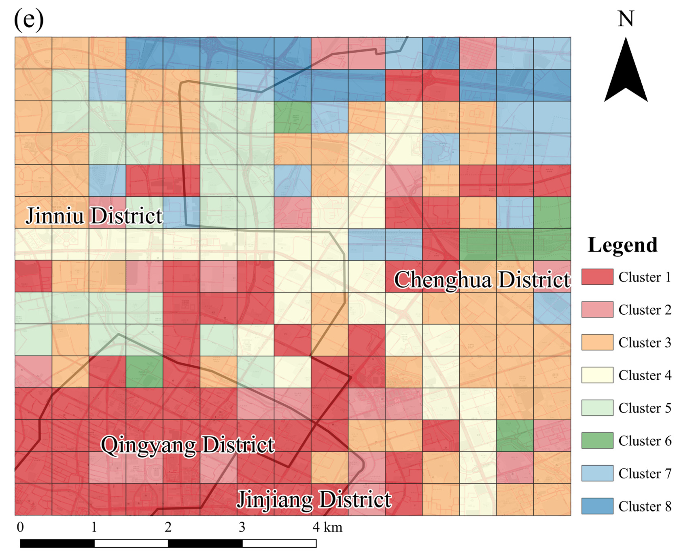
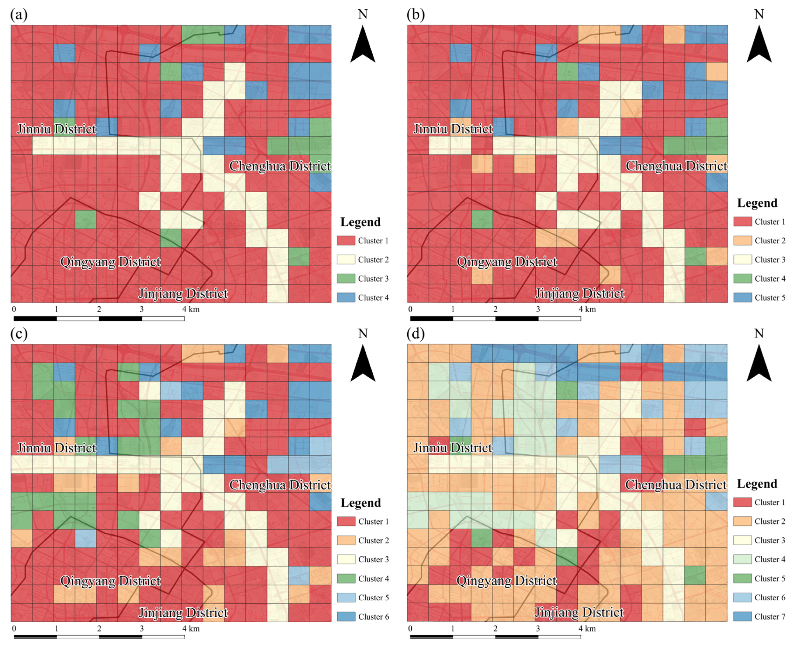
3.3.2. Spatial Clustering

Based on the obtained contribution matrix, this study uses time series clustering to obtain the land partition pattern of the study area. Time series clustering can be broadly divided into methods based on original measures and features [45]. Feature-based time series clustering takes data dimensionality reduction as the guiding idea and takes features of the data’s internal characteristics as the input, effectively solving the clustering problems of high-dimension data, missing data, unequal data length, and low sensitivity to noisy data. Besides, it overcomes the problem of noise unevenness in the decomposition of IMF components by the EEMD algorithm [46]. We cluster the periodic component contribution to the original sequence based on GMM and evaluate the performance of each model by calculating the Bayesian Information Criterion (BIC) value of each clustering result to determine the best model type and the best number of clusters. Then the clustering results are used to divide the spatial partition of the study area, which provides a more comprehensive and effective analysis of traffic flows and urban operation patterns.

The principle of the GMM is as follows: GMM uses combinations of Gaussian distributions to describe the data distribution. Each Gaussian model represents a cluster and assigns the data to different models based on probability. Let the contribution be X, which is composed of K Gaussian distributions. GMM is expressed as follows:

$$\mathrm{P}(\mathrm{x}|\mathsf{\theta })={{\displaystyle \sum }}_{\mathrm{i}=1}^{\mathrm{K}}{\mathsf{\phi }}_{\mathrm{i}}\frac{1}{\sqrt{2\mathsf{\pi }{\mathsf{\Sigma }}_{\mathrm{i}}}}{\mathrm{e}}^{-\frac{{(\mathrm{x}-{\mathsf{\mu }}_{\mathrm{i}})}^2}{2{\mathsf{\Sigma }}_{\mathrm{i}}}},$$

(7)

where ${\mathsf{\phi }}_{\mathrm{i}}$ represents the weight parameter of the ith Gaussian distribution in the mixture model species, with a total of K, and their sum is 1. ${\mathsf{\mu }}_{\mathrm{i}}$ and ${\mathsf{\Sigma }}_{\mathrm{i}}$ are respectively the mean and covariance matrices under the Gaussian distribution.

The BIC value is defined as:

$$2\log \mathrm{p}(\mathrm{x}|\mathrm{M})+\mathrm{constant}\approx 2{\mathrm{l}}_{\mathrm{M}}(\mathrm{x},\widehat{\mathsf{\theta }})-{\mathrm{m}}_{\mathrm{M}}\log (\mathrm{n})\equiv BIC$$

(8)

3.3.3. Function Identification of Different Zones

For the spatial division method of urban functions based on the spatial specificity of the urban traffic cycle, this study further combines POI data. We count the number of various types of POIs on each grid and average and standardize them from 0 to 1 in turn. Then we summarize the POIs within the same sub-area and identify the main urban functions undertaken by the area by calculating the percentage of each type of POI in it. Finally, we obtain the urban functional divisions of the study area.

4. Case Study

4.1. Data Description and Experimental Configuration

After proposing the UFZ-SS method, Chengdu is selected as a case study for application and analysis in this paper. This subsection focuses on the basic information of the study area, the data source and its processing, and the configuration of the experiment.

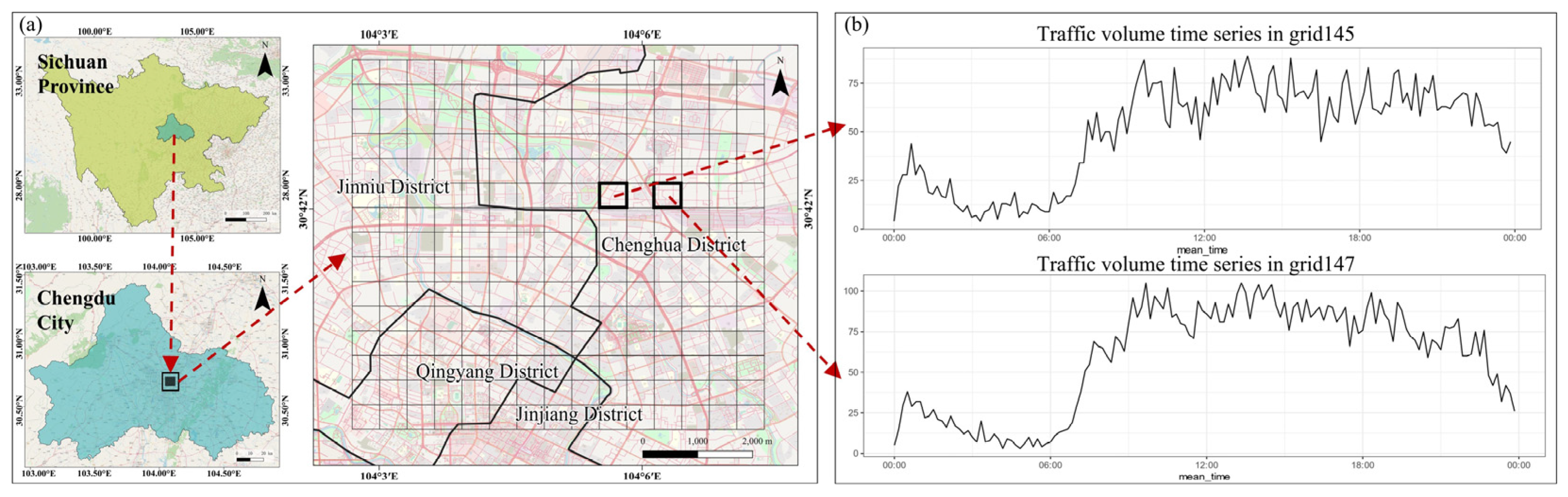
4.1.1. Study Area and Original Data

Chengdu, the capital of Sichuan Province, is a core city in the western area of China, serving as a national high-tech industry base, commerce and logistics center, and comprehensive transportation hub. Chengdu has a circular radial road network. In this paper, a quadrilateral area formed by four points (longitude: 104.04°–104.13°, latitude: 30.65°–30.72°) in the northeast of the fourth ring of Chengdu, whose coordinate system is GCJ-02, is selected for the study. The area consists of the urban land of four municipal districts, namely Qingyang District, Jinniu District, Chenghua District, and Jinjiang District, and is the heart of Chengdu.

The main data used in this paper are the trajectory data of the Didi Chuxing platform in the local area of Chengdu in 2016, from the GAIA open data program KDD CUP 2020 dataset. As the study area is the central area of Chengdu, which is well developed in 2016, and has not changed much, this means that our research based on that data is still indicative. Hence, the trajectory data of November 2016 are selected in this study, and the data volume is about 100 GB. An example of the trajectory data is shown in

Table 2. An example of the trajectory data.

Name	Type	Example	Remark
Driver ID	String	glox.jrrlltBMvCh8nxqktdr2dtopmlH	Desensitized
Order ID	String	jkkt8kxniovIFuns9qrrlvst@iqnpkwz	Desensitized
Timestamp	Int	1501584540	Unix Timestamp(s)
Longitude	Float	104.04392	GCJ-02 Coordinate System
Latitude	Float	30.66703	GCJ-02 Coordinate System

.

4.1.2. Data Processing

In the original data, the driver ID and order ID are encrypted, and the time is stored in Unix timestamp format, which cannot directly meet the requirements of use. Hence, it is necessary to pre-process the data according to their actual situations. The following data pre-processing work is performed in this study: (1) recoding of driver ID and order ID; (2) time conversion from Unix timestamp to Universal Time Coordinated (UTC) time in the format YYYY-MM-DDTHH:mm:ssZ, where Y represents the year, M represents the month, D represents the date, H represents the hour, m represents the minute, s represents the second, T represents the time start, Z represents the time zone. In addition, outlier data are screened from the trajectory data, and trajectories with time intervals longer than 3600 s are excluded to ensure data quality.

The geographic grid is based on a unified, simple spatial division method and spatial coordinate system to partition the region for statistics and analysis of geographic phenomena, which is widely used in the direction of multi-source geospatial data fusion and comprehensive geographic analysis [47]. In this paper, the study area is further divided into 225 grids of 15 × 15 with a spatial resolution of 500 m, which are numbered 1, 2, 3, …, 225 based on the order from left to right and bottom to top. The grid is used as the basic spatial unit for signal decomposition and spatial clustering analysis. The periodic characteristics of the traffic flow on each grid are measured on it. Based on the similarity of the periodic characteristics, different grids can be combined to obtain a comprehensive partition. The study area of this paper is shown in Figure 3a.

After dividing grids, this study superimposes the online car-hailing trajectories with the spatial grids and counts the number of online car-hailing in different periods inside each grid, and the online car-hailing traffic time series in different spatial locations (grids) is aggregated finally. Figure 3b shows the 24 h series of online car-hailing traffic for two representative grids in the study area, numbered 145 and 147, respectively. It shows that the temporal changes of traffic in the two spatially similar areas are similar within a day, where the peak and trough times of the two time series occur close to each other within a day. The duration and transition process of the high and low values are also generally the same, reflecting the diurnal mode of variation. However, the two time series show some differences in terms of the periodicity implied by the peak traffic variation. The overall smaller values and longer intervals between adjacent peaks for grid145 indicate a potentially dominant period in the evolution of traffic flows, while the overall higher values and shorter intervals between adjacent peaks for grid147 indicate a potentially less dominant period in the evolution of traffic flows.

To further demonstrate the periods implied by the temporal variation of data, this study extends the time scale to one month and visualizes the time series by drawing spiral graphs using the spiralize package [48] in R, and the results are shown in Figure 4. From the graph, it can be seen that the temporal variation of the online traffic has obvious periodic characteristics, obeying the repetition of the daily periods, and one or more peak points within each day. Among them, grid145 (Figure 4a) has higher traffic values relative to grid147 (Figure 4b), and the lower value areas are more volatile and more dynamically informative than grid147.

4.1.3. Experimental Configuration

In Section 4.2, this study uses the EEMD method to decompose the time series of the online car-hailing traffic flow into IMF components, and extracts the specific periodic characteristics from IMFs. After that, the method of measuring the specific period of traffic flow over time, the average proportion method, is used to sequentially calculate the contribution of different IMFs to the original time series of traffic flows. Then, the contribution matrix is generated and the spatial visualization is performed. The GMM algorithm is used to classify all spatial grids into different types based on the contribution matrix, and similar types of spatial units can be aggregated into spatial partitions. Finally, this study combines POI data for analysis. By calculating and analyzing the percentage of each POI in different zones, the urban functions undertaken by different spatial partitions are inferred.

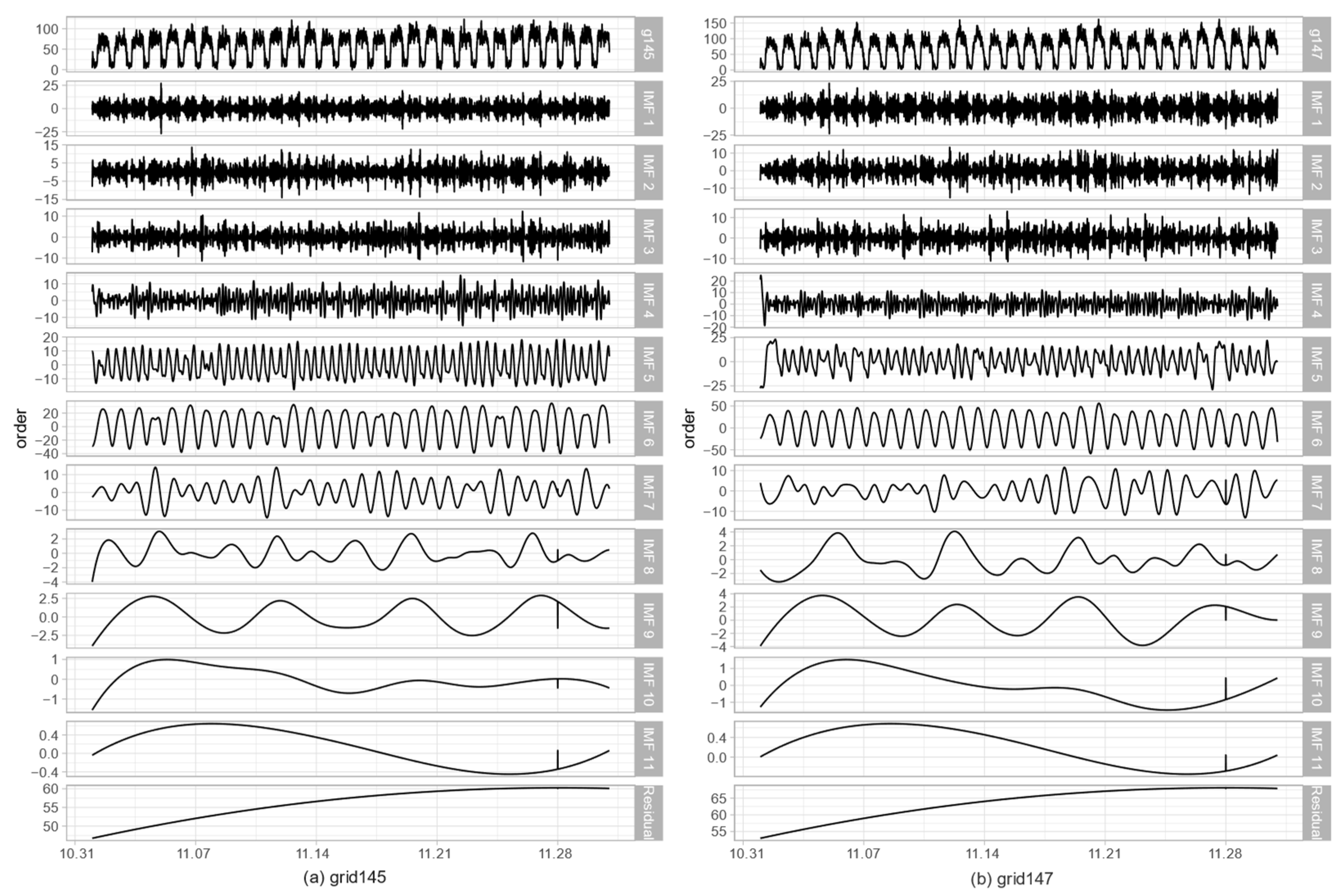
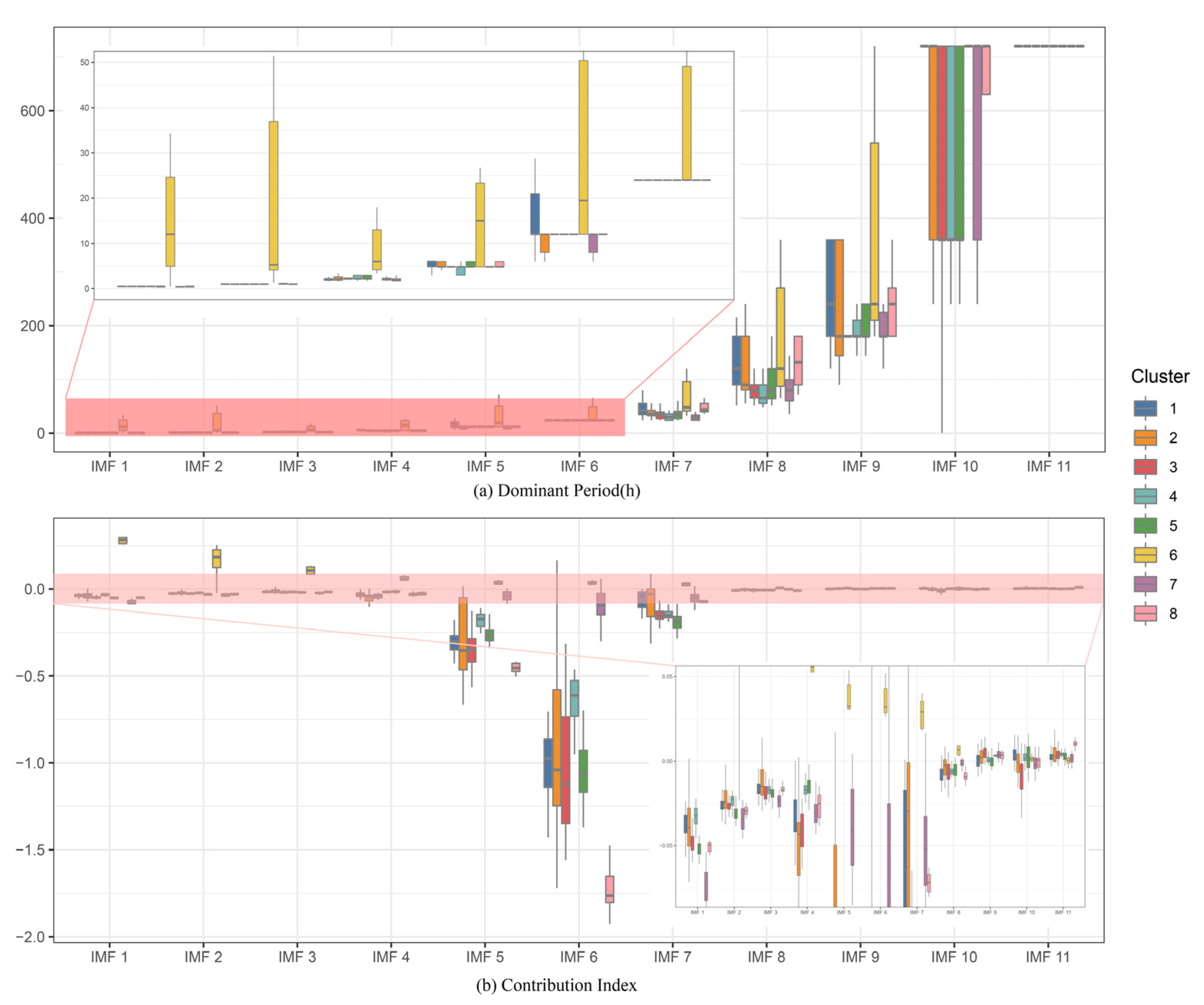
4.2. Periodic Signal Analysis

In this study, the EEMD decomposition is performed separately for each grid cell to extract the IMF components of online car-hailing traffic volume. The results of the EEMD decomposition are demonstrated for grid145 and grid147 as an example. From the decomposition results, it is obvious that EEMD overcomes the endpoint effect and modal confounding problem of EMD well, and is also less computationally intensive than the improved algorithms proposed by researchers afterward, satisfying the requirements of this experiment.

As can be seen from Figure 5, there are fluctuations in the flow series on a day-by-day basis, and the periodic characteristics of the IMF components are evident. Due to the influence of different scales of vertical coordinates, the visualization error at the position of Nov.20th appears, although the difference in instantaneous frequencies corresponding to each IMF component can be visually observed. We quantify the EEMD decomposition results by calculating the principal period and variance contribution of each IMF component, as shown in

Table 3. IMF information for grid145 and grid147.

	grid145		grid147
	Dominant Period (h)	Variance Ratio (%)	Dominant Period (h)	Variance Ratio (%)
IMF 1	0.4999	3.7048	0.4999	2.4684
IMF 2	0.9998	1.2601	0.9998	0.8610
IMF 3	2.9993	1.0458	2.1813	0.7433
IMF 4	4.7989	2.3878	4.7989	1.9501
IMF 5	11.9972	8.0102	11.9972	6.4739
IMF 6	23.9944	46.1930	23.9944	58.5544
IMF 7	23.9944	4.1123	23.9944	1.6154
IMF 8	89.9792	0.1712	179.9583	0.1962
IMF 9	179.9583	0.3137	179.9583	0.2901
IMF 10	719.8333	0.0283	719.8333	0.0519
IMF 11	719.8333	0.0164	719.8333	0.0087

. IMF1–IMF7 all have a principal period within 1 day; IMF1–IMF4, as high-frequency components, have a shorter principal period, reflecting the short-term traffic flow dynamics; IMF5–IMF7 reflect information on the 12 h and 24 h periodic fluctuations of traffic flows; IMF9–IMF11, on the other hand, highlight the general trend of traffic flows in November 2016, with fluctuations remaining stable over time. By calculating the variance ratios of the IMF components, the variance of the 5 h and 0.5 h periodic counterparts are relatively large, except that of IMF5–IMF7. Although the flow morphology is similar between grid145 and grid147, differences in IMF3 and IMF8 are obvious, reflecting the advantages of using EEMD to extract the spatial specificity of the urban traffic cycle.

4.3. Contribution Calculation

Using the average proportion method proposed in this study in Section 3.2, the contribution index of each IMF on each grid is calculated separately.

The results of this study are spatially visualized for the values of IMF’s contribution index, which is shown in Figure 6. It can be seen that the isolated feature areas in the study area are extracted from IMF1–IMF4 components, which are the areas where grid64, grid188, grid133–135, and grid150 are located. In IMF5–IMF7, the agglomerative functional areas of the city are mainly highlighted, such as the 2nd Ring Road of Chengdu in IMF5 and IMF6, and the central area of Chengdu in the lower-left corner of IMF7. For IMF8–IMF11, the contribution values and variance contribution rates are relatively small, spatially scattered, and poorly regular.

4.4. Spatial Partitioning Based on Contribution Matrix of Traffic Flow

In this study, the contribution matrix is clustered using GMM and the number of clusters is determined using BIC values. The relationship between the number of optimal clusters and the variation of BIC values is shown in Figure 7. According to the expectation-maximization algorithm, the larger the BIC value, the better the clustering performance. Therefore, the optimal number of clusters is 8. The BIC value fluctuates up with the growth of the number of clusters until reaching the optimal number of clusters of 8 classes, and fluctuates down thereafter. Under the premise of considering the number of clusters, this study selects the number of clusters from 4 to 8 classes for spatial visualization and display, respectively.

In this study, the above clustering results are spatially visualized and shown in Figure 8. In all five cases, the clustering results can accurately extract parts of the second ring and second ring elevated road areas in Chengdu as a unique cluster, especially in the six and eight cluster results with the highest BIC values. With the second ring and the elevated road area as the division, the rest of the study area is divided to form different clusters. Moreover, as the number of clusters grows, the classification becomes more refined with more special locations extracted, and the areas within the second ring and between the second and third rings are gradually distinguished. However, the specific urban functions of each cluster are not yet known.

In this paper, the classification result with the highest BIC value is analyzed in detail, in which the study area is divided into eight clusters (Cluster 1–Cluster 8). A circular structure is evident in the study area, spreading from the downtown area (lower-left corner of the figure) to the peripheral areas (upper right corner of the figure). Cluster 1 is the most dominant classification result, occupying 58 out of 225 grids. It is mainly in the city center area within the second ring road of Chengdu, showing an obvious spatial correlation between urban traffic flows in a certain area and the dependence of traffic flow on the traffic network. Additionally, there is almost no discrete distribution of clustering results in this cluster. Moreover, Cluster 1 also contains areas such as Qinglongchang Interchange, Chengbei Expressway, and Chuan-Shaan Interchange. This may be because the traffic flow in these areas and the cyclical characteristics of their traffic flow are similar to those of the downtown area. Cluster 2, on the other hand, shows a more discrete character, with its distribution in Chengdu Sports Center, Poly Center, and University of Electronic Science and Technology (Shahe Campus), and there is no regional aggregation. Cluster 3 is mainly distributed in the extensive area in the middle of the second and third ring roads, and the edge of the second ring road, with a small amount distributed on the edge of the first ring road. Cluster 4 can clearly extract the second ring road, the elevated road of the second ring road, and the section of Jiefang Road—Yimajiao Street—Zhaogeosi South Road, which is one of the most important commuting sections in Chengdu, and also reflects the spatial correlation and road network dependence of traffic flows. Cluster 5 is mainly distributed in the northwestern part of the study area, containing part of the northern section of the First Ring Road, Beixing Avenue, Rongbei Trade Avenue, and its surrounding areas. All of these places are closely related to the backbone roads in Chengdu and contain certain regional aggregation characteristics. Cluster 6 occupies the smallest proportion, which is mainly isolated feature areas in the study area, respectively, Grid 64 (Western War Zone Military Area), Grid 188 (Chengdu University Annex area), Grid 44 (Shahe area), Grid 133–135, and Grid 150 (Erxianqiao train storage yard). Cluster 7 is distributed in the northern area outside the Second Ring Road, and the distribution is relatively discrete. Cluster 8 is mainly along the North Third Ring Road of Chengdu, which is divided by the Chuan-Shaan interchange of Cluster 1. In this zone, each subpart is continuous and has a strong road network correlation.

For the spatial clustering results, this subsection further evaluates and analyzes them using the contribution index of each cluster and its dominant period. Firstly, the dominant period and contribution index of each IMF component of each cluster in the spatial partitioning results are calculated independently, as shown in Figure 9. Figure 9a illustrates the dominant period of each IMF component. The horizontal axis of this box plot represents the different IMF components, and the vertical coordinate represents the dominant period in hours. Except for Cluster 6, the periods of each IMF component in each cluster are not exactly the same, but the overall volatility is not significant. For Cluster 6, the degree of volatility is significantly greater from IMF 1 to IMF 9 than for the other groups. Compared to itself, the degree of volatility increases significantly at IMF 8 and IMF 9. It might be due to the fact that Cluster 6 has the smallest proportion of the study area with a little amount of trajectory data. Then the dominant periods of different IMF components are discussed. For IMF 1, its main period is about 0.5 h, IMF 2’s period is about 1 h, and IMF 3’s is about 2.3 h, showing the characteristics of short-term traffic flow. The period of IMF 4 is approximately 5 h, IMF 5’s is about 12 h, and IMF 6’s is about 24 h, indicating traffic flow on a half-day/day cycle; IMF 7 and above have larger periods, displaying multi-day, weekly, and multi-week cycles until the period of IMF 11 exceeds the data’s time span (30 days).

Figure 9b depicts the contribution of each IMF component to the original time series. The more significant value of the contribution index indicates that the IMF component is of more importance. Combined with the analysis of the dominant period of each IMF component in Figure 9a, the temporal characteristics of each cluster can be further analyzed. For Cluster 1–5 and Cluster 8, the absolute value of the contribution index of IMF 5–6 is significantly larger than the value of other components, which shows that there is a dominance of the information represented by IMF 5–6 in these clusters, suggesting that the traffic flow time series is dominated by a 12–24 h period. For Cluster 6, IMF 1–3 has the greatest contribution index, primarily displaying features of short periodicity and presenting characteristics of short-time traffic flow. For Cluster 7, besides IMF 6, IMF 1 has the second-highest absolute value of the contribution index, indicating that it is impacted by both the 12–24 h cycle and the 40 min short cycle.

In summary, this subsection spatially divides the study area based on the contribution matrix and analyzes the contribution index of each cluster and its dominant period. The findings reveal that each cluster has considerable variances in contribution index and dominant period, which allows the region to be divided geographically. Furthermore, the periods of IMF components with high contribution indices in various clusters correspond to the cyclical patterns of real-world traffic flows, suggesting the practicality and scientificity of our study.

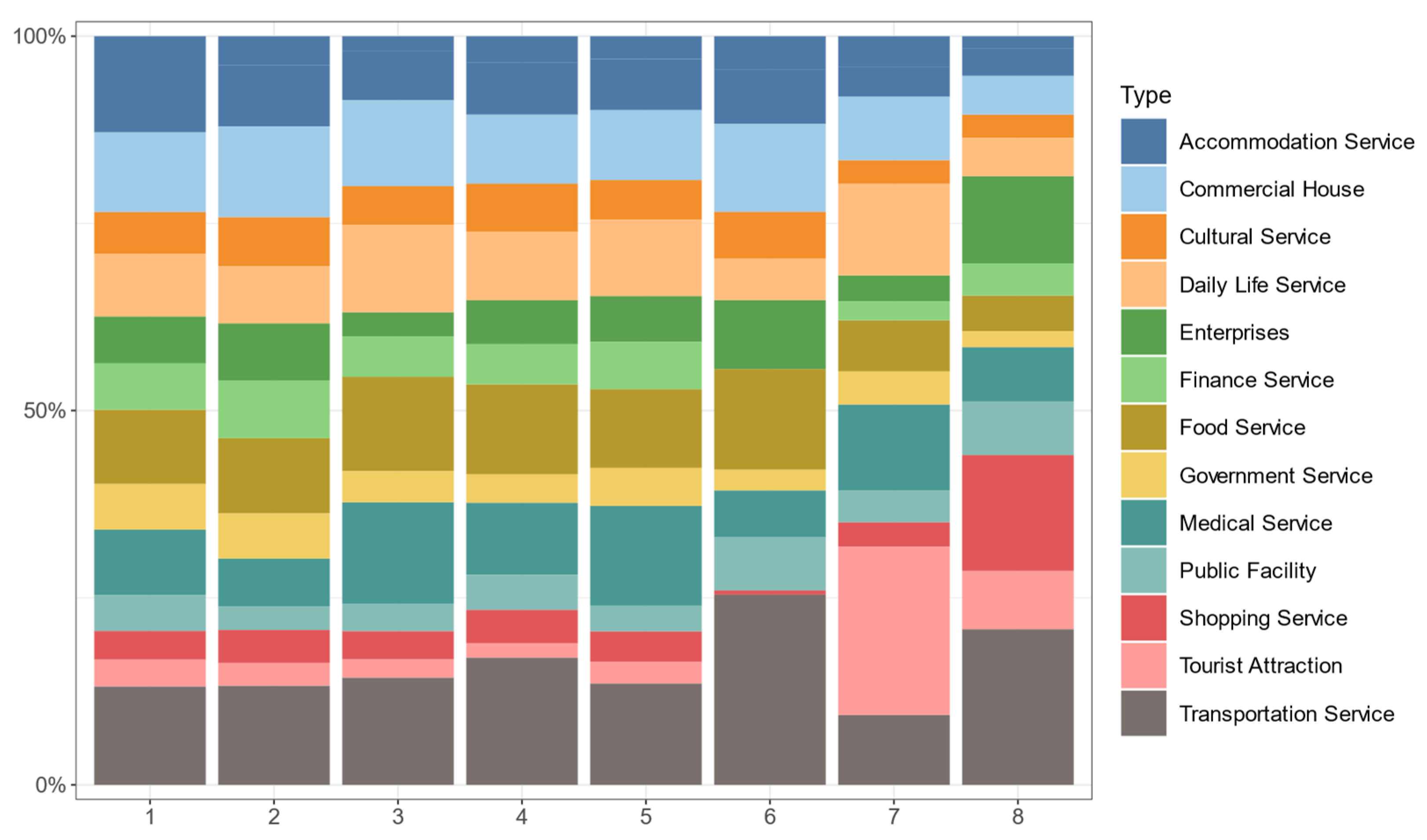
4.5. POI Analysis and Identification of Functional Zones

The spatial partitions derived based on the contribution indices of different IMF components can initially explore the spatio-temporal patterns of urban traffic flows. In order to discover the regional functional features related to each spatial clustering result, this paper combines the spatial partitioning results with the POI data in Chengdu for analysis and identification of functional areas with the actual locations.

In this study, the number of various types of POIs on each grid is counted, averaged, and standardized from 0 to 1 in turn. After that, the percentage of different types of POIs on each type of space partition is calculated, as shown in Figure 10.

Cluster 1 is the center of the research area, with a strong daily traffic rhythm but poor short-term traffic flow characteristics. Cluster 1 has many types and numbers of POIs, including a large number of accommodation services, daily life services, medical services, and other services, and also contains a large number of commercial houses and enterprises, etc. This area has the characteristics of a mature urban complex and is judged to be the central business/residential area.

Cluster 2 and Cluster 3 are distributed over a wide area in the middle of the second and third rings and are more discrete. These two clusters also have the same daily cycle of traffic, both of which contain a large number of POIs such as commercial houses, food services, transportation services, etc. Compared to Cluster 3, Cluster 2 contains a significantly larger number of enterprises, public facilities, and government services. Therefore, Cluster 2 is identified to be the mixed work/residential area. Cluster 3, on the other hand, has more medical services and daily life services, and is therefore judged to be the urban residential area.

Cluster 4 is located on one of the most important commuting roads in Chengdu and has more obvious daily and semi-daily cyclical characteristics. Cluster 4 has a rich infrastructure of food services, shopping services, cultural services, daily life services, transportation service, etc., and has many enterprises, which includes a variety of functions, and can be judged as the mixed-use area. Cluster 5 also has a high proportion of infrastructures such as daily life services and medical services, as well as a certain amount of accommodation services, commercial houses, and enterprises, so it can also be judged as the mixed-use area.

Cluster 6 is dispersed across several separate locations, and the IMF components that contribute the most are IMF 1–IMF 3, indicating that the traffic in Cluster 6 is of short period. Compared to other Clusters, Cluster 6 has the highest percentage of POIs for transportation services and public facilities, inferring that it is mainly the public facility service site (storage area).

In addition to the highest contribution of the daily cyclical IMF 6 in Cluster 7, the short cyclical IMF 1 also accounts for a relatively high percentage. In Cluster 7, there is also a dominant POI category, which is the tourist attraction. Meanwhile, considering that Cluster 7 has more POIs of daily life services and medical services, it is presumed that the area is the tourism area.

Cluster 8 is mainly located in the area near the third ring road of Chengdu, which also has obvious daily and semi-daily cyclical characteristics. Its corporate enterprises, public facilities, and transportation services serve the highest percentage and have certain tourist attractions. Hence, it is judged to be the commercial area.

This paper evaluates the functional zoning in relation to the actual location of each cluster. Cluster 1 is located closer to the downtown area and is the study area’s city center functional complex, with mature commercial areas such as Tianfu Square and Chunxi Road, which are Chengdu landmarks. Additionally, Cluster 1 has high-density communities, which allows it to correspond to the identification of the central business/residential area. Cluster 2 includes government institutions such as the Office of the CPC Sichuan Provincial Committee and the Armed Police Sichuan Provincial Headquarters, schools such as the University of Electronic Science and Technology and the Chengdu Railway Transportation Institute, and neighborhoods such as the Sunny Era, thus in line with the mixed work/residential area. In Cluster 3, communities appear in patches with corresponding facilities (parks, schools, etc.) and it is the urban residential area. Cluster 4 is mainly the area along the Second Ring Road in Chengdu, including office areas such as Southwest Jiaotong University and University of Electronic Science and Technology, transportation service facility areas such as Chengdu Railway Station, commercial areas such as Wangfujing Shopping Center and Impression City, and residential areas such as Longhu Sanqian Cheng, showing the characteristics of the mixed-use area. Cluster 5 contains many residential communities, and also has cultural and tourist attractions such as Shengxian Lake Park, Shahe Park, Chengdu Youth & Children’s Center, and other commercial areas such as Longfor Beicheng Paradise Walk, which undertake more comprehensive functions. Cluster 6 contains the train storage yard in the Erxianqiao area, the military area of the Western War Zone, and the Shahe area, corresponding to the military area, the land for external transportation facilities, and the interior of the park, which is in line with the land for public facility services. Cluster 7 contains places of tourist interest such as Chengdu Zoo, Seaside Park, and Shahe Park, showing obvious characteristics of the tourism area. Cluster 8 is distributed in the area near the Third Ring Road, including Greenland Red Star Plaza, IKEA, and Chengbei Building Materials Market, which are commercial areas.

5. Conclusions and Discussions

The contemporary urban landscape is dynamic and diverse sociocultural graffiti [49]. Extracting information and, ultimately, knowledge about urban form and function can better advance people’s understanding of urban morphology. This study investigates urban functional zoning to further understand urban spatial patterns and promote urban management. From the perspective of spatial-temporal coupling analysis, this study proposes a method of Urban Functional Zoning based on the Spatial Specificity (UFZ-SS). First, UFZ-SS applies the EEMD method to extract the specific periodic characteristics of traffic flows. The proposed average proportion method is then used to measure the contribution of IMFs to the original time series, thus illustrating the periodic specificity of traffic flows at different locations. The GMM clustering algorithm is utilized to classify all spatial units according to the period-specific measures of traffic flows at different locations to obtain spatial partitions. Finally, the percentage of POI types on different spatial partitions is calculated to verify the urban functions undertaken by different spatial areas.

This paper validates UFZ-SS with the online car-hailing traffic volume in northeast Chengdu, China. The results show that: (i) The periodic characteristics of traffic flows can be effectively extracted and analyzed by the EEMD method. The significance of signals with specific periods is highlighted by calculating the contribution, and different characteristics of cycle specificity are presented in different regions. (ii) Spatial clustering based on the measures of spatial specificity of urban traffic cycle can derive highly distinct and accurate urban zoning results, and achieve the identification of urban functional zones. Eight different spatial partitions within the study area are delineated and the urban function undertaken by them are identified based on their spatio-temporal characteristics and the POI data. (iii) The POIs on different partitions also verify that the functional zoning results are consistent with the actual situation in the study area.

This study innovatively applies dynamic and periodic characteristics to the functional zoning of cities, and there is much work to do in this area of research in the future: (i) In this study, only online car-hailing traffic data are used to identify urban functional zones. Other kinds of urban data, such as video camera data and cellphone location data, could be used to capture various time dynamic information of resident urban activities, for the identification of urban functional zones. (ii) The extracted periodic signals might be worthy of further analysis and discussion. This study uses the characterization of periodic signals to generate urban sub-zones by a clustering method. These periodic signals could be also used to explore and analyze the spatial disparity of resident urban activities in future studies. (iii) Building the unique spatial fingerprints of each location in a city, based on the periodic characteristics of urban traffic, is also our future research direction. We also hope more researchers explore the potential of the traffic flow cycle in urban spatial analysis.

References

1. Burlacu, S.; Gavrilă, A.; Popescu, I.M.; Gombos, S.P.; Vasilache, P.C. Theories and models of functional zoning in urban space. Rev. De Manag. Comp. Int. 2020, 21, 44–53. [Google Scholar]
2. Zhang, H.; Zhang, L.; Che, F.; Jia, J.; Shi, B. Revealing urban traffic demand by constructing dynamic networks with taxi trajectory data. IEEE Access 2020, 8, 147673–147681. [Google Scholar] [CrossRef]
3. Schiavina, M.; Melchiorri, M.; Freire, S.; Florio, P.; Ehrlich, D.; Tommasi, P.; Pesaresi, M.; Kemper, T. Land use efficiency of functional urban areas: Global pattern and evolution of development trajectories. Habitat Int. 2022, 123, 102543. [Google Scholar] [CrossRef] [PubMed]
4. Liu, F.; Andrienko, G.; Andrienko, N.; Chen, S.; Janssens, D.; Wets, G.; Theodoridis, Y. Citywide Traffic Analysis Based on the Combination of Visual and Analytic Approaches. J. Geovisualization Spat. Anal. 2020, 4, 15. [Google Scholar] [CrossRef]
5. Gao, S.; Liu, Y.; Wang, Y.; Ma, X. Discovering Spatial Interaction Communities from Mobile Phone Data. Trans. GIS 2013, 17, 463–481. [Google Scholar] [CrossRef] [Green Version]
6. Srivastava, S.; Vargas-Muñoz, J.E.; Swinkels, D.; Tuia, D. Multilabel building functions classification from ground pictures using convolutional neural networks. In Proceedings of the 2nd ACM SIGSPATIAL International Workshop on AI for Geographic Knowledge Discovery, Seattle, WA, USA, 6 November 2018; pp. 43–46. [Google Scholar]
7. Domingo, D.; Palka, G.; Hersperger, A.M. Effect of zoning plans on urban land-use change: A multi-scenario simulation for supporting sustainable urban growth. Sustain. Cities Soc. 2021, 69, 102833. [Google Scholar] [CrossRef]
8. Manley, E. Identifying functional urban regions within traffic flow. Reg. Stud. Reg. Sci. 2014, 1, 40–42. [Google Scholar] [CrossRef]
9. Reis, J.P.; Silva, E.A.; Pinho, P. Spatial metrics to study urban patterns in growing and shrinking cities. Urban Geogr. 2016, 37, 246–271. [Google Scholar] [CrossRef]
10. Huynh, H.N.; Makarov, E.; Legara, E.F.; Monterola, C.; Chew, L.Y. Characterisation and comparison of spatial patterns in urban systems: A case study of US cities. J. Comput. Sci. 2018, 24, 34–43. [Google Scholar] [CrossRef] [Green Version]
11. Huang, H.; Yao, X.A.; Krisp, J.M.; Jiang, B. Analytics of location-based big data for smart cities: Opportunities, challenges, and future directions. Comput. Environ. Urban Syst. 2021, 90, 101712. [Google Scholar] [CrossRef]
12. Pei, T.; Song, C.; Guo, S.; Shu, H.; Liu, Y.; Du, Y.; Ma, T.; Zhou, C. Big geodata mining: Objective, connotations and research issues. J. Geogr. Sci. 2020, 30, 251–266. [Google Scholar] [CrossRef]
13. Wu, T.; Shen, Q.; Xu, M.; Peng, T.; Ou, X. Development and application of an energy use and CO2 emissions reduction evaluation model for China’s online car hailing services. Energy 2018, 154, 298–307. [Google Scholar] [CrossRef]
14. Zhang, B.; Chen, S.; Ma, Y.; Li, T.; Tang, K. Analysis on spatiotemporal urban mobility based on online car-hailing data. J. Transp. Geogr. 2020, 82, 102568. [Google Scholar] [CrossRef]
15. Brockmann, D.; Theis, F. Money Circulation, Trackable Items, and the Emergence of Universal Human Mobility Patterns. IEEE Pervasive Comput. 2008, 7, 28–35. [Google Scholar] [CrossRef]
16. Doyle, J.; Hung, P.; Farrell, R.; McLoone, S. Population Mobility Dynamics Estimated from Mobile Telephony Data. J. Urban Technol. 2014, 21, 109–132. [Google Scholar] [CrossRef]
17. Pieroni, C.; Giannotti, M.; Alves, B.B.; Arbex, R. Big data for big issues: Revealing travel patterns of low-income population based on smart card data mining in a global south unequal city. J. Transp. Geogr. 2021, 96, 103203. [Google Scholar] [CrossRef]
18. Wolf, J.; Oliveira, M.; Thompson, M. Impact of Underreporting on Mileage and Travel Time Estimates: Results from Global Positioning System-Enhanced Household Travel Survey. Transp. Res. Rec. 2003, 1854, 189–198. [Google Scholar] [CrossRef]
19. Hu, S.; Gao, S.; Wu, L.; Xu, Y.; Zhang, Z.; Cui, H.; Gong, X. Urban function classification at road segment level using taxi trajectory data: A graph convolutional neural network approach. Comput. Environ. Urban Syst. 2021, 87, 101619. [Google Scholar] [CrossRef]
20. Bogaerts, T.; Masegosa, A.D.; Angarita-Zapata, J.S.; Onieva, E.; Hellinckx, P. A graph CNN-LSTM neural network for short and long-term traffic forecasting based on trajectory data. Transp. Res. Part C: Emerg. Technol. 2020, 112, 62–77. [Google Scholar] [CrossRef]
21. Dokuz, A.S. Weighted spatio-temporal taxi trajectory big data mining for regional traffic estimation. Phys. A Stat. Mech. Its Appl. 2022, 589, 126645. [Google Scholar] [CrossRef]
22. Loo, B.P.Y.; Huang, Z. Delineating traffic congestion zones in cities: An effective approach based on GIS. J. Transp. Geogr. 2021, 94, 103108. [Google Scholar] [CrossRef]
23. Huang, G.; Qiao, S.; Yeh, A.G.-O. Spatiotemporally heterogeneous willingness to ridesplitting and its relationship with the built environment: A case study in Chengdu, China. Transp. Res. Part C: Emerg. Technol. 2021, 133, 103425. [Google Scholar] [CrossRef]
24. Coccia, M.; Roshani, S.; Mosleh, M. Scientific Developments and New Technological Trajectories in Sensor Research. Sensors 2021, 21, 7803. [Google Scholar] [CrossRef] [PubMed]
25. Qureshi, K.; Abdullah, H. A Survey on Intelligent Transportation Systems. Middle-East J. Sci. Res. 2013, 15, 629–642. [Google Scholar] [CrossRef]
26. Raper, J.; Gartner, G.; Karimi, H.; Rizos, C. Applications of location–based services: A selected review. J. Locat. Based Serv. 2007, 1, 89–111. [Google Scholar] [CrossRef]
27. Lovelace, R.; Tennekes, M.; Carlino, D. ClockBoard: A zoning system for urban analysis. J. Spat. Inf. Sci. 2022, 24, 63–85. [Google Scholar]
28. Santos, C.; Hosseini, M.; Rulff, J.; Ferreira, N.; Wilson, L.; Miranda, F.; Silva, C.; Lage, M. A Visual Analytics System for Profiling Urban Land Use Evolution. arXiv 2021, arXiv:2112.06122. [Google Scholar]
29. Yuan, N.J.; Zheng, Y.; Xie, X.; Wang, Y.; Zheng, K.; Xiong, H. Discovering Urban Functional Zones Using Latent Activity Trajectories. IEEE Trans. Knowl. Data Eng. 2015, 27, 712–725. [Google Scholar] [CrossRef]
30. Herold, M.; Scepan, J.; Clarke, K.C. The Use of Remote Sensing and Landscape Metrics to Describe Structures and Changes in Urban Land Uses. Environ. Plan. A Econ. Space 2016, 34, 1443–1458. [Google Scholar] [CrossRef] [Green Version]
31. Gao, S.; Janowicz, K.; Couclelis, H. Extracting urban functional regions from points of interest and human activities on location-based social networks. Trans. GIS 2017, 21, 446–467. [Google Scholar] [CrossRef]
32. Crivellari, A.; Resch, B. Investigating functional consistency of mobility-related urban zones via motion-driven embedding vectors and local POI-type distributions. Comput. Urban Sci. 2022, 2, 19. [Google Scholar] [CrossRef] [PubMed]
33. Yu, Q.; Gu, Y.; Yang, S.; Zhou, M. Discovering Spatiotemporal Patterns and Urban Facilities Determinants of Cycling Activities in Beijing. J. Geovisualization Spat. Anal. 2021, 5, 16. [Google Scholar] [CrossRef]
34. Gao, F.; Li, S.; Tan, Z.; Liao, S. Visualizing the Spatiotemporal Characteristics of Dockless Bike Sharing Usage in Shenzhen, China. J. Geovisualization Spat. Anal. 2022, 6, 12. [Google Scholar] [CrossRef]
35. Zhang, X.; Xu, Y.; Tu, W.; Ratti, C. Do different datasets tell the same story about urban mobility—A comparative study of public transit and taxi usage. J. Transp. Geogr. 2018, 70, 78–90. [Google Scholar] [CrossRef]
36. Cai, L.; Xu, J.; Liu, J.; Ma, T.; Pei, T.; Zhou, C. Sensing multiple semantics of urban space from crowdsourcing positioning data. CITIES 2019, 93, 31–42. [Google Scholar] [CrossRef]
37. Ratti, C.; Frenchman, D.; Pulselli, R.M.; Williams, S. Mobile Landscapes: Using Location Data from Cell Phones for Urban Analysis. Environ. Plan. B Plan. Des. 2016, 33, 727–748. [Google Scholar] [CrossRef]
38. Peungnumsai, A.; Witayangkurn, A.; Nagai, M.; Miyazaki, H. A Taxi Zoning Analysis Using Large-Scale Probe Data: A Case Study for Metropolitan Bangkok. Rev. Socionetwork Strateg. 2018, 12, 21–45. [Google Scholar] [CrossRef]
39. Wu, Z.; Huang, N.E. Ensemble Empirical Mode Decomposition: A Noise-Assisted Data Analysis Method. Adv. Data Sci. Adapt. Anal. 2009, 1, 1–41. [Google Scholar] [CrossRef]
40. Peng, Z.K.; Tse, P.W.; Chu, F.L. A comparison study of improved Hilbert–Huang transform and wavelet transform: Application to fault diagnosis for rolling bearing. Mech. Syst. Signal Processing 2005, 19, 974–988. [Google Scholar] [CrossRef]
41. Han, Z.; Zhu, X.; Li, W. A False Component Identification Method of EMD Based on Kullback-leibler Divergence. Proc. Chin. Soc. Electr. Eng. 2012, 32, 112–117. [Google Scholar]
42. Cheng, J.; Yu, D.; Yang, Y. Research on the intrinsic mode function (IMF) criterion in EMD method. Mech. Syst. Signal Processing 2006, 20, 817–824. [Google Scholar]
43. Kotan, S.; Schependom, J.V.; Nagels, G.; Akan, A. Comparison of IMF Selection Methods in Classification of Multiple Sclerosis EEG Data. In Proceedings of the 2019 Medical Technologies Congress (TIPTEKNO), Izmir, Turkey, 3–5 October 2019; pp. 1–4. [Google Scholar]
44. Xue, S.; Tan, J.; Shi, L.; Deng, J. Rope Tension Fault Diagnosis in Hoisting Systems Based on Vibration Signals Using EEMD, Improved Permutation Entropy, and PSO-SVM. Entropy 2020, 22, 209. [Google Scholar] [CrossRef] [Green Version]
45. Song, C.; Pei, T. Research Progress in Time Series Clustering Methods Based on Characteristics. Prog. Geogr. 2012, 31, 1307–1317. [Google Scholar]
46. Imaouchen, Y.; Kedadouche, M.; Alkama, R.; Thomas, M. A Frequency-Weighted Energy Operator and complementary ensemble empirical mode decomposition for bearing fault detection. Mech. Syst. Signal Processing 2017, 82, 103–116. [Google Scholar] [CrossRef]
47. Di, L. On the Establishment of New National Geographic Grid for National Geographic Conditions Monitoring. Bull. Surv. Mapp. 2011, 12, 1–2. [Google Scholar]
48. Gu, Z.; Hübschmann, D. spiralize: An R package for visualizing data on spirals. Bioinformatics 2022, 38, 1434–1436. [Google Scholar] [CrossRef]
49. Crooks, A.; Pfoser, D.; Jenkins, A.; Croitoru, A.; Stefanidis, A.; Smith, D.; Karagiorgou, S.; Efentakis, A.; Lamprianidis, G. Crowdsourcing urban form and function. Int. J. Geogr. Inf. Sci. 2015, 29, 720–741. [Google Scholar] [CrossRef]
Figure 1. Illustration of the scenario being studied in this paper. (a) the example of the city space and trajectory data, (b) the traffic time series and periodic decomposition, (c) the calculation of the contribution of multi-periodic signals, and (d) the identification results of urban functional zones.
Ijgi 11 00435 g001
Figure 2. Flow chart of the EEMD method.
Ijgi 11 00435 g002
Figure 3. Study area and example of traffic volume time series. (a) Case study area in Chengdu, Sichuan province. (b) Traffic volume time series in grid145 and grid147.
Ijgi 11 00435 g003
Figure 4. Spiral diagrams of the time series of online car-hailing traffic in grid145 (a) and grid147 (b). (Note: Different colors in the spiral graph indicate different weeks, and the spiral chart is divided into 7 parts, each representing the day of the week. The height of the bar indicates the size of the flow).
Ijgi 11 00435 g004
Figure 5. EEMD decomposition results. (Note: The time series at the top is the original series, followed by IMF 1 to IMF 11 and the residual).
Ijgi 11 00435 g005
Figure 6. Spatial visualization of contribution. Each grid has a contribution value for each IMF component, which can be combined to construct the contribution matrix.
Ijgi 11 00435 g006
Figure 7. Variation of BIC value with the number of clusters.
Ijgi 11 00435 g007
Figure 8. Results of spatial clustering. Subplots (ae) represent the results of spatial partitioning into 4 to 8 classes, respectively.
Ijgi 11 00435 g008aIjgi 11 00435 g008b
Figure 9. Boxplots of the dominant period and contribution index of each IMF component of each cluster in the spatial partitioning results. (a) Dominant period of each IMF component. (b) Contribution index of each IMF component of each cluster.
Ijgi 11 00435 g009
Figure 10. Percentage of different types of POIs in each cluster. Each column (horizontal coordinate) represents a cluster, and its vertical coordinate represents the percentage of different POIs among all POIs in that cluster.
Ijgi 11 00435 g010