Abstract
A multi-modal corridor accommodates multiple modes of energy and transportation infrastructure within the same right-of-way. The existing literature on corridor routing in raster space often focuses on one mode with no consideration of the width. This is not a realistic assumption, especially if multiple modes are to co-exist within the same wide right-of-way. Moreover, newer routing methods that consider corridor width cannot take into account multi-modality and the arrangement of modes within a corridor. We developed two multi-modal wide-corridor routing methods using raster data. In the first method, the cost rasters of all modes are weighted and aggregated into a single composite on which a wide LCP is found. This wide LCP is then divided among the modes based on the desired arrangement. The second method uses a directed transformed graph in which the weight of each edge is calculated using different layers of cost data based on the edge direction, the desired widths and arrangement of the modes. Comparative analyses using synthetic datasets show the superior performance of the second proposed method in finding a muti-modal corridor in comparison with the first mode, and in finding a single-modal corridor when compared to the existing methods.
1. Introduction
This paper proposes two methods for finding a least-cost path (LCP) for wide multi-modal transportation corridors in raster space. A multi-modal transportation corridor contains two or more parallel transportation modes within the same right-of-way. Examples of multi-modal corridors include the Trans-European Transport Network, the Lamu Port South Sudan-Ethiopia Transport (LAPSSET) corridor, and Australia’s Callide infrastructure corridor. Finding an optimal path for a multi-modal corridor is more complicated than a single-mode narrow path. This complexity has roots in the two main characteristics of such corridors. First, a multi-modal corridor needs to be wide enough to safely accommodate all transportation modes. Second, the path has to be acceptable for all different modes even though various modes have different movement constraints and different environmental impacts.
Cost raster data along with GIS are widely used for optimal linear infrastructure routing, such as power lines, road, railways and pipelines. In raster data format, the study area is divided into a square grid, and each grid cell has a value from specific criterion and geographic position [1]. Generally, computerized routing methods integrate GIS tools and multi-criteria decision analysis (MCDA) to find an LCP in raster space. The basis of this approach is similar to the method explained by Ian McHarg in his book, Design with Nature [2]. For every criterion affecting travel cost, a monochrome shaded map is provided, with darker colors representing higher costs and lighter colors representing lower costs. These transparent maps are then overlaid and an optimal route is determined visually by going trough the lighter areas and avoiding the darker areas as much as possible [3].
In general, applying GIS LCP tools alongside MCDA techniques for optimal routing is done so in four steps. First, identifying the objectives and criteria important for project stakeholders. Second, gathering data on the important factors influencing the suitability of a path in the form of square grid cells, i.e., raster data. Third, assigning a suitability value to each cell, representing physical, environmental, and social barriers to ease travel through the cell. More suitable means less cost and less negative effects on the environment and society. The weight allocated to each cell—also called cost, friction or resistance—represents how difficult that cell is to pass through. Cost can be measured by money, time, distance, or risks [4]. MCDA methods, such as the analytical hierarchy process, are used to determine the ranking of important criteria and to weight them to create an accumulated cost raster. Integrating GIS and MCDA can be used either for designing purposes, i.e., finding alternative routes, or for evaluating routes that already exist [3]. Finally, we apply an LCP algorithm, such as [5], to the weighted grid network to find the shortest path that connects an origin to a destination [6].
2. Related Work and Gaps
Cost raster data and GIS are widely used to find LCPs for linear infrastructure such as roads [7,8,9], railways [10,11,12], power transmission lines [13,14], pipelines [15,16], and siting wildlife corridors [17,18]. Each transportation mode’s important criteria and ranking is different. Some studies in the literature identify these factors and weighting methods for a specific type of infrastructure; for example, ref. [19] presents a method for weighting and combining important factors for an arctic all-weather road. Other work focuses on improving the techniques for specific goals. For example, ref. [4] uses a multi-directional connectivity graph for considering anisotropic slope costs in road and canal routing, and [20] develop a road-planning method that incorporates bridges and tunnels by connecting non-adjacent cells in a connectivity graph. There is also work to make LCP algorithms faster, such as [21,22]. Another strand of the literature focuses on finding alternative or k-shortest paths [23,24]. Finding alternative paths is important because the criteria-weighting process is subjective and LCP algorithms are very sensitive to this process. Thus, it is reasonable to look at a set of alternatives rather than focusing on a single LCP.
There are two challenges in finding the shortest path for a wide multi-modal corridor that make this process more complex than single-mode, narrow-path routing. First, there is little extant work on finding wide corridors [25]. Second, current wide LCP-finding methods do not take into account the multi-modality of a corridor.
Most of the existing literature on routing assumes the width of the route is zero and unimportant compared to the raster cell size. This assumption is not realistic when high-resolution data with smaller cell size are available and routing a wide path (corridor) is desired. Ref. [26] is one of the earliest studies that pays attention to path width. They define the cost of a route connecting an origin to a destination as the cost of areas covered by the route. In [6], cell centers are considered nodes and each edge connecting two nodes is a rectangle with the width of w. The cost of each edge is equal to sum of the costs of the fraction of cells creating that rectangle. Using this definition, a wide path with the width of w can be found. However, using a sequence of these rectangle edges leads to gaps and overlap at turning points. As a result, significant errors occur when the width increases [27].
Ref. [27] reviews different methods for finding wide LCPs such as buffering or resampling. Generally, in the connectivity graph of any efficient method for finding a wide optimal path, with a width larger than a cell size, the weight of any edge (i.e., arc), cannot be calculated only from the cost of a single cell. In this case, the costs of neighboring cells are also important. Therefore, the cost of an edge needs to be calculated from a set of neighboring cells that create the desired width. For example, ref. [28] uses the weights of w-nodes which are sets of contiguous cells, and [27] uses weights of w by w blocks. These two methods are the most sophisticated for finding wide LCPs. Ref. [28] assumes that the width of a path is fixed in terms of number of cells, whereas [27] finds a path with a fixed width using Euclidean distance.
The second challenge is due to the multi-modal characteristic of corridors. A multi-modal corridor needs to be low-cost for all modes and the limitations and constraints of all modes should be considered in its routing. However, the importance of different criteria is not the same for various transportation modes. This variation has roots in different movement characteristics of various modes, different stakeholders participating in each mode’s routing, and the various economic, environmental, and social impacts of each mode. For example, a highway may block a wildlife migration route while a power transmission line or an underground pipeline is not a big barrier in this regard. The concept is similar with social acceptance. A highway may provide better connectivity and lower living costs and therefore be more acceptable for a local population than a pipeline with leakage or explosion risks. The criteria and the level of their importance affects the monetary cost of a path, which also varies across modes. For instance, a railway’s cost is much more sensitive to slope than pipelines or power lines are. Proximity to sand or gravel deposits and remoteness from river crossings have crucial effects on road costs, while they are not as important in power line routing. These differences in modes’ cost rasters result in different optimal paths for various modes in further steps. Therefore, the LCPs for different modes have variations in their courses.
To the best of authors’ knowledge, existing methods for finding wide LCP do not explicitly take into account the multi-modality of a corridor. To use these methods to find a multi-modal LCP, all cost rasters for different modes need to be weighted and combined to create a single cost raster for all modes. However, this aggregation leads to finding non-optimal paths partly due to imposing unnecessary constraints on all modes. In other words, these methods do not take into account the arrangement of modes within a corridor. For example, in a three-mode corridor consisting of a railway, a power line and a pipeline, the order of modes in different directions and the mode which is located between the two others is not considered in a routing process based on existing methods.
In this paper, we propose two methods for routing a multi-modal corridor. The first method adapts and modifies existing wide LCP methods to make them applicable to multi-modal corridors. However, non-optimal paths may be found by this method (explained further below). The second method has fundamental differences from existing methods, and considers the width of each mode as well as modes’ arrangement, i.e., the location of each mode with respect to others. This method, for each direction, uses multiple layers of cost rasters to calculate the weights of edges in its connectivity graph. The second proposed method developed for multi-modal corridors is also applicable to routing wide single-mode corridors. These methods are explained in the next section followed by numerical experiments using synthetic data.
3. Methodology
We propose two methods for determining the optimal routing of wide multi-modal infrastructure corridors. The first one finds a wide LCP on the accumulated cost raster (FWLA). In FWLA, firstly, all cost rasters for all modes are weighted and aggregated to create a single composite cost raster and, secondly, a wide LCP is found on this cost raster. Each of existing wide LCP methods such as the resampling method or methods explained in [27] or [28] could be used in the second part of the FWLA method to align a multi-modal corridor. Second, one can use a multi-layer transformed graph (MLTG). The MLTG method transforms the original graph, i.e., grid, to a new one and finds the LCP on it then the found path will be mapped on the original grid. In this method, the weights of edges in the connectivity graph are calculated from the cost rasters of different modes considering the direction of moves and the arrangement of modes in the corridor. Further elaborations are provided in the following sections.
3.1. Finding a Wide LCP on the Accumulated Cost Raster (FWLA)
There are two challenges in finding the LCP of a multi-modal corridor—first, finding a wide rather than a narrow path, and second, each cell located in the found wide-LCP should be suitable and have a low cost for the mode in that cell. The first challenge can be addressed by any of the existing wide LCP method; however, the second challenge cannot be solved completely. Existing wide LCP methods cannot take into account mode arrangement, i.e., the order of modes and the width of each. Thus, to make sure that each cell located in the corridor is suitable for its corresponding mode, the cell must be suitable for all modes. However, in this way, unnecessary constraints, i.e., to have low costs for all modes, will be imposed on the model and may result in non-optimal paths.
Ensuring the cells covered by the wide LCP are low-cost for all modes requires an aggregation process for all modes’ cost rasters before finding the LCP. We refer to this as creating a composite cost raster. One method of aggregation is a weighted average of all modes. For example, the proportion of the corridor width occupied by each mode can be used as the weight of that mode. The planner may have alternative ways of weighing different modes.
After this preliminary step, an LCP as wide as the multi-modal corridor is found on the composite cost raster using an existing method (e.g., Shirabe [27]). Finally, considering the desired arrangement of modes, all modes are accommodated within the corridor. The FWLA method, summarized in Figure 1, follows four steps: (i) using MCDA techniques to create a cost raster for each mode based on their important criteria, (ii) aggregating all cost rasters into one composite cost raster, (iii) finding a wide path on the composite cost raster, and (iv) locating the desired multi-modal corridor within the path found in (iii). It is notable that, in step (iii), all wide LCP techniques such as those introduced by [27,28] can be used to find a wide path on the aggregate cost surface.
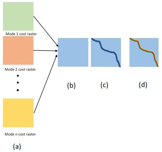
Figure 1.
Finding a Wide LCP on the accumulated cost raster (FWLA) method. Subfigure (a) shows cost rasters for n different modes. Subfigure (b) illustrates the composite cost raster created for all modes. In subfigure (c), the wide LCP on the composite cost raster is found. In subfigure (d), the desired arrangement of modes is fitted into the wide LCP found.
A shortcoming of this method is the desired arrangement of modes within the corridor is only considered in the final step and not in the wide-LCP-finding process. In other words, existing wide-LCP algorithms cannot take modes’ arrangements into account. These algorithms use the weighted average of costs regardless of the order of modes. As a result, for a cell to be considered “suitable” with a low average cost, it must be low-cost for all modes. This issue imposes unnecessary constraints on the algorithm. Figure 2 provides an illustrative example. Two synthetic cost rasters for a highway and a power line are shown in Figure 2a,b. The goal is to find a two-cell-wide path that is divided evenly among the modes and the highway is at the top of the path moving from left to right. The weights of these cost rasters are assumed to be the same and equal to . The aggregate cost raster is shown in Figure 2c; row C has a lower cost than rows A and B because both highway and power line have relatively low costs in this row. The optimal two-cell-wide path found by this method is shown in the red box in Figure 2c. However, if the average cost is not considered and the original grids are used, the optimal path would be as in Figure 2d, where the row A costs are the lowest for the highway cost raster and the row B costs are lowest for the power line cost raster. This shortcoming is solved with the proposed MLTG method, where the costs of edges are calculated based on the desired arrangements of modes in each direction; we used the MLTG method below.
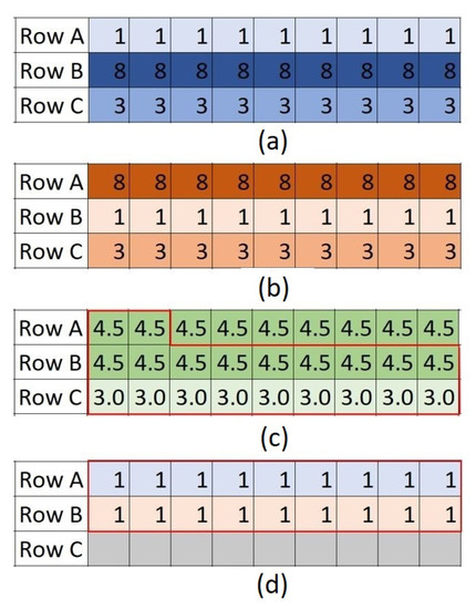
Figure 2.
Suboptimality of FWLA method with multiple modes. Subfigures (a,b) are synthetic cost rasters for a highway and a power line, respectively. Subfigure (c) shows the weighted-average cost raster for the two modes. The two-cell-wide LCP found by FWLA is highlighted in a red box in subfigure (c). The optimal two-cell-wide LCP accounting for mode-specific lowest cost is shown in Subfigure (d).
3.2. The Multi-Layer Transformed Graph (MLTG) Method
To create a wide path, the costs of a set of neighboring cells should be considered in each edge rather than the cost of only one cell. Assume that in each direction a set of cells in the shape of a rectangle as wide as the corridor is used to create a wide path and each mode based on its desired width covers a proportion of this rectangle. In connectivity graph, if each cell is connected to its eight neighboring cells, there are eight allowable directions (equivalent to the directions a queen can make in chess board). By fixing the arrangement of modes in one direction the arrangement of the other seven directions will also be fixed because the overcrossing of modes is not allowed. Therefore, the multi-modal corridor can be created by attaching rectangles that have a specific arrangement of modes for each direction. However, as discussed in Section 2, using a sequence of these rectangles edges leads to both gaps and overlaps. To overcome this challenge in the MLTG method, the original connectivity graph is transformed in a way that it does not create overlaps and it fills the gaps by adding extra costs, i.e., turning costs, where corridor changes its direction. It is notable that comparing to the conventional connectivity graph in MLTG, the nodes, edges and their weights are changed and in the next step any of LCP algorithms such as Dijkstra [5] can be used. In others words, MLTG is independent of using any algorithms for finding LCP in connectivity graphs.
MLTG builds multi-modal corridors as Legos. Each piece of Lego is in a certain color and each color represents a particular mode. Creating a continuous corridor with a desired arrangement and width for each mode requires a specific set of the Lego pieces. The cost of a corridor is the sum of the costs of the pieces creating it. Each Lego piece is built of a number of blocks and each block is made of a cell or fractions of cells in the cost rasters of modes. To calculate the weight of each Lego piece, we apply the “neighborhood” concept [29], “a set of locations that are at specified cartographic distances and/or directions from a particular location”. One particular block in each piece is considered as its reference point and the weight of each piece is calculated based on the location of its reference point and the type of neighborhood, i.e., Lego piece. At each point, the weight of each neighborhood is equal to the summation of the cost of areas occupied by different colors. For each color (mode), the cost is derived from the cost raster of that mode.
There are three types of neighborhoods in MLTG: (i) moving, (ii) clockwise turns, and (iii) counter-clockwise turns. A moving neighborhood is named based on its direction, for example, from left to right. The turning neighborhoods fill gaps created between two moving neighborhoods due to a change in direction. They are named according to the direction of the neighborhoods before and after the turning point. Table 1 shows the notation used for each neighborhood type and direction. Using the cost of a neighborhood rather than the weight of one cell allows us to find a wide LCP rather than a narrow path. Moreover, constructing the cost of a neighborhood from different cost layers allows the planner to consider the costs of all modes individually and thus avoid problems related to the use of the accumulated cost of all modes, as discussed in Section 3.1.

Table 1.
Notations used in the MLTG method for direct moves and turns.
With moves permitted in eight different directions, as the movements of queen on a chess board, eight moving neighborhoods are needed. To keep the particular arrangement of the modes, the order of modes in a reverse direction needs to be reversed. For example, the arrangement in an LR neighborhood is mirrored in RL for travel in the opposite direction. The same rule applies to clockwise and counter-clockwise turns. This concept is shown in an example 3-mode corridor in Figure 3. The required width is one cell for each of the first and third modes and two cells for the middle mode. The figure illustrates a set of moving neighborhoods and their movement directions. Several turning neighborhoods are also highlighted to show the reversed order of modes in clockwise and counter-clockwise turns.
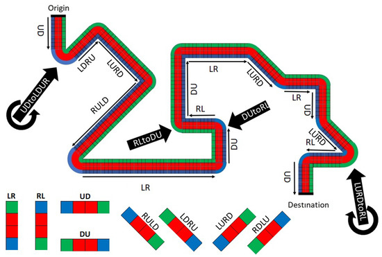
Figure 3.
An example of a 3-mode 4-cell width corridor and its eight moving neighborhoods where each mode is in a different color.
The neighborhoods can be defined such that the number of cells is consistent in each direction or in a way that the Euclidean distance of two edges of the path are consistent. Having a specified neighborhood for each direction gives flexibility to the model to have different widths in different directions. The width of each mode in each direction could be a float number. However, in this paper we make several simplifying assumptions to make the geometry simpler: (i) the corridor has a fixed width in all directions in terms of Euclidean distance, (ii) the width of each mode in orthogonal move is a factor of the cell size of cost raster, and (iii) the width of each mode in diagonal moves is a factor of . Based on these assumptions, neighborhoods are created as explained in the following paragraphs.
Consider a multi-modal corridor consisting of M modes ( where the width of the mth mode is equal to and the cell-size of the cost rasters is equal to . The required number of cells for each mode , in orthogonal moves, that create can be derived as follows:
The total width of the corridor measured by the number of cells is equal to . In Euclidean distance it is . Assume a left-to-right (LR) moving neighborhood. The origin of the Cartesian coordinate system is at the top left corner of the study area and the longitude (i) and latitude (j) increase from left to right and from top to bottom, respectively. The order of modes in LR neighborhoods from top to bottom is 1 to M with corresponding cost layers of and corresponding s of . The number of cells from the reference cell to the start of each new mode m is equal to , as per:
The cost of each neighborhood is equal to the sum of the costs of cells in that neighborhood from their corresponding cost layers. For LR neighborhoods, the reference cell is the top cell while for RL, UD, and DU the reference cells are the lowest, the leftmost, and the rightmost cells, respectively. This ensures the order of modes from the reference cell will be consistent in all moves and that the reference cell is always the beginning cell of the first mode (). A general set of eight moving neighborhoods is depicted in Figure 4. The dotted lines between the blocks mean that the number of blocks may vary in each direction. Each mode is in a different color. The first mode (blue) is the mode that includes the reference cell. The reference cell is the first block of the first mode and depicted with a black dot in the middle of the figure. The name of each neighborhood and their directions are included in the figure.
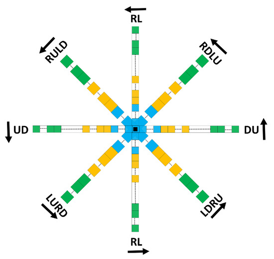
Figure 4.
The general form of eight moving neighborhoods. Each color represents a mode and the reference cell is the black square in the middle of the figure.
The general forms of LR, LRtoLURD and LURD neighborhoods, are shown in Figure 5. The input and output neighborhoods for this turn are LR and LURD, respectively. The total area of the turning neighborhood, LRtoLURD, is enclosed in a solid violet line. The cost of this turn, similar to all 16 turning neighborhoods, is equal to the area swept by its input neighborhood to reach the output neighborhood. In this case, the cost is the summation of costs of the cells enclosed by solid violet line, from different cost layers of different modes.
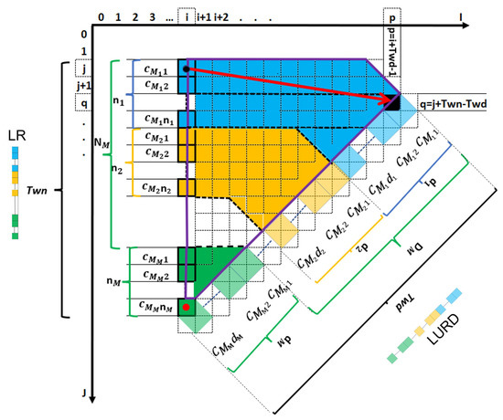
Figure 5.
Two moving neighborhoods, LR and LURD, and the turning neighborhood, LRtoLURD, which fills the gap between them are shown here. The corresponding edge related to LRtoLURD is the red arrow. The reference cell of LR at cell (i, j) and its opposite are shown by the black and red dots, respectively. The cost of each cell or block in both input and output is named in the figure. For example is the cost of the first cell of the first mode in LR. The number of cells for mode m in LR varies from 1 to while for LURD the number of blocks in mode m is between 1 and . The reference cell of LURD is located at cell .
The cost of LR neighborhood at cell is and is calculated as follows:
Equation (3) calculates the cost of the area covered by the neighborhood from the corresponding cost layers: is the cost of cell on the cost raster of mode m. It is assumed that the study area consists of I cells in width and J cells in height. Limitations of a study area need to be considered when creating the neighborhoods why the end cell of the neighborhoods are not allowed to be over the borders of the study area. The conditional term in Equation (3) ensures enough room in the study area for the corridor to move in that direction. This constraint means that at these cells the corridor does not have enough room to move in the direction of that neighborhood. For example, in a study area of 100 by 100 cells with a corridor of width 10 derived from (1), left-to-right moves are not allowable for . For the other orthogonal neighborhoods, costs can be calculated in a similar way.
Figure 6 shows a sample two-cell-width path from left-up to right-down (LURD) for the two existing sophisticated methods for wide LCPs [27,28]. In both of these methods, in diagonal directions the edges of the found path are indented with a zigzag shape. In [27], the diagonal width fluctuates by , i.e., the diameter of one cell. This issue is non-significant with a path whose width is considerably larger than the cell-size or with a smooth cost surface where there are no sharp changes in the costs of adjacent cells. However, when the width of path is not too large in terms of cell-size or when there are dramatic changes in the cost of adjacent cells the fluctuation could become more significant leading to finding a non-optimal path.
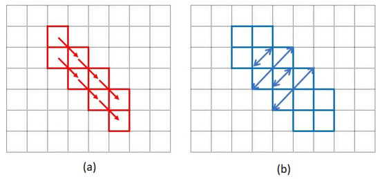
Figure 6.
The behaviours of the two existing methods for wide LCPs for a sample diagonal move in a two-cell-wide path. Subfigure (a) is a sample diagonal move when the width is constant in terms of number of cells while subfigure (b) is trying to fix the width in terms of euclidean distance.
With the MLTG method, the diagonal neighborhoods can be imagined to be constructed of a number of blocks with the same geometry. The first block consists of four half-cells, one of which is a subset of the reference cell itself. The other three half-cells are determined based on the direction of the moves. For example, in LURD neighborhoods the three other half cells are cell , cell and cell where i and j are the location of the reference cell of the neighborhood. This way, the width of each block is equal to . These blocks can be considered to have rotated 45 degrees with respect to the original grid. The concept of constructing one block using four half-cells without rotating the axis is shown in Figure 7. Figure 7b shows an LURD block consisting of four half cells from four neighboring cells. The weight of this block is equal to the summation of the four half cells shown in Figure 7a. For LDRU, RULD and RDLU neighborhoods only the location of the reference cell (black) is different. Using this method avoids indentations and fluctuations of the path width, making it possible to create a path with a constant width in diagonal moves. The constraint of being a factor of for diagonal width can be solved with more complex geometry which is beyond the scope of this paper.
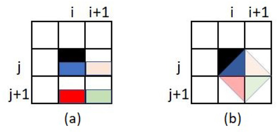
Figure 7.
Constructing a rotated block from four neighboring cells. The summation of the weights of the four half cells shown on subfigure (a) is equal to the weight of the rotated block shown in subfigure (b).
An LURD neighborhood is shown on the right side of Figure 5. For defining diagonal moves, assume that is the desired width of mode m in a multi-modal corridor. To guarantee the minimum width of , the number of blocks from each mode is calculated from Equation (7) and using (1) results in Equation (8). The order of the modes is the same as in orthogonal moves. The reference cell is one of the cells of the first block of the first mode. The total width of the corridor in diagonal moves, measured by number of blocks, is equal to:
and measured in Euclidean distance is:
The ratio ofthe width of the corridor in diagonal moves to width in orthogonal moves is:
which approaches one as the width of the corridor increases. The number of blocks from the reference cell to the first block of each mode m is and is derived from (9). The cost of an LURD neighborhood at point (i, j) is and is derived from (10), as follows. The cost of other neighborhoods is calculated in a similar way.
and if and :
Some turning neighborhoods are pointed to by black arrows in Figure 3. The gap between an existing moving neighborhood (i.e., input) and the next one (i.e., output) is filled by turning neighborhoods. Each turning neighborhood is a sector of a full circle, constructed from different layers depending on the arrangement of modes within a multi-modal corridor. To keep the arrangement fixed in all directions, the order of modes in clockwise and counter-clockwise turns are in reverse. As an example, the complete circles of turns of a three-mode corridor for both counter-clockwise and clockwise turns are shown in Figure 8a,b, respectively. In this figure, each mode is in a different color and the desired arrangement of modes in this corridor is that the black mode is on top when the corridor moves from left to right. To make the geometry simpler and calculating the weights easier in this paper, the two turning circles are modeled as two circumscribed octagons (Figure 8c,d). For each input and output moving neighborhood there is a sector in each octagon that can be used depending on the turning direction, depicted in Figure 8e,f. For each mode, if the number of blocks in its diagonal moves is equal to the number of cells in orthogonal moves, the octagon will turn into a square shape. This happens when the width of a mode is less than three cells, whereas for a wider corridor, it would be an octagon.
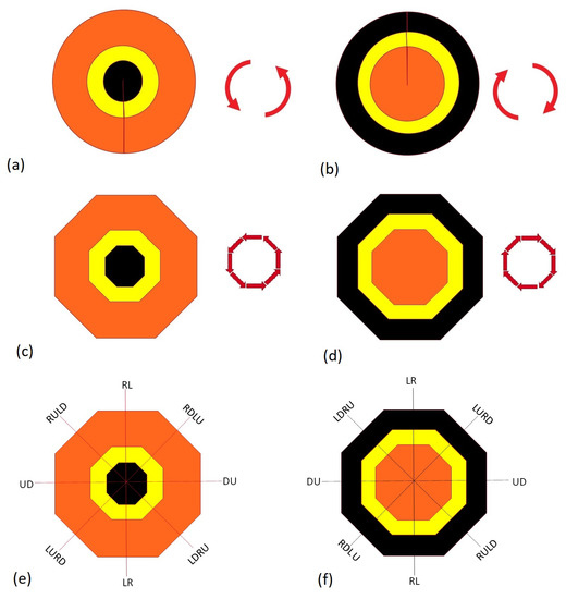
Figure 8.
The complete circles of turns for a sample three-mode corridor for both counter-clockwise and clockwise turns are shown in subfigure (a) and subfigure (b), respectively. To keep the geometry simple these circles modeled by turning octagons shown in subfigure (c) and subfigure (d). Each turn is made of an input and an output moving neighborhood which specify the sector of each turn in the turning octagons. These sectors are shown in subfigure (e) and subfigure (f) for counter-clockwise and clockwise turns, respectively.
We set several conditions to avoid even as much as half a cell of overlap. Since the turns are 45 degrees in the MLTG model, each turning neighborhood has an orthogonal and a diagonal input or output neighborhood. Half of the cost of the orthogonal neighborhood should be included in the turning neighborhood while the diagonal moves are excluded. This is because in diagonal neighborhoods are made from blocks while orthogonal neighborhoods are made from single cells- see Figure 5. In clockwise turns, the input neighborhood turns around the opposite cell of its reference cell, the red dot in Figure 5, while in counter-clockwise turns, it turns around its reference cell (black dot). In counter-clockwise turns, the reference cell of the input neighborhood needs to be eliminated from the weight of the turn. Similarly, the opposite cell of the reference cell needs to be eliminated in clockwise turns. The reason is that half of the cell is covered by the input neighborhood, here LR, and the other half is covered by the output neighborhood, here LURD. More details and equations for cost of turns are available in [30].
In conventional LCP methods, the connectivity graph consists of nodes and weighted edges. The nodes are the centers of cells in cost raster and edges are links that connect neighboring nodes. The weight of an edge is equal to the mean of costs of two connected nodes multiplied by their distance [31]. In the MLTG method, the explained conventional connectivity graph is transformed to another graph, then the LCP is found on the transformed graph, and finally the found LCP is translated to a path on the original connectivity graph.
The algorithm of [5] or other shortest-path algorithms do not differentiate between direct moves and turns. In other words, these algorithms use the nodes and weight of linking edges to find an LCP without considering whether the path is turning or is continuing in the same direction. As a solution, in the MLTG method, each cell in cost raster is considered as a graph with eight nodes corresponding to its eight possible inputs and outputs, because in the queen’s movement pattern on chessboard, each cell is surrounded by its eight neighboring cells. Each of these eight nodes works as a terminal for input and output edges (Figure 9a). The center of a cell is shown in black and each of the eight nodes is shown in a different color. Notation used for each node show the permitted moves on that node and are the same as the notations for the neighborhoods and edges shown in Table 1.
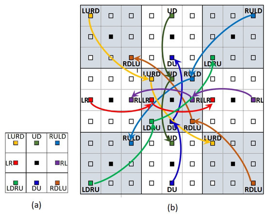
Figure 9.
One cell with its centre marked with a black square is divided into eight nodes corresponding to its eight allowable moves is shown in subfigure (a). These eight nodes are shown in different colors surrounding the black center. Eight couples of input and output direct-move edges at each cell are shown for the central cell in a -cell example in subfigure (b). The color of each couple edge is the same with the color of its corresponding node.
The cost of a path is equal to the sum of the costs of the neighborhoods creating that path, and can be calculated from Equation (11) where , and are costs of the path and costs of the moving and turning neighborhoods. In this equation, and are the total number of moving and turning neighborhoods. Therefore, in the MLTG method, the costs of neighborhoods are used as the costs of connecting edges. There are three types of edges in the MLTG method: (i) direct move edges, (ii) clockwise-turn edges, and (iii) counter-clockwise-turn edges. Each node has two direct move edges, one for each input and output. These two edges connect each node to their corresponding nodes from the two accessible cells on that direction. For example, the input direct-move edge at node LR in cell comes from the node LR of cell and the output direct-move edge goes to node LR of cell where longitude i increases from left to right. Given the eight nodes of each cell, there are eight couples of input and output direct-move edges at each cell which are shown for the central cell in a -cell example in Figure 9b.
Based on the defined geometry of neighborhoods, the weights of orthogonal moving edges are equal to the mean of the costs of two corresponding neighborhoods filling the area between those nodes and can be calculated from Equation (12). Here, is the weight of a moving edge coming from node and reaching to node where i and j show the longitude and latitude of the cell and M is the node type. is the cost of neighborhood M with its reference cell located at . For example, the weight of the LR edge connecting to is shown in Equation (13). However, the weight of diagonal moving edges and all turning edges starting from is equal to the cost of the corresponding neighborhood with its reference cell located at . The weight of diagonal moving edges and turns can be calculated from Equation (14), where is the weight of edge E starting from , and is the cost of the neighborhood E with its reference cell at .
The second type of edge is for counter-clockwise turns. In the MLTG method, there are eight nodes in each cell and for each of these nodes there are seven other nodes to turn to in a counter-clockwise direction. These seven edges are shown in Figure 10a for an LR node. Because there are eight nodes in each cell, there could be edges (Figure 10b). However, turns bigger than 45 degrees are made up of smaller 45-degree components and all these types of turns are created by connecting each node (terminal) to its neighboring node in a counter clockwise direction. This concept is depicted in Figure 10c. This way, for example, a 90-degree counter-clockwise turn from LR to DU can be created by two 45-degree turns: first from LR to LDRU, and then from LDRU to DU. The eight counter-clockwise turning edges of a cell are shown in Figure 10c.
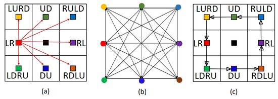
Figure 10.
(a) Eight counter-clockwise turning edges for LR. (b) 56 counter-clockwise turning edges for all eight terminals in a cell. (c) The edges in (b) can be made by the eight sequential edges shown in (c).
The third and the last type of edges is clockwise turning edges.These edges fill the gaps between the input and output neighborhoods in clockwise turns. In contrary with the counter-clockwise turns, the reference cell of input and output neighborhoods are not the same in clockwise turns. In these turns the input neighborhood turns around the opposite cell of its reference cell. Therefore both the reference cell and the terminal node are changed in clockwise turns. As an example, the red arrow in Figure 5 shows an LRtoLURD edge. The reference cell of input, i.e., LR is pointed by the black dot while the reference cell of output neighborhood, i.e., LURD is the black square.
Similar to the counter-clockwise turning edges, there are eight clockwise 45-degree turns and the larger turns can be created by adding these sequential 45 degree turns. For clockwise turns, the input neighborhood rotates around the cell on the opposite side of the reference cell. Figure 11 shows a complete cycle of clockwise turns. As an example, if the turn starts from the LR node it will go to the LURD node which is the next node in the clockwise direction. This is not the LURD node from the same cell because the output reference cell is different from the input reference cell for clockwise turns. The input reference cell and the output reference cell of an LRtoLURD turn are shown in Figure 5. As related equations show in this figure, the changes from to depend on the number of corridor cells in orthogonal and diagonal moves.
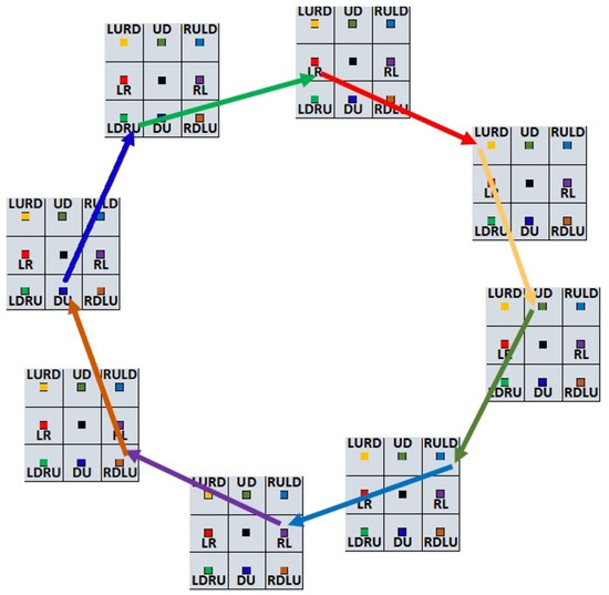
Figure 11.
Eight sequential clockwise turns for eight cells. Each node within a cell has its own cycle of clockwise turns which are not shown here to make the figure simpler. The arrows are in the same color as their starting nodes.
In summary, the MLTG model divides each cell into eight terminal nodes. Each node has three input and three output edges. Input edges include: (i) a direct edge from the counterpart node from the previous cell in that direction, (ii) a counter-clockwise turning edge from the previous node in counter-clockwise cycle in the same cell, and (iii) a clockwise turning edge from the previous node in clockwise cycle from another cell. Similarly, the three output cells are: (i) a direct edge to the counterpart node to the next cell in that direction, (ii) a counter-clockwise turning edge to the next node in counter-clockwise cycle in the same cell, and (iii) a clockwise turning edge to the next node in a clockwise cycle to another cell. These edges are shown in Figure 12.
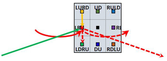
Figure 12.
Depicts the three input edges (solid lines) and the three output edges (dashed lines) for an LR node. The colors of the edges are the same as their start nodes.
4. Numerical Results
This section presents numerical simulations for finding an LCP under three scenarios. First, we compare the performance of the MLTG method with the two other existing models—[28] and [27]—in finding a two-cell-wide single-mode LCP. Although the MLTG method was created to find multi-modal wide corridors, by assigning the same cost raster to all modes, it is applicable to finding single-mode wide paths. Second, we compare the performance of the MLTG and FWLA methods in finding a multi-modal corridor. In the FWLA method, firstly a single cost-surface is created by weighting all cost-surfaces and then the [27] method is used to find a wide LCP. Last, the MLTG method is applied to find a three-mode corridor in a study area of 200 by 200 cells.
4.1. Comparing the MLTG with Existing Methods in Routing a Single-Mode Wide Corridor
Although the MLTG method is designed to find LCPs for wide multi-modal corridors, it can be used for a single-mode wide corridor. This is possible if its neighborhoods are made of a single cost raster. This section compares the performance of MLTG and two other existing methods for finding a wide single mode LCP. Specifically, we use three methods—MLTG, ref. [28], and [27]—to find a two-cell-wide single-mode LCP on a simple ten by ten cost raster. The data is synthetic and randomly made and is from [28].
First, MLTG is used to find a two-cell-wide path. Its width is fixed and equal to two cells. This is similar to the goal of the method in [28]. The moving and turning neighborhoods were so defined to keep the number of cells constant. The result is shown in Figure 13. Figure 13a is the data used as the cost layer. Figure 13b is the LCP found by [28] with aggregate cost of 31, and Figure 13c is the LCP found by the MLTG method with aggregate cost of 30. The results show the LCP found by the MLTG method for a single mode is less costly than the LCP found by [28] when the goal is to keep the number of cells constant in all transitions.
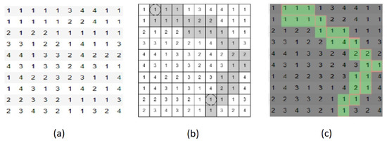
Figure 13.
(a) The cost raster values in line with [28]. (b) The single-mode two-cell-wide LCP found by [28] in grey. (c) The single-mode two-cell-wide LCP found by the MLTG method in green.
Next, we compare the MLTG and [27] methods. The data is the same as in the previous experiment and the goal is to fix the width of the LCP in terms of Euclidean distance. The result is shown in Figure 14. Subfigure (a) shows the cost values for each cell, subfigure (b) is the found MLTG LCP when the goal is to fix the Euclidean distance of two edges of the path, and subfigure (c) depicts the path on the cost values. The total cost of the MLTG method is 55. Fixing the Euclidean distance in [27] method for a two-cell-wide path means using a two by two block neighborhood. As was explained above and shown in Figure 6b, the path found by [27] cannot precisely fix the width as it fluctuates by or by one cell in terms of cell numbers. Therefore, as shown in Figure 14d, the path found by [27] in diagonal moves fluctuates by one or two cells. To make this path consistent with its goal (two-cell-width in all directions), some triangles are added wherever the width is only one cell in the diagonal moves Figure 14e. The modified path is illustrated on the cost values. To calculate the total cost of this path, half of the cost of a cell is added wherever the path occupies a triangle of a cell. The total cost of [27] is equal to 57.5 which is higher than the cost of the path found by the MLTG method (55).
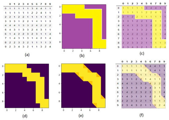
Figure 14.
(a) The cost raster values in line with [28]. (b) The single-mode two-cell-wide MLTG LCP, where the goal is to fix the Euclidean path width. (c) The path found in (b) depicted on cost-values. (d) The single-mode two-cell-wide [27] LCP. To fix the issue of the indented path found in (d), some triangles are added where the width is equal to one cell instead of two. The result is shown in (e) and it is depicted on the cost-values in (f).
4.2. Comparing the MLTG and FWLA Methods in Routing a Two-Mode Wide Corridor
Here, we compare the performance of MLTG and FWLA methods for finding the LCP for a two-mode corridor in a 10 by 10 study area. The width of each mode is one cell. In this corridor, the width is fixed in Euclidean distance and for orthogonal directions it equals . For diagonal moves, it equals . The origin of the path is at the top left corner and the destination is at the bottom right corner. We assume that one of the modes is a highway and the other is a power line, with a desired arrangement of the highway on top (north) of the power line from left to right.
The result of the FWLA method is shown in Figure 15. In this experiment, we use the [27] method to find a wide LCP on the composite cost raster. Figure 15a is the same data used in the previous experiment and it is used as the cost layer for the highway, while Figure 15b is a new data created randomly, with costs between 1 and 4 for using as the cost layer of the power line. The [27] method is designed to work on a single cost layer. To make it possible to find a two-mode corridor as described in Section 4.2 and Section 4.3, the accumulated values of all the cost layers or their average could be used. Figure 15c is the average of (a) and (b). Figure 15d shows the two-cell-wide path from the [27] approach on the average layer shown in Figure 15c. In the next step, (d) is modified into (e) to fix the issue of indented edges where the width is only one cell. In (f), the space in the corridor (e) is divided between the two modes with the desired arrangement of the corridor. However, this path is found on the average cost layer of the two modes, whereas the actual cost needs to be calculated on the original cost layers (a) and (b). In (g) the path is depicted on the highway cost layer (Figure 15a). The summation of values within the yellow area is the cost of the highway which is 27. In (h), the (f) is depicted on the cost layer of the power line, Figure 15b. The summation of values within the white area is the cost of the power line on its original cost layer which is 43. The total cost of the two modes is shown in (i) which is equal to 70.
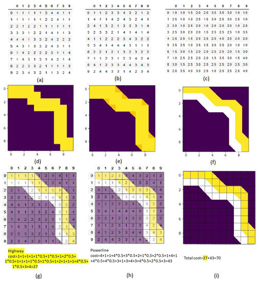
Figure 15.
Subfigure (a) is highway cost layer, using cost raster values in line with [28]). Subfigure (b) is the power line cost, data created randomly. Subfigure (c) is the average cost raster of Subfigures (a,b). Subfigure (d) is the two-cell-wide LCP method [27]. In Subfigure (e) some triangles are added to Subfigure (d) to make the width constant. In Subfigure (f), the space within Subfigure (e) is divided between two modes with the first mode in yellow and the second mode in white. In Subfigures (g,f) is overlaid on Subfigure a to calculate the cost of the highway. In Subfigures (h,f) is overlaid on Subfigure (b) to calculate the cost of the powerline. The total cost is the summation of Subfigures (g,h) that is depicted in Subfigure (i).
The same data, arrangement, widths and origin and destination as the above-mentioned example are used here to apply the MLTG method. The results are shown in Figure 16, with subfigure a displaying the found two-mode corridor. The cost of the highway, which is in yellow, is calculated in Subfigure b and is 28. The cost of the power line, illustrated in white, is shown in Subfigure c and is equal to 37. The total cost is the summation of the costs of the two modes and is 65 in total which is less than the cost of path found by FWLA (70). This shows the MLTG method found a lower cost multi-modal path.
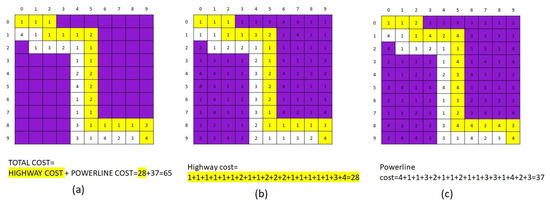
Figure 16.
The same data as in Figure 15 is used in this experiment. Subfigure (a) is a two-mode corridor found by the MLTG method with the paths of highway and power line shown in red and green, respectively. Subfigure (b) The path is depicted on the cost layer of highway and the calculated cost of highway is 28. Subfigure (c) The path is depicted on the cost layer of the powerline and the calculated cost of powerline is 37. The total cost is a summation of these two costs which is equal to 65, as shown in Subfigure (a).
4.3. The Applicability of the MLTG Method for Routing a Three-Mode Corridor in a 200 by 200 Cell Area
To check the capability of the MLTG model for a relatively larger area, a 200 by 200 cell cost raster was randomly made (Figure 17a). To make it more natural, it was smoothed twice using a 5 by 5 filter. The first and the second smoothed surfaces are shown in Figure 17b,c, respectively. In this example, we assume the data is a slope raster and is the only important criterion for routing a three-mode corridor consisting of a highway, a railway and a power transmission line, with required widths of 3, 1, and 2 cells. We further augmented the experiment by manually adding avoidance areas such as lakes, black rectangles, and rivers, white or yellow lines, to the surface. Moreover, some suitable low-cost areas are added to the area to see whether the model can distinguish them. Then, the values of the cells on this surface are classified using three different methods representing the three mentioned modes. As the sensitivities of these modes are different regarding the slope, the variability of the reclassified costs increase from the power transmission line to the highway and then to the railway. Subfigure (d) is the result of the mentioned process which is used as cost layer for the highway. Similar to Subfigure (d), Subfigure (e) is for the railway and Subfigure (f) is for the power transmission line. The resulting three-mode LCP is shown in Figure 18a, where the widths of the highway, powerline and railway are 3, 1, and 2 cells, respectively. It is notable that for finding an LCP, the MLTG model needs the origin and the destination points, and the nodes or terminals at those two points. In this example, the starting neighborhood is an LR while the destination neighborhood is a UD. Figure 18a demonstrates how the arrangement of the modes are maintained all along the path.
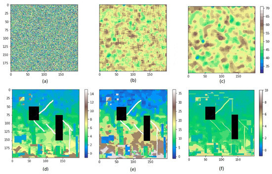
Figure 17.
Applying the MLTG method on a wide area consisting of 200 by 200 cells to find a three-mode corridor where the first mode, highway, is a three-cell-wide, the second one, railway, a two-cell-wide and the third mode, power transmission line, an only one-cell-wide path. The randomly made cost raster is shown in subfigure (a). This cost raster is smoothed two times and the results are shown in subfigures (b,c). The cells on subfigure (c) are classified using three different methods representing the three mentioned modes and some suitable areas as well as some avoidance areas are added to make it more natural. The final cost rasters for highway, railway and powerline are shown in subfigures (d–f), respectively. The black rectangles represent the added lakes which are the avoidance areas.
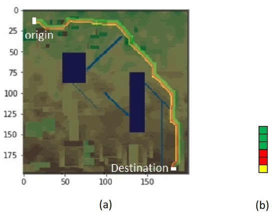
Figure 18.
Subfigure (a) shows the LCP found by the MLTG method. Subfigure (b) is the desired arrangement of an LR neighborhood of the corridor, with the highway being on top, the powerline in the middle, and the railway at the bottom.
5. Conclusions
In this paper, the two following methods for routing a multi-modal corridor are introduced. The FWLA method makes a composite cost raster of all modes, and then aligns a wide path on this cost raster using the existing methods. It accommodates all modes within the found corridor based on the desired arrangement of modes. In contrast, the MLTG method uses a transformed multi-directed graph which assigns eight nodes to each cell and connects them by specified edges. The weights of these edges are calculated based on the costs of several rotating multi-layer neighborhoods. After applying a routing algorithm, the sequence of nodes which create the multi-modal wide corridor on the transformed graph is found. These nodes are then transferred to the original grid to align the corridor.
We use numerical simulations to evaluate the performance of these methods. The results show that the MLTG method is effective in both multi-mode and single-mode wide corridor routing. The contributions made in the MLTG method is three-fold: (i) it uses multi-layer neighborhoods from different cost rasters rather than using single-layer neighborhoods from a composite cost raster; (ii) it creates the connectivity graph in a way that the gaps at the turning point are distinguished and filled by turning costs; and (iii) by using the block concept in diagonal moves, the MLTG method does not create an indented path in these directions. The numerical simulations demonstrated that the propose methods were capable of finding optimal routes while addressing the limitations imposed by the multi-modal nature of the corridors under study.
Author Contributions
Conceptualization, Mehdi Salamati, Xin Wang, Jennifer Winter and Hamidreza Zareipour; methodology, Mehdi Salamati, Xin Wang and Hamidreza Zareipour; software, Mehdi Salamati; validation, Mehdi Salamati, Xin Wang and Hamidreza Zareipour; formal analysis, Mehdi Salamati, Xin Wang and Hamidreza Zareipour; investigation, Mehdi Salamati, Xin Wang, Jennifer Winter and Hamidreza Zareipour; resources, Mehdi Salamati, Xin Wang, Jennifer Winter and Hamidreza Zareipour; data curation, Mehdi Salamati; writing—original draft preparation, Mehdi Salamati; writing—review and editing, Xin Wang, Jennifer Winter and Hamidreza Zareipour; visualization, Mehdi Salamati; supervision, Xin Wang and Hamidreza Zareipour; project administration, Jennifer Winter; funding acquisition, Jennifer Winter. All authors have read and agreed to the published version of the manuscript.
Funding
This research was funded by Social Sciences and Humanities Research Council Partnership Development Grant 890-2017-0023 PrairiesCan Grant File Number 000011411.
Conflicts of Interest
The authors declare no conflict of interest.
References
- Monteiro, C.; Ramírez-Rosado, I.J.; Miranda, V.; Zorzano-Santamaría, P.J.; García-Garrido, E.; Fernández-Jiménez, L.A. GIS spatial analysis applied to electric line routing optimization. IEEE Trans. Power Deliv. 2005, 20, 934–942. [Google Scholar] [CrossRef]
- McHarg, I.L. Design with Nature; American Museum of Natural History: New York, NY, USA, 1969. [Google Scholar]
- Jankowski, P.; Richard, L. Integration of GIS-based suitability analysis and multicriteria evaluation in a spatial decision support system for route selection. Environ. Plan. B Plan. Des. 1994, 21, 323–340. [Google Scholar] [CrossRef]
- Collischonn, W.; Pilar, J.V. A direction dependent least-cost-path algorithm for roads and canals. Int. J. Geogr. Inf. Sci. 2000, 14, 397–406. [Google Scholar] [CrossRef]
- Dijkstra, E.W. A note on two problems in connexion with graphs. Numer. Math. 1959, 1, 269–271. [Google Scholar] [CrossRef] [Green Version]
- Huber, D.L.; Church, R.L. Transmission corridor location modeling. J. Transp. Eng. 1985, 111, 114–130. [Google Scholar] [CrossRef]
- Sarı, F.; Sen, M. Least cost path algorithm design for highway route selection. Int. J. Eng. Geosci. 2017, 2, 1–8. [Google Scholar] [CrossRef] [Green Version]
- Singh, M.P.; Singh, P.; Singh, P. Fuzzy AHP-based multi-criteria decision-making analysis for route alignment planning using geographic information system (GIS). J. Geogr. Syst. 2019, 21, 395–432. [Google Scholar] [CrossRef]
- Sekulić, M.; Marinković, M.; Ivković, I. Spatial multi-criteria evaluation method for planning of optimal roads alignments, with emphasize on robustness analysis. Int. J. Traffic Transp. Eng. 2021, 11, 424–441. [Google Scholar]
- Pu, H.; Song, T.; Schonfeld, P.; Li, W.; Zhang, H.; Hu, J.; Peng, X.; Wang, J. Mountain railway alignment optimization using stepwise & hybrid particle swarm optimization incorporating genetic operators. Appl. Soft Comput. 2019, 78, 41–57. [Google Scholar]
- Yildirim, V.; Bediroglu, S. A geographic information system-based model for economical and eco-friendly high-speed railway route determination using analytic hierarchy process and least-cost-path analysis. Expert Syst. 2019, 36, e12376. [Google Scholar] [CrossRef]
- Abolhoseini, S.; Alesheikh, A.A. A new algorithm to consider critical length of grades in raster-based least-cost path analysis. Arab. J. Geosci. 2020, 13, 1032. [Google Scholar] [CrossRef]
- Bagli, S.; Geneletti, D.; Orsi, F. Routeing of power lines through least-cost path analysis and multicriteria evaluation to minimise environmental impacts. Environ. Impact Assess. Rev. 2011, 31, 234–239. [Google Scholar] [CrossRef]
- Castiglio, G.; Klas, J.; Dal Forno, M.; Resener, M. Power Line Routing Considering Aspects of Sustainable Development and Complex Environments. In Proceedings of the 2021 IEEE PES Innovative Smart Grid Technologies Conference-Latin America (ISGT Latin America), Lima, Peru, 15–17 September 2021; pp. 1–5. [Google Scholar]
- Kursah, M.B. Least-cost pipeline using geographic information system: The limit to technicalities. Int. J. Appl. Geospat. Res. (IJAGR) 2017, 8, 1–15. [Google Scholar] [CrossRef]
- Durmaz, A.I.; Ünal, E.Ö.; Aydın, C.C. Automatic pipeline route design with multi-criteria evaluation based on least-cost path analysis and line-based cartographic simplification: A case study of the mus project in Turkey. ISPRS Int. J. Geo-Inf. 2019, 8, 173. [Google Scholar] [CrossRef] [Green Version]
- Beier, P.; Majka, D.; Jenness, J. Conceptual Steps for Designing Wildlife Corridors; CorridorDesign: Flagstaff, AZ, USA, 2007. [Google Scholar]
- Li, H.; Li, D.; Li, T.; Qiao, Q.; Yang, J.; Zhang, H. Application of least-cost path model to identify a giant panda dispersal corridor network after the Wenchuan earthquake—Case study of Wolong Nature Reserve in China. Ecol. Model. 2010, 221, 944–952. [Google Scholar] [CrossRef]
- Atkinson, D.M.; Deadman, P.; Dudycha, D.; Traynor, S. Multi-criteria evaluation and least cost path analysis for an arctic all-weather road. Appl. Geogr. 2005, 25, 287–307. [Google Scholar] [CrossRef]
- Yu, C.; Lee, J.; Munro-Stasiuk, M.J. Extensions to least-cost path algorithms for roadway planning. Int. J. Geogr. Inf. Sci. 2003, 17, 361–376. [Google Scholar] [CrossRef]
- Ahuja, R.K.; Mehlhorn, K.; Orlin, J.; Tarjan, R.E. Faster algorithms for the shortest path problem. J. ACM (JACM) 1990, 37, 213–223. [Google Scholar] [CrossRef] [Green Version]
- Lefebvre, N.; Balmer, M. Fast shortest path computation in time-dependent traffic networks. Arbeitsberichte Verkehrs-Und Raumplan. 2007, 439. [Google Scholar]
- Chondrogiannis, T.; Bouros, P.; Gamper, J.; Leser, U.; Blumenthal, D.B. Finding k-shortest paths with limited overlap. VLDB J. 2020, 29, 1023–1047. [Google Scholar] [CrossRef] [Green Version]
- Thu, M. Shortest Alternative Path Finding on Road Network. In Proceedings of the 2021 IEEE 3rd Global Conference on Life Sciences and Technologies (LifeTech), Nara, Japan, 9–11 March 2021; pp. 457–460. [Google Scholar]
- Tomlin, D. Optimal Routing of Wide Corridors. In Proceedings of the Fábos Conference on Landscape and Greenway Planning, Amherst, MA, USA, 12–13 April 2013; Volume 4, p. 2. [Google Scholar]
- Newkirk, R.T. A Computer Based Planning System to Optimize Environmental Resource Allocations When Locating Utilities. Ph.D. Thesis, University of Western Ontario, London, ON, Canada, 1976. [Google Scholar]
- Shirabe, T. A method for finding a least-cost wide path in raster space. Int. J. Geogr. Inf. Sci. 2016, 30, 1469–1485. [Google Scholar] [CrossRef]
- Gonçalves, A.B. An extension of GIS-based least-cost path modelling to the location of wide paths. Int. J. Geogr. Inf. Sci. 2010, 24, 983–996. [Google Scholar] [CrossRef]
- Tomlin, C.D. Geographic Information Systems and Cartographic Modeling; Prentice-Hall: Englewood Cliffs, NJ, USA, 1990. [Google Scholar]
- Salamati, M. Optimal Routing of Multi-Modal Wide Energy and Infrastructure Corridors. Master’s Thesis, University of Calgary, Calgary, AB, Canada, 2021. [Google Scholar]
- Etherington, T.R. Least-cost modelling on irregular landscape graphs. Landsc. Ecol. 2012, 27, 957–968. [Google Scholar] [CrossRef]
Publisher’s Note: MDPI stays neutral with regard to jurisdictional claims in published maps and institutional affiliations. |
© 2022 by the authors. Licensee MDPI, Basel, Switzerland. This article is an open access article distributed under the terms and conditions of the Creative Commons Attribution (CC BY) license (https://creativecommons.org/licenses/by/4.0/).