The Influence of Data Density and Integration on Forest Canopy Cover Mapping Using Sentinel-1 and Sentinel-2 Time Series in Mediterranean Oak Forests

Abstract

Forest canopy cover (FCC) is one of the most important forest inventory parameters and plays a critical role in evaluating forest functions. This study examines the potential of integrating Sentinel-1 (S-1) and Sentinel-2 (S-2) data to map FCC in the heterogeneous Mediterranean oak forests of western Iran in different data densities (one-year datasets vs. three-year datasets). This study used very high-resolution satellite images from Google Earth, gridded points, and field inventory plots to generate a reference dataset. Based on it, four FCC classes were defined, namely non-forest, sparse forest (FCC = 1–30%), medium-density forest (FCC = 31–60%), and dense forest (FCC > 60%). In this study, three machine learning (ML) models, including Random Forest (RF), Support Vector Machine (SVM), and Classification and Regression Tree (CART), were used in the Google Earth Engine and their performance was compared for classification. Results showed that the SVM produced the highest accuracy on FCC mapping. The three-year time series increased the ability of all ML models to classify FCC classes, in particular the sparse forest class, which was not distinguished well by the one-year dataset. Class-level accuracy assessment results showed a remarkable increase in F-1 scores for sparse forest classification by integrating S-1 and S-2 (10.4% to 18.2% increased for the CART and SVM ML models, respectively). In conclusion, the synergetic use of S-1 and S-2 spectral temporal metrics improved the classification accuracy compared to that obtained using only S-2. The study relied on open data and freely available tools and can be integrated into national monitoring systems of FCC in Mediterranean oak forests of Iran and neighboring countries with similar forest attributes.

1. Introduction

Effective forest monitoring systems require novel and well-organized methods and tools to provide up-to-date, reliable data on forests [1,2]. The development of remote-sensing and image-processing techniques has enabled the automatic, cost-effective, high-quality, spatially continuous, and resource-saving mapping of forest attributes [3,4,5] across various spatial scales [6].

Forest canopy cover (FCC) is one of the most important forest inventory parameters and plays a critical role in evaluating forest functions [7,8]. For example, FCC is frequently used as an explanatory variable in water cycling [9,10,11], the assessment of soil erosion [12,13], wildlife habitat [14,15], forest regeneration and tree and forest survival [16,17], forest structure [18,19], wildfire risk assessment [20,21], and air purification [22,23]. This is because FCC reduces soil erosion by diminishing the impact of raindrops on barren surfaces [10]. Further, decreasing FCC increases understory light availability for forest regeneration [19]. Various remote-sensing techniques and data have been used for FCC mapping ever since such technologies became available [24,25,26]. Overall, FCC mapping using earth observation datasets (reference datasets) is complex due to low inter-class separability and similar spectral signatures. Moreover, large-scale FCC mapping requires sufficient numbers of training and validation samples. In previous studies, this sample was usually collected during the field inventories, which is very time-consuming and costly [27,28,29]. Therefore, enhancing FCC mapping has remained a topic of high interest for remote sensing and forestry over recent decades. Anchang et al. [30] used forest inventory plots, VHR Google Earth satellite images, and Sentinel-1 and -2 time series and reported that their methodology was able to map wood canopy cover (WCC) into 10 classes at low errors (RMSE = 8%). Arumae and Lang [31] used airborne laser scanning (ALS) data and hemispherical photography to produce an ALS-based FCC model. They also examined the influence of varying height thresholds and scan angles on FCC estimation. Based on their results, the best model was produced using all echoes and a 1.3 m height break (R² = 0.81; RMSE = 11.8%). Though previous studies have attempted to develop effective methods of using remotely sensed data, many challenges still remain regarding large-scale FCC mapping. For example, most previous studies were conducted across small sites (local scale) [32,33], and some have shown that the time series and multi-sensor image processing techniques enabled FCC mapping at higher accuracy compared to mono-date images [34,35]. However, most of them used mono-date or mono-source satellite images because they faced several limitations, such as low data storage capacity and computing power [36,37]. Further, previous FCC mapping studies were performed with cloud-free or near-cloud-free satellite imagery. They often faced low-density datasets, especially in areas with a lot of clouds.

Thanks to the advent of cloud computing platforms specialized in remote sensing, such as the Google Earth Engine (GEE), analyzing a large number of satellite images has become more effective [38,39]. The novel time series image-processing methods made it easier to integrate all cloud-free reflectance values from all images during a period and to produce spectral–temporal metrics applicable for mapping and modeling solutions [40]. Freely available satellite images, such as those obtained from the European Space Agency’s (ESA) Sentinel sensors, have been proved to be cost-effective, timely, and easy for the integration of data sources, being frequently used for FCC mapping [40,41]. The Sentinel-1 (S-1) system is composed of a constellation of two satellites that provide C-band synthetic aperture radar (SAR) data in four acquisition modes with a revisit time of 6 days [42]. Sentinel-2 (S-2) optical satellites collect high temporal resolution data, with a revisit time of 5 days, associated with a rich spectral configuration that includes 13 spectral bands [43,44]. Earlier studies reported that integrating S-1and S-2 images improved the classification accuracy of land use and land cover (LULC) classes compared to the results achieved by only S-1 or S-2 data [45,46]. The reason is that the radar signal is sensitive to the geometry (e.g., roughness, texture, and internal structure), and their physiology influences optical reflectance [47]. However, the effects of S-1 and S-2 time series integration on mapping FCC classes have not been well-studied, and there is a significant research gap in evaluating how this integration can provide better results in mapping FCC classes with a high level of spectral similarities. Although many studies have used Google Earth VHR images to prepare training and validation samples [48,49,50], they did not report the accuracy of extracted samples.

Classification algorithms are another important component, because they must produce accurate maps from remotely sensed data. An accurate and robust reference dataset is the most important component of supervised classifiers, especially machine learning (ML) models [51,52]. The field collection of reference datasets is a time-consuming and costly part of all forest monitoring studies because of the large study areas and inaccessible regions. The reference dataset should provide enough training and validation samples to represent the diversity of various canopy cover densities (including all classes of FCC) and be well distributed across the study site. When the number of training samples is not enough, there is a risk of overfitting the training data, which can lead to poor generalization capabilities of the classifier [53,54]. Providing this kind of reference dataset is challenging in large-scale FCC mapping, since training and validation samples in large area mapping are typically collected by field inventories [55]. This work builds on previous findings regarding the preparation of reliable reference datasets, novel image processing techniques, and ML models to provide a more accurate FCC map. As the upscaling artificial intelligence solutions for large-scale mapping are important, this study therefore had the following specific objectives:

(1)

Presenting a simple but efficient method for preparing an accurate reference dataset,

(2)

Evaluating the effects of data density (i.e., one-year datasets vs. three-year datasets) on FCC mapping accuracy,

(3)

Evaluating the effect of various spectral domains on FCC mapping accuracy, and

(4)

Comparing the efficiency of different ML models, namely Random Forest (RF), Support Vector Machine (SVM), and Classification and Regression Tree (CART) on FCC mapping accuracy.

2. Materials and Methods

2.1. Study Area

The study area was the Zagros Forest of the Gahvare district, which is located in Kermanshah Province, western Iran (Figure 1). The district has a total area of 940 km², a latitudinal extend from 34°25′20″ to 34°63′98″ N, and a longitudinal extend from 46°01′09″ to 46°53′67″ E (WGS84 Universal Mercator projection). Elevation ranges from 1220 to 2550 m above sea level. The study area is characterized by a Mediterranean climate, with an annual mean temperature of 22.7 °C and annual precipitation of 550 mm. Zagros forests are generally composed of sparsely treed open woodlands or shrublands dominated by oak species (Quercus sp.) [56], which are similar to the forests of other Middle Eastern countries (e.g., Iraq, Syria, Lebanon, and Turkey). The study area is dominated by coppiced Persian oak (Q. brantii Lindl.) forests. In recent decades, the region has experienced dramatic forest losses due to sudden oak death and charcoal disease, first reported in 1998 [57,58], and more recently due to the oak decline syndrome, which is a combination of climate change, diseases, and other stressors that was first observed in 2002 (see, for example, [59]).

2.2. Overall Methodology

The research methodology workflow consists of a sequence of tasks, including in situ measurements of tree crowns, the preparation of training and validation samples, accuracy assessment of reference datasets, the definition of classification datasets, and classification and accuracy assessments, as shown in Figure 2.

2.3. Reference Dataset

To prepare a sufficient number of training and validation samples, very high-resolution satellite images provided by Google Earth and visual interpretation were used. In this regard, gridded sampling points were used to measure FCC, as recommended by Anchang et al. [30]. A number of 520 square plots (40 × 40 m) were taken, corresponding to the 4 × 4 Sentinel pixels. The plot size was determined based on the tree crown attributes (such as crown perimeter) and the distribution of trees. A regular grid of sample points spaced at 4 m intervals was generated, leading to a total of 121 points per plot. The visual interpretation was used to determine the number of sample points that fell on tree crowns (green point in Figure 3). In this study, the QGis (Ver. 3.24.2) were used for creating the fishnet grid and visual interpretation. Based on the number of points overlapped on tree crowns in each plot and the total number of points located in a plot, we calculated FCC as the ratio between them.

2.4. In Situ Measurements

A field inventory to measure FCC over 70 square plots (40 × 40 m) was carried out in August 2020. The locations of all plot centers were placed using a Global Positioning System (GPS) unit; since the accuracy of GPS is affected by many factors [60], in this study, we have used a GPS unit with an accuracy of ±1 m (model: Garmin Map 64S C). Previous studies [23,61] have stated that if the tree crown followed a circular shape, the average crown diameter could be calculated by measuring two diameters of the crowns (the largest and smallest diameters of the tree crown). Therefore, horizontal tree crown projections for FCC measurement were measured using a TruPulse 360R laser range finder (Colorado, USA; https://lasertech.com/product/trupulse-360-rangefinder accessed on 1 May 2022). The average crown diameter and crown surface area were calculated based on these projections. Finally, the FCC of each plot was calculated based on Equation (1):

$$FCC=\frac{{{\displaystyle \sum }}_{i=1}^{n}CA}{PA}\times 100$$

(1)

where CA is the crown surface area, n represents the number of trees, and PA is the area of each sampling plot (i.e., 1600 m²).

2.5. Accuracy Assessment of Reference Dataset

Due to the importance of sample accuracy in efficiently training ML models, field-based FCC values were used to evaluate the accuracy of FCC values obtained by Google Earth VHR satellite images and gridded sample points. In this regard, the Pearson correlation coefficient, the coefficient of determination (R²), Root Mean Square Error (RMSE), Nash–Sutcliffe (E), and Mean Absolute Error (MAE) metrics were used to assess the relation between FCC obtained from field inventory plots and the FCC measurements based on Google Earth VHR images.

2.6. Training and Validating Samples

Four FCC classes were defined as follows: non-forest (NF), sparse forest (SF; FCC = 1–30%), medium-density forest (MDF; FCC = 31–60%), and dense forest (DF; FCC > 60%) [25,29]. Data from all 520 plots were randomly divided into training (60%) and validating (40%) subsets (

Table 1. Number of samples and pixels selected for training and validating datasets.

Forest Canopy Cover (FCC) Classes	Training Samples		Validating Samples
	No. Samples	No. Pixels	No. Samples	No. Pixels
Non-Forest (NF)	102	1632	68	1088
Sparse Forest (SF; FCC = 1–30%)	69	1104	46	736
Medium-Density Forest (MDF; FCC = 31–60%)	75	1200	50	800
Dense Forest (DF; FCC > 61%)	66	1056	44	704

). The distribution of all sample plots is represented in Figure 4.

2.7. Satellite Image Time Series and Preprocessing

Analysis of the satellite images was carried out in the GEE cloud computing platform. All S-1 synthetic aperture radar (SAR) and S-2 images were used between 1 July to 30 September 2020 ± 1 (i.e., data density = 2019, 2020, and 2021) over the study site. Data density represents the number of satellite images during a period (

Table 2. Sentinel datasets used for forest canopy cover (FCC) mapping: number of images and data density.

Sensor	Time Scale (Year)	Number of Images
S-1	2020	63
	2020 ± 1	188
S-2	2020	56
	2020 ± 1	163

). Our study site is covered by three different Sentinel tiles, including T38SND, T38SPD, and T38SPC. This limited and shortened time scale was defined to consider the stability of tree crowns. Regarding the S-2 images, all surface reflectance products with a cloud cover of less than 30% were used. The S-2 cloudless algorithm was applied for pixel-wise cloud and cloud shadow masking from the S2 image collection [62]. In terms of the S-1 time series, Ground Range Detected (GRD) dual-polarization (VV and VH) datasets in Interferometric Wide (IW) swath mode were used [63]. The efficient use of S-1 products requires some preprocessing, including applying the orbit file, thermal noise removal, terrain, radiometric correction, and speckle filtering [64]. These preprocessing operations were applied to all stored S-1 images in GEE. In this research, only the Lee filter [65] on the GEE platform with a 7×7 window was applied to reduce speckle effects, as presented in the S-1 toolbox provided in the Sentinel Application Platform (SNAP).

2.8. Auxiliary Features

In addition to S-1 and S-2 spectral bands, several vegetation indices based on S-2 visible, NIR, and red edge bands (

Table 3. Vegetation indices used in forest canopy cover (FCC) mapping.

Vegetation Index	Sentinel-2 Equation
MSAVI	$\frac{2\times \mathrm{B}8+1-\sqrt{{(2\times \mathrm{B}8+1)}^2-8\left(\mathrm{B}8-\mathrm{B}4\right)}}{2}$
DVI	$\mathrm{B}8-\mathrm{B}4$
NDVI	$\frac{\mathrm{B}8-\mathrm{B}4}{\mathrm{B}8+\mathrm{B}4}$
GNDVI	$\frac{\mathrm{B}8-\mathrm{B}3}{\mathrm{B}8+\mathrm{B}3}$
NDI45	$\frac{\mathrm{B}5-\mathrm{B}4}{\mathrm{B}5+\mathrm{B}4}$

) were calculated, including the MSAVI (Modified Soil Adjusted Vegetation Index) [66], DVI (Difference vegetation index) [67], NDVI (Normalized Difference Vegetation Index) [68], GNDVI (Green Normalized Difference Vegetation Index) [69], and NDI45 (normalized difference index based on B5 and B4) [70].

Further, the Shuttle Radar Topography Mission (SRTM) digital elevation dataset was used to extract the elevation and slope layers [71].

2.9. Sentinel Spectral–Temporal Metrics and Classification Datasets

Spectral–temporal metrics (STMs) are band-wise descriptive statistics that summarize reflectance (or an index derived thereof, such as vegetation indices) for a defined time period [72]. The S-1 and S-2 time series and auxiliary features were used to calculate STMs. For both the S-1 and S-2 time series, the same methods were used. Statistic features of the S-1 STMs, including minimum, maximum, mean, standard deviation, and 5th, 25th, 50th, 75th, and 95th percentiles for both VV and VH polarizations were calculated. For the S-2 image collection, the same statistics were calculated for all bands and vegetation indices (

Table 4. The Sentinel bands and spectral–temporal metrics (STMs) used for forest canopy cover (FCC) mapping.

Source	Bands	No. Bands	Statistical Metrics	No. STMs
S-1	VV and VH	2	Minimum, maximum, mean, standard deviation, 5th, 25th, 50th, 75th, and 95th	18
S-2	Spectral bands (B2-B8A, B11, B12) + vegetation indices (MSAVI, DVI, NDVI, GNDVI and NDI45)	15		135

). Hence, a number of 155 STMs and S-1 and S-2 spectral–temporal metrics during the peak growing season (1 July–31 September) over different time scales (2020 ± 1 and 2020) were calculated to assess the influence of data density on FCC mapping.

Finally, the impact of data density and spectral domains on the FCC mapping accuracy was evaluated. For this purpose, three datasets (

Table 5. Datasets used for forest canopy cover (FCC) mapping.

Dataset	Time Scale	Sensors	STMs
Full	2020 ± 1	S-1 and S-2	Minimum, maximum, mean, standard deviation, 5th, 25th, 50th, 75th, and 95th of all S-1 and S-2 bands + vegetation indices + elevation + slope= 155 STMs
1-year	2020	S-1 and S-2	Minimum, maximum, mean, standard deviation, 5th, 25th, 50th, 75th, and 95th of all S-1 and S-2 bands + vegetation indices + elevation + slope = 155 STMs
S2	2020 ± 1	S-2	Minimum, maximum, mean, standard deviation, 5th, 25th, 50th, 75th, and 95th of all S-2 bands + vegetation indices + elevation + slope = 137 STMs

) with different feature set configurations were defined. The results of the analysis of the full dataset (all S-1 and S-2 images between 1 July–30 September in 2020±1) and the 1-year dataset (all S-1 and S-2 images between 1 July–30 September in 2020) were compared to evaluate the impact of data density on FCC mapping. Further, regarding the influence of spectral domains and the integration of S-1 and S-2 STMs, the results of the full datasets and the S-2 dataset (only S-2 images between 1 July–30 September in 2020 ± 1) were compared.

2.10. Machine Learning Classification Models and Accuracy Assessment

Three ML models, including Random Forest (RF), Support Vector Machine (SVM), and Classification and Regression Tree (CART) were used in GEE and their performance was compared in FCC mapping. The accuracy of each classifier was tested with different combinations of parameters with a trial-and-error approach, reporting and comparing the results (

Table A1. Optimal values for the hyperparameters of the machine learning (ML) algorithms.

Dataset	ML Model	Tuning Parameter
Full	RF	ntree = 1000
	SVM	C = 5
	CART	max nodes = 10 min leaf population = 5
1-year	RF	ntree = 600
	SVM	C = 6
	CART	max nodes = 10 min leaf population = 4
S2	RF	ntree = 500
	SVM	C = 5
	CART	max nodes = 10 min leaf population = 4

).

The RF is a popular classifier that was developed based on decision trees. Its advantages are that it does not make distributional assumptions regarding the predictors, measures the importance of variables, and is less sensitive to noise or over-fitting [73]. In GEE, to maximize classification accuracy, the random forest classifier can be tuned based on several parameters, including (1) the number of decision trees, (2) the number of features per split, (3) the minimum leaf population, (4) the bag fraction, (5) the maximum number of nodes, and (6) seed randomization. In this study, we only tuned the number of decision trees and the number of predictors [5,25,74] and used the rest of the default values (https://developers.google.com/earth-engine/apidocs/ee-classifier-smilerandomforest accessed on 1 May 2022).

SVM is a kernel-based ML model that is widely used in supervised satellite image classification studies. GEE allows for setting several parameters of the model, such as (https://developers.google.com/earth-engine/apidocs/ee-classifier-libsvm accessed on 1 May 2022): the decision procedure (voting or margin), the SVM type (we used the default: C_SVC), the kernel type (linear, polynomial, sigmoid, or radial basis function), and the cost parameter (C) (how many samples within the margin contribute to the overall error) [75,76]. C is included in SVMs to estimate the associated penalty for misclassification errors [77].

The CART is a single-tree decision classifier, similar to RF [78]. At each tree node, the attribute that defines the split divides the data into subsets based on the normalized information gain. Final decisions are made based on the attribute with the highest normalized information gain [78,79]. For the CART algorithm (https://developers.google.com/earth-engine/apidocs/ee-classifier-libsvm accessed on 1 May 2022), GEE allows only two parameters to be modified: the minimum leaf population and the maximum number of nodes [80].

This study used the GEE-based hyperparameter optimizer to determine the best parameter combination that increases the learning process and further classification accuracy. In this regard, in the RF model, a number of trees were tuned. In SVM, the radial basis function (RBF) kernel type for all models was used and we only tuned the cost (C) parameter. Regarding the CART model, max nodes (the maximum number of leaf nodes in each tree) and min leaf population (minimum number of training samples in each leaf node) were tuned.

On the one hand, the performance of ML models for accurate FCC mapping was compared. On the other hand, the influence of data density on the classification performance of three ML models was assessed. Finally, the impact of combining radar (S-1) and optical (S-2) STMs was evaluated. Accuracy assessment was evaluated based on the validating samples by developing confusion matrices and exporting performance metrics, namely the overall accuracy, kappa coefficient, the Consumer’s (CA) and Producer’s (PA) accuracy, and the F-1 score. Class-level accuracy assessment metrics were calculated for a deeper analysis and better comparability between datasets. McNemar’s test was used for a better comparison of different datasets and to identify significant differences between them [81]. This test is based on a pairwise comparison of confusion matrices and expresses the chi-square (χ²) statistic as follows:

$${\chi }^2=\frac{{(f_{12}-f_{21})}^2}{f_{12}+f_{21}}$$

(2)

where f₁₂ represents the number of samples that are correctly classified by dataset-1 but wrongly classified by dataset-2, and f₂₁ represents the number of samples that are correctly classified by dataset-2 but wrongly classified by dataset-1. If the χ² is equal to or larger than 1.6 and 3.2, the differences between the two compared datasets are significant at the 95% and 99% confidence levels, respectively.

3. Results

3.1. Accuracy Assessment of Reference Dataset

Table 6. Statistics of the forest canopy cover (FCC) measurement in the field and Google Earth.

Statistics/Metrics		Field Measurement	Google Earth Measurement
Descriptive statistics	Min (%)	7.18	6.56
	Max (%)	93.59	95.94
	Mean (%)	35.29	33.49
	Median (%)	40.28	38.29
Model performance metrics	R2 (unitless)	0.9934
	RMSE (%)	2.38
	MAE (%)	2.13
	E (unitless)	0.991

shows the statistics of the FCC measured in the field and those estimated using VHR Google Earth images. Moreover, linear regression (Figure 5a and Table 6) and model performance metrics exhibited a strong relationship between the estimated FCC from Google Earth VHR images and the actual values measured in the field. The residuals showed that the differences between Google Earth FCC and field measurements range from 4.72% to 3.13% (Figure 5b). Residual plots indicated a few differences between field and Google Earth measurements of FCC.

3.2. Classification Results

The accuracy assessment results of FCC mapping are given in

Table 7. Accuracy assessment results.

Classifier	Forest Canopy Cover Classes	CA (%) *	PA (%) *	F-1 Score (%)	OA (%) *	Kappa (Unitless)
SVM	Non-Forest (NF)	96.80	97.38	97.089	91.37	0.861
	Sparse forest (SF)	85.20	63.74	72.924
	Medium-density forest (MDF)	78.89	78.02	78.453
	Dense forest (DF)	94.41	94.62	94.515
RF	Non-Forest (NF)	95.28	96.95	96.108	89.92	0.834
	Sparse forest (SF)	81.47	58.38	68.019
	Medium-density forest (MDF)	78.28	80.75	79.496
	Dense forest (DF)	91.93	91.68	91.805
CART	Non-Forest (NF)	95.29	92.44	93.844	87.22	0.794
	Sparse forest (SF)	56.17	50.38	53.1188
	Medium-density forest (MDF)	74.39	81.68	77.865
	Dense forest (DF)	93.61	89.85	91.692

* Note: CA (Consumer’s Accuracy); PA (Producer’s Accuracy); OA (Overall Accuracy).

, which is based on S-1 and S-2 STMs (full dataset) calculated during the peak growing season (1 July–31 September) over three years (2021 ± 1). Based on the results, the SVM model produced the highest accuracy (OA = 91.37% and Kappa = 0.86), and the CART model generated the lowest accuracy (OA = 87.22% and Kappa = 0.79). Further, CA, PA, and F-1 scores were higher at the class level in all classes with SVM. The lowest CA, PA, and F-1 values were produced by CART (except for CA of DF and PA of MDF). As observed in Table 7, the CA, PA, and F-1 score values for all classes (except SF) were relatively close and there were no contrasting differences between ML models. The NF class obtained the highest class level accuracy with all ML models, and CA ranged from 95.28 to 96.80%, PA ranged between 92.44 and 97.38%, and F-1 varied from 93.84 to 97.08%. The second-highest accuracy was achieved for DF (CA = 91.93–94.41%, PA = 89.85–94.62%, and F-1 score = 91.64–94.51%). For MDF class, all ML models produced a remarkable accuracy (CA = 74.39–78.89%, PA = 78.02–81.68, and F-1 = 77.45–79.49%). The lowest class level accuracy was observed for the SF, with the F-1 score ranging between 53.11 and 72.93%. These results showed that the CART model was the poorest performing model for identifying SF, whereas it performed well in classifying other FCC classes.

Based on the McNemar test (

Table 8. McNemar’s chi-squared (χ²) test with the associated probability value (p): comparison of machine learning models.

Full Dataset and S-2 Dataset	${\mathit{\chi }}^2$	p-Value
SVM vs. RF	8.69	<0.05
SVM vs. CART	32.57	<0.05
RF vs. CART	13.6	<0.05

), there were significant differences between SVM and RF ($\chi$² = 8.69), SVM and CART (χ² = 32.57), and RF and CART (χ² = 13.6) ML models. Figure 6 shows the FCC maps resulting from the ML models and full dataset.

3.3. The Influence of Data Density

Based on the results (

Table 9. Comparison of full dataset and 1-year dataset: influence of data density on forest canopy cover (FCC) mapping accuracy.

Accuracy Metric	SVM		RF		CART
	Full Dataset	1-Year Dataset	Full Dataset	1-Year Dataset	Full Dataset	1-Year Dataset
OA (%)	91.37	89.74	89.92	88.46	87.22	85.18
Avg. F-1 (%)	86.04	82.24	84.27	79.52	79.22	74.17
Kappa (unitless)	0.8612	0.8308	0.8337	0.8105	0.7942	0.7512

), all ML models produced higher accuracy with higher data density (full dataset). The OA model performance metric increased by 1.63%, 1.46%, and 2.04% with SVM, RF, and CART models when full dataset (2020±1) image collection for STM calculation was used. Among studied ML models, CART showed the highest sensitivity to data density. The Kappa coefficient and average F-1 score increased by 0.043 and 5.05%, respectively.

A comparison of FCC maps extracted from full and 1-year datasets showed a significant difference between them in all ML models (

Table 10. McNemar’s chi-squared (χ²) test with the associated probability value (p): influence of data density on forest canopy cover (FCC) mapping accuracy.

Compression	${\mathit{\chi }}^2$	p-Value
SVM_ Full vs. SVM_1-year	18.49	<0.05
RF_Full vs. RF_ 1-year	32.89	<0.05
CART_Full vs. CART_1-year	40.01	<0.05

). The largest and smallest significant difference between the two datasets was produced with the CART (CART_Full vs. CART_1-year) and SVM (SVM_ Full vs. SVM_1-year), respectively.

A high data density (i.e., full dataset) produced higher F-1 scores for all FCC classes (Figure 7). It was observed that higher data density did not have a major impact on the classification of the NF class, since the difference between the two data densities was small for all ML models. Similar results were also observed when comparing the F-1 scores between two data densities regarding MDF. Further, the results showed that the identification of SF and DF benefited the most from higher data density. The highest differences between two data densities (2020 ± 1, 2020) were observed for SF, where the F-1 score increased by 13.51%, 14.90%, and 15.18% with SVM, RF, and CART ML models, respectively. In terms of DF classification, the highest difference was observed using the SVM classifier (8.67%), closely followed by CART (7.11%) (Figure 6). In contrast, higher data density showed no remarkable increase in RF performance for DF classes (2.11%).

3.4. Influence of Spectral Domains and Integration of S-1 and S-2 STMs

Table 11. Comparison of full dataset and S-2 dataset: influence of S-1 and S-2 integration on FCC mapping accuracy.

Accuracy Metric	SVM		RF		CART
	Full Dataset	S-2 Dataset	Full Dataset	S-2 Dataset	Full Dataset	S-2 Dataset
OA (%)	91.37	89.07	89.92	86.25	87.22	86.83
Avg. F-1 (%)	86.04	85.21	84.27	79.50	79.22	78.16
Kappa (unitless)	0.8612	0.8515	0.8337	0.8054	0.7942	0.7858

shows that the classification accuracies using S-2 STMs were very high, with OA ranging between 86.83% and 89.07%. The highest accuracy was obtained using the combination of S-2 and S-1 spectral–temporal metrics (full dataset). As shown in Table 11, the synergetic use of S-1 and S-2 features showed the highest impact on RF classification results, where the OA and average F-1 scores increased by 3.67% and 4.77%, respectively. In contrast, the CART model results showed the smallest positive impact on accuracy metrics when S-1 and S-2 STMs are integrated.

When assessing differences between the full dataset and the S-2 dataset, a significant difference was only observed with the RF ML model based on the McNemar test (

Table 12. McNemar’s chi-squared (χ²) test with the associated probability value (p): influence of the integration of S-1 and S-2 on forest canopy cover (FCC) mapping accuracy.

Full Dataset and S-2 Dataset	${\mathit{\chi }}^2$	p-Value
SVM	1.34	0.2470
RF	27.89	<0.05
CART	1.55	0.2131

). The difference between the full dataset and the S-2 dataset was not significant when applying the SVM and CART ML models.

Based on class level accuracy assessment results (Figure 8), a remarkable increase in F-1 scores for the SF class was achieved by integrating S-1 and S-2 data. The F-1 score increased by 13.51%, 18.19%, and 10.44%, with SVM, RF, and CART models, respectively, when S-1 data was included in the classification. A similar result with a slight improvement was also observed for other FFC classes. For example, S-1 features improved the ability of the CART model to distinguish the DF class by 8.62%.

4. Discussion

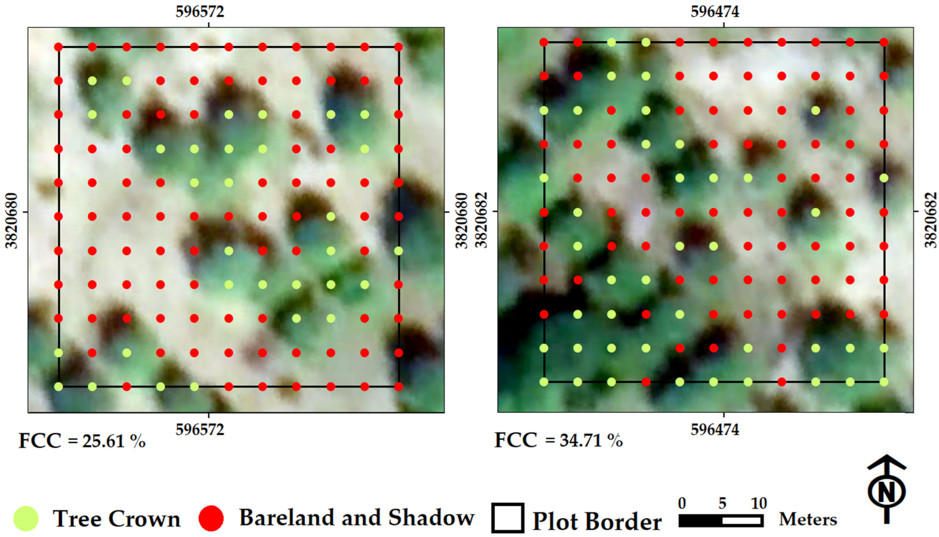
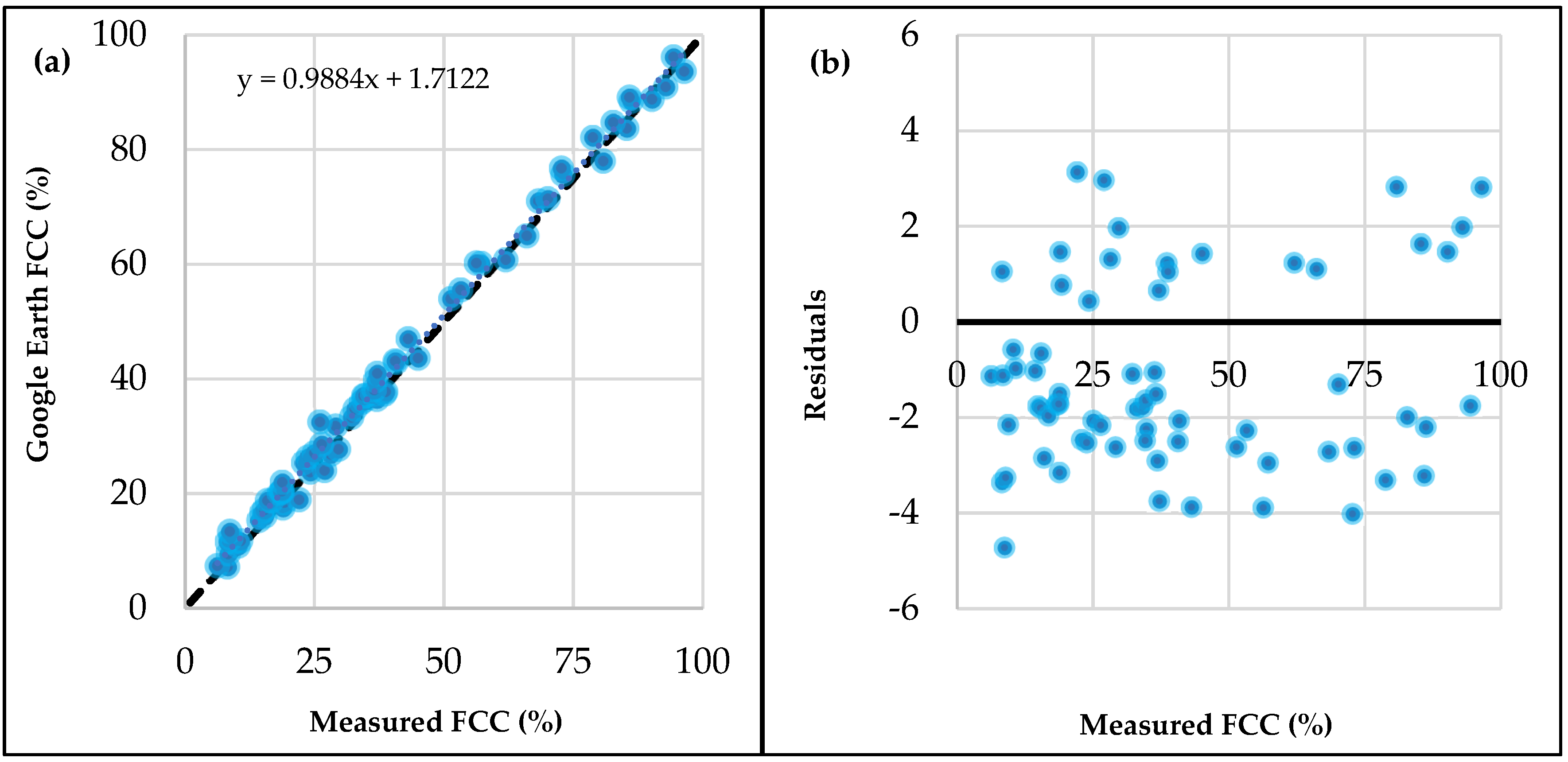
In general, combining ML models with freely available data led to satisfactory results, with the best model producing highly accurate results (OA = 91.37% and Kappa = 0.861). The first component that helped to reach these results was an accurate and robust reference dataset for FCC mapping. In this regard, VHR satellite images from Google Earth and gridded points were used to prepare 520 FCC samples, allowing us to efficiently train ML models and high-quality accuracy assessment. The accuracy of these samples was assessed based on field inventory plots, which represent the precision of the reference dataset used. In addition, a high level of correlation was observed between measured and estimated FCC values. Therefore, the present study showed that VHR satellite images provided by GEE and gridded sampling points are now a practical alternative for collecting required FCC samples fast, at a low cost. The limitations of ground-based inventories have led researchers to use various remote sensing products and methods for FCC estimation to obtain reference datasets. For example, Korhonen et al. [28] used airborne LiDAR data with a pulse density of 1/m² to estimate FCC and the resulting values as training and validating samples. Although the efficiency of using LiDAR data for providing precise forest inventory parameters has been proven in various earlier studies [82,83,84], using such data has become very costly for researchers and is constrained by technological and logistical limitations, especially in applications aiming to cover large areas, or those that require frequent applications [85,86,87]. In another study, Huang et al. [29] utilized VHR satellite images available on Google Earth to measure FCC. They defined and used a complex image processing workflow, which included taking screenshots of Google Earth images, black and white discarding, brightness and contrast adjustment, and measuring FCC using a density slice tool. They did not provide the accuracy of their measurements, and it is not possible to make a statistical comparison. Still, such complex methods require more time and more image processing experience. Hence, it was concluded that using georeferenced VHR images obtained from Google Earth for measuring FCC does not require much image processing experience and can provide a high level of accuracy.

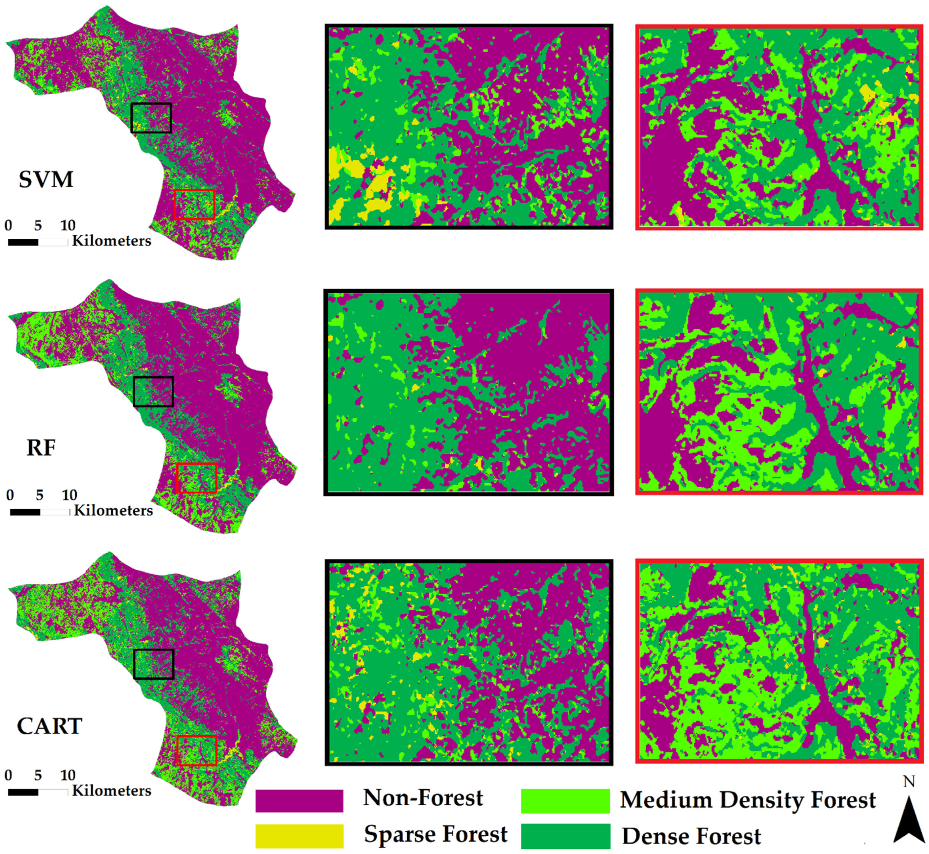
Regarding ML classifiers, the SVM produced the highest accuracy compared to RF and CART, irrespective of data density and integration. Further, based on McNemar’s test, SVM significantly outperformed RF and CART. These results are consistent with previous studies, which demonstrated that the SVM was the most efficient algorithm for LULC mapping [88,89]. The highest class level accuracy (CA, UA, and F-1 score) was produced using SVM, indicating that SVM reduces both commission and omission errors. The lowest classification accuracy was obtained using CART for all forest-covered classes. For example, the lowest F-1 scores were produced by CART for mapping sparse forest, which indicates less suitability of this algorithm for classifying features with similar spectral similarities. In the case of such similar spectral signatures, the higher ability of SVM to distinguish these classes may have been caused by its design aiming to find decision boundaries that maximize the margin [90]. In contrast, all the ML models showed similar performance for classifying other FCC classes, especially non-forest and dense forests. These results indicate that all ML models performed well when the classes were relatively pure in terms of spectral signatures, which supports previous findings. For example, based on Adugna et al. [91], RF and SVM showed similar performance for classifying pure classes with distinct spectral characteristics such as water bodies and sparse vegetation. In this study, the higher accuracy of the SVM algorithm compared to RF and CART may be related to the training sample size. Based on Shetty et al. [92], the SVM is less sensitive to the number of training samples and yields higher accuracy with a high number of features and small training samples compared to other models. Similar results were observed in other studies as well. For example, Sabat-Tomala et al. [93] compared the performance of RF and SVM algorithms in mapping three invasive species using 430 hyperspectral bands. They also evaluated the influence of training sample size on classification accuracies, for which they used different sizes of training samples (30, 50, 100, 200, and 300 samples per class). They found that SVM was more sensitive to the number of training samples than RF when many features were involved in the classification workflow. In other words, the features used for RF classification may not optimally distinguish the spectral differences between classes. Raczko and Zagajewski [94] reported that an incorrect selection of features might also affect the RF classification results. However, in some studies, RF has performed better than SVM. For example, Li et al. [95] reported that RF produced the highest OA model performance metric compared to SVM, especially for mapping complex classes such as surface-mined lands. In short, considering previous studies, RF and SVM typically showed similar abilities and often outperformed other algorithms such as CART [96], Artificial Neural Network (ANN) [97], and Maximum Likelihood Classification (MLC) [98], placing them among the best options for classification solutions.

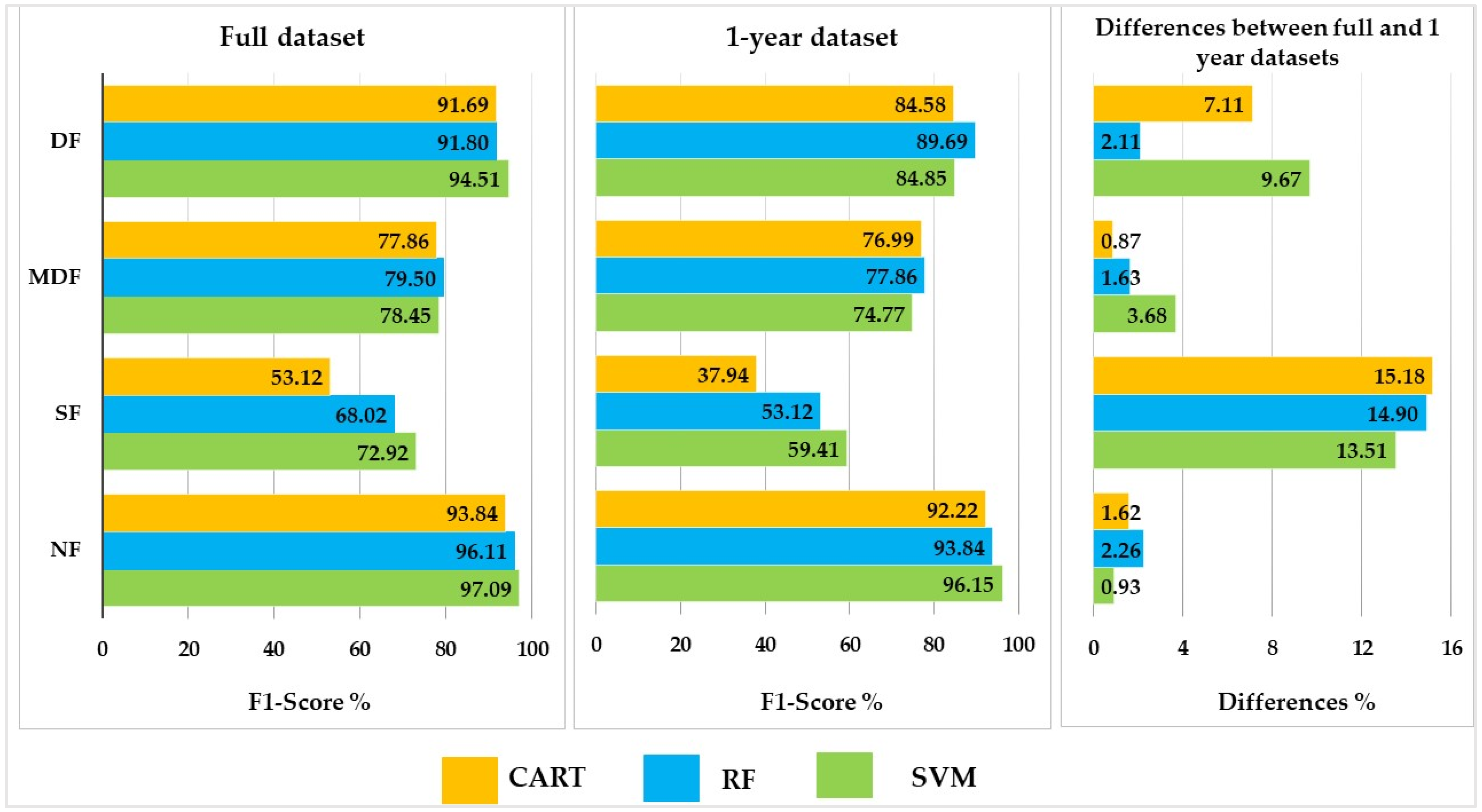
Moreover, in this study, the impact of data density on FCC classification accuracies was assessed. For example, Adams et al. [99] used all Landsat-8 OLI satellite images from 2013 to 2017, including 330 clear observations (i.e., after the cloud masking), and produced a dense time series for forest composition mapping. Azzari and Lobell [100] created a series involving all satellite images from the Landsat-7 TM, Landsat 7 ETM+, and Landsat 8 OLI sensors between 2012 and 2015 to achieve high data density and produce reliable observations for land cover monitoring in Zambia. However, in contrast to previous studies, in the current study, both one-year- and multi-year-based STMs were used to determine how high data density influenced classification results. This study observed highly significant differences associated with higher data density in all ML models. Based on the results, the OA increased by 1.63%, 1.46%, and 2.04%, respectively, with SVM, RF, and CART. The three-year time series helped all ML models and increased their ability to classify FCC classes, particularly the sparse forest class that was not distinguished well by the one-year dataset. These results are supported by Pflugmacher et al. [101], who found that the classification results increased when spectral and temporal metrics were calculated using a three-year time series instead of single-year data. Using a multi-year satellite time series is a practical and effective method for more reliably calculating STMs [102], because involving more observations can provide more information from land surface characteristics.

Regarding data integration based on results, the synergetic use of S-1 SAR and S-2 optical STMs improved the classification accuracies compared to those obtained using only S-2. The integration of S-1 STM increased the OA by 2.3%, 3.67%, and 0.39%, with SVM, RF, and CART algorithms, respectively. The integration had the highest impact on the classification of the sparse forest, which indicates that this class has similar spectral characteristics to those found in other classes, mainly non-forest and medium-density forests, and could therefore not be effectively classified by optical features. Some studies have focused on integrating optical and radar data, concluding that using them together provided better results than using them separately [103,104]. For example, Borges et al. [105] defined various feature set configurations based on S-1, S-2, and S-1 and S-2 features and stated that the synergetic use of S-1 and S-2 increased the accuracy for most land cover types. Thus, these two spectral domains provide complementary information [106].

As a first limitation, we could not conduct our study on a much larger scale due to the lack of training and validation samples. Future studies could compare the results of other popular classifiers for FCC mapping, such as ANNs and deep learning, since classification accuracy may be affected by the type of ML model used (second limitation). For instance, ANNs might work better on other classes of signals [7,107]. It was also challenging to measure the diameter of tree crowns in some sample plots due to the mountainous environment of the Zagros forests (third limitation). As a replacement option, the high-resolution images can be used to estimate the FCC for those plots located in steep areas. Further, to understand the generalizability of our approach, we would propose to test this approach such that training and testing samples would be collected from different areas, which can demonstrate the transferability of results to other regions.

At the moment, there is no official report on the FCC in the Zagros vegetation zone. Therefore, the FCC map generated using the SVM algorithm in this study could be used as a baseline for decision makers in the Forest, Rangeland, and Watershed Organization of Iran to monitor FCC changes in the region, whether they be the result of human activities or natural events, and to establish a forest management plan.

5. Conclusions

This research aimed at using all available capabilities, including VHR satellite images, field inventory plots, the Sentinel time series, GEE cloud computing, and ML algorithms to identify FCC classes in heterogeneous Mediterranean oak forests. Regarding the methodology used and the results, the following may be concluded: (i) VHR satellite images and gridded sampling points can be combined to prepare a sufficient number of training and validation samples for a fast, precise, and cost-effective approach; (ii) Sentinel optical and radar time series provide useful information for accurate FCC mapping. Their combination was the best option for identifying all FCC classes; (iii) using a three-year time series increased the ability of all ML models to classify FCC classes, mainly sparse forest that was not distinguished well using the one-year dataset. Highly significant differences associated with higher data density were observed for all ML models; (iv) the synergetic use of S-1 SAR and S-2 optical STMs improved the classification accuracies compared to those obtained using only S-2. This result emphasizes the importance of using multi-sensor datasets and different kinds of predictors in FCC mapping; (v) different ML models were examined regarding their training performance and classification accuracies based on remotely sensed datasets. Based on the results, SVM was the most efficient algorithm for FCC mapping. However, the RF also showed reasonable results. We conclude that the most popular ML models, including SVM and RF, which are provided in GEE, are sufficient for accurate FCC mapping solutions. In addition, the methodology used gives optimal and up-to-date information regarding FCC mapping and can be extended as a powerful and well-organized approach, especially in Mediterranean forests. More studies are recommended to investigate the potential of other earth observation datasets and their integration, such as Landsat and ALOS time series. Further, the performance of deep learning classifiers should be evaluated.

References

1. Jiang, H.; Song, L.; Li, Y.; Ma, M.; Fan, L. Monitoring the Reduced Resilience of Forests in Southwest China Using Long-Term Remote Sensing Data. Remote Sens. 2021, 14, 32. [Google Scholar] [CrossRef]
2. John, E.; Bunting, P.; Hardy, A.; Silayo, D.S.; Masunga, E. A Forest Monitoring System for Tanzania. Remote Sens. 2021, 13, 3081. [Google Scholar] [CrossRef]
3. Lu, Y.; Wang, L. How to Automate Timely Large-Scale Mangrove Mapping with Remote Sensing. Remote Sens. Environ. 2021, 264, 112584. [Google Scholar] [CrossRef]
4. Malkoç, E.; Rüetschi, M.; Ginzler, C.; Waser, L.T. Countrywide Mapping of Trees Outside Forests Based on Remote Sensing Data in Switzerland. Int. J. Appl. Earth Observ. Geoinf. 2021, 100, 102336. [Google Scholar] [CrossRef]
5. Moradi, F.; Darvishsefat, A.A.; Pourrahmati, M.R.; Deljouei, A.; Borz, S.A. Estimating Aboveground Biomass in Dense Hyrcanian Forests by the Use of Sentinel-2 Data. Forests 2022, 13, 104. [Google Scholar] [CrossRef]
6. White, J.C.; Coops, N.C.; Wulder, M.A.; Vastaranta, M.; Hilker, T.; Tompalski, P. Remote Sensing Technologies for Enhancing Forest Inventories: A Review. Can. J. Remote Sens. 2016, 42, 619–641. [Google Scholar] [CrossRef] [Green Version]
7. Gastón, A.; Blázquez-Cabrera, S.; Mateo-Sánchez, M.; Simón, M.; Saura, S. The Role of Forest Canopy Cover in Habitat Selection: Insights from the Iberian lynx. Eur. J. Wildl. Res. 2019, 65, 30. [Google Scholar] [CrossRef]
8. Valerio, M.; Ibáñez, R.; Gazol, A. The Role of Canopy Cover Dynamics Over a Decade of Changes in the Understory of an Atlantic Beech-Oak Forest. Forests 2021, 12, 938. [Google Scholar] [CrossRef]
9. Sadeghi, S.M.M.; Attarod, P.; Pypker, T.G. Differences in Rainfall Interception During the Growing and Non-Growing Seasons in a Fraxinus rotundifolia Plantation Located in a Semiarid Climate. J. Agric. Sci. Technol. 2015, 17, 145–156. [Google Scholar]
10. Sadeghi, S.M.M.; Gordon, D.A.; Van Stan II, J.T. A Global Synthesis of Throughfall and Stemflow Hydrometeorology. In Precipitation Partitioning by Vegetation; Springer: Berlin/Heidelberg, Germany, 2020; pp. 49–70. [Google Scholar]
11. Sadeghi, S.M.M.; Van Stan II, J.T.; Pypker, T.G.; Friesen, J. Canopy Hydrometeorological Dynamics Across a Chronosequence of a Globally Invasive Species, Ailanthus altissima (Mill., Tree of Heaven). Agric. For. Meteorol. 2017, 240, 10–17. [Google Scholar] [CrossRef]
12. Panahande, T.; Attarod, P.; Sadeghi, S.M.M.; Bayramzadeh, V.; Tang, Q.; Liu, X. The Performance of the Reformulated Gash Rainfall Interception Model in the Hyrcanian Temperate Forests of Northern Iran. J. Hydrol. 2022, 612, 128092. [Google Scholar] [CrossRef]
13. Xu, H.; Hu, X.; Guan, H.; Zhang, B.; Wang, M.; Chen, S.; Chen, M. A Remote Sensing Based Method to Detect Soil Erosion in Forests. Remote Sens. 2019, 11, 513. [Google Scholar] [CrossRef] [Green Version]
14. Hagar, J.C.; Yost, A.; Haggerty, P.K. Incorporating LiDAR Metrics Into a Structure-Based Habitat Model for a Canopy-Dwelling Species. Remote Sens. Environ. 2020, 236, 111499. [Google Scholar] [CrossRef]
15. Li, S.; Hou, Z.; Ge, J.; Wang, T. Assessing the Effects of Large Herbivores on the Three-Dimensional Structure of Temperate Forests Using Terrestrial Laser Scanning. For. Ecol. Manag. 2022, 507, 119985. [Google Scholar] [CrossRef]
16. Awasthi, N.; Aryal, K.; Chhetri, B.B.K.; Bhandari, S.K.; Khanal, Y.; Gotame, P.; Baral, K. Reflecting on Species Diversity and Regeneration Dynamics of Scientific Forest Management Practices in Nepal. For. Ecol. Manag. 2020, 474, 118378. [Google Scholar] [CrossRef]
17. Deljouei, A.; Sadeghi, S.M.M.; Abdi, E.; Bernhardt-Römermann, M.; Pascoe, E.L.; Marcantonio, M. The Impact of Road Disturbance on Vegetation and Soil Properties in a Beech Stand, Hyrcanian Forest. Eur. J. For. Res. 2018, 137, 759–770. [Google Scholar] [CrossRef]
18. Peereman, J.; Hogan, J.A.; Lin, T.C. Disturbance Frequency, Intensity and Forest Structure Modulate Cyclone-Induced Changes in Mangrove Forest Canopy Cover. Glob. Ecol. Biogeogr. 2022, 31, 37–50. [Google Scholar] [CrossRef]
19. Sefidi, K.; Copenheaver, C.A.; Sadeghi, S.M.M. Anthropogenic Pressures Decrease Structural Complexity in Caucasian forests of Iran. Écoscience 2022, 29, 199–209. [Google Scholar] [CrossRef]
20. Fernández-Álvarez, M.; Armesto, J.; Picos, J. LiDAR-Based Wildfire Prevention in WUI: The Automatic Detection, Measurement and Evaluation of Forest Fuels. Forests 2019, 10, 148. [Google Scholar] [CrossRef] [Green Version]
21. Wilson, N.; Bradstock, R.; Bedward, M. Influence of Fuel Structure Derived from Terrestrial Laser Scanning (TLS) on Wildfire Severity in Logged Forests. J. Environ. Manag. 2022, 302, 114011. [Google Scholar] [CrossRef]
22. Nowak, D.J.; Hirabayashi, S.; Doyle, M.; McGovern, M.; Pasher, J. Air Pollution Removal by Urban Forests in Canada and its Effect on Air Quality and Human Health. Urban For. Urban Green. 2018, 29, 40–48. [Google Scholar] [CrossRef]
23. Heshmatol Vaezin, S.M.; Juybari, M.M.; Daei, A.; Avatefi Hemmat, M.; Shirvany, A.; Tallis, M.J.; Hirabayashi, S.; Moeinaddini, M.; Hamidian, A.H.; Sadeghi, S.M.M. The Effectiveness of Urban Trees in Reducing Airborne Particulate Matter by Dry Deposition in Tehran, Iran. Environ. Monitor. Assess. 2021, 193, 842. [Google Scholar] [CrossRef] [PubMed]
24. Narine, L.L.; Popescu, S.; Neuenschwander, A.; Zhou, T.; Srinivasan, S.; Harbeck, K. Estimating Aboveground Biomass and Forest Canopy Cover with Simulated ICESat-2 Data. Remote Sens. Environ. 2019, 224, 1–11. [Google Scholar] [CrossRef]
25. Nasiri, V.; Darvishsefat, A.A.; Arefi, H.; Griess, V.C.; Sadeghi, S.M.M.; Borz, S.A. Modeling Forest Canopy Cover: A Synergistic Use of Sentinel-2, Aerial Photogrammetry Data, and Machine Learning. Remote Sens. 2022, 14, 1453. [Google Scholar] [CrossRef]
26. Tang, H.; Armston, J.; Hancock, S.; Marselis, S.; Goetz, S.; Dubayah, R. Characterizing Global Forest Canopy Cover Distribution Using Spaceborne Lidar. Remote Sens. Environ. 2019, 231, 111262. [Google Scholar] [CrossRef]
27. Rajabpour, M.; Darvishsefat, A.A.; Khalilpour, A. Capability of SPOT5-HRG Data for Forest Density Mapping (Case Study: Deilaman Forests in Guilan Province). Iran. J. For. Poplar Res. 2010, 18, 132–142. [Google Scholar]
28. Korhonen, L.; Ali-Sisto, D.; Tokola, T. Tropical Forest Canopy Cover Estimation Using Satellite Imagery and Airborne Lidar Reference Data. Silva Fenn. 2015, 49, 1405. [Google Scholar] [CrossRef]
29. Huang, X.; Wu, W.; Shen, T.; Xie, L.; Qin, Y.; Peng, S.; Zhou, X.; Fu, X.; Li, J.; Zhang, Z. Estimating Forest Canopy Cover by Multiscale Remote Sensing in Northeast Jiangxi, China. Land 2021, 10, 433. [Google Scholar] [CrossRef]
30. Anchang, J.Y.; Prihodko, L.; Ji, W.; Kumar, S.S.; Ross, C.W.; Yu, Q.; Lind, B.; Sarr, M.A.; Diouf, A.A.; Hanan, N.P. Toward Operational Mapping of Woody Canopy Cover in Tropical Savannas Using Google Earth Engine. Front. Environ. Sci. 2020, 8, 4. [Google Scholar] [CrossRef] [Green Version]
31. Arumäe, T.; Lang, M. Estimation of Canopy Cover in Dense Mixed-Species Forests Using Airborne Lidar Data. Eur. J. Remote Sens. 2018, 51, 132–141. [Google Scholar] [CrossRef]
32. Marsik, M.; Staub, C.G.; Kleindl, W.J.; Hall, J.M.; Fu, C.-S.; Yang, D.; Stevens, F.R.; Binford, M.W. Regional-Scale Management Maps for Forested Areas of the Southeastern United States and the US Pacific Northwest. Sci. Data 2018, 5, 180165. [Google Scholar] [CrossRef] [PubMed]
33. Myroniuk, V.; Kutia, M.; J Sarkissian, A.; Bilous, A.; Liu, S. Regional-Scale Forest Mapping Over Fragmented Landscapes Using Global Forest Products and Landsat Time Series Classification. Remote Sens. 2020, 12, 187. [Google Scholar] [CrossRef] [Green Version]
34. Desloires, J.; Ienco, D.; Botrel, A.; Ranc, N. Positive Unlabelled Learning for Satellite Images’ Time Series Analysis: An Application to Cereal and Forest Mapping. Remote Sens. 2021, 14, 140. [Google Scholar] [CrossRef]
35. Garioud, A.; Valero, S.; Giordano, S.; Mallet, C. Recurrent-Based Regression of Sentinel Time Series for Continuous Vegetation Monitoring. Remote Sens. Environ. 2021, 263, 112419. [Google Scholar] [CrossRef]
36. Liu, J.; Xue, Y.; Ren, K.; Song, J.; Windmill, C.; Merritt, P. High-Performance Time-Series Quantitative Retrieval from Satellite Images on a GPU Cluster. IEEE J. Sel. Top. Appl. Earth Obs. Remote Sens. 2019, 12, 2810–2821. [Google Scholar] [CrossRef] [Green Version]
37. Zeng, L.; Wardlow, B.D.; Xiang, D.; Hu, S.; Li, D. A Review of Vegetation Phenological Metrics Extraction Using Time-Series, Multispectral Satellite Fata. Remote Sens. Environ. 2020, 237, 111511. [Google Scholar] [CrossRef]
38. Mutanga, O.; Kumar, L. Google Earth Engine Applications. Remote Sens. 2019, 11, 591. [Google Scholar] [CrossRef] [Green Version]
39. Tamiminia, H.; Salehi, B.; Mahdianpari, M.; Quackenbush, L.; Adeli, S.; Brisco, B. Google Earth Engine for Geo-Big Data Applications: A Meta-Analysis and Systematic Review. ISPRS J. Photogramm. Remote Sens. 2020, 164, 152–170. [Google Scholar] [CrossRef]
40. Ban, Y.; Zhang, P.; Nascetti, A.; Bevington, A.R.; Wulder, M.A. Near Real-Time Wildfire Progression Monitoring with Sentinel-1 SAR Time Series and Deep Learning. Sci. Rep. 2020, 10, 1322. [Google Scholar] [CrossRef] [Green Version]
41. Jönsson, P.; Cai, Z.; Melaas, E.; Friedl, M.A.; Eklundh, L. A Method for Robust Estimation of Vegetation Seasonality from Landsat and Sentinel-2 Time Series Data. Remote Sens. 2018, 10, 635. [Google Scholar] [CrossRef] [Green Version]
42. Dostálová, A.; Lang, M.; Ivanovs, J.; Waser, L.T.; Wagner, W. European Wide Forest Classification Based on Sentinel-1 Data. Remote Sens. 2021, 13, 337. [Google Scholar] [CrossRef]
43. Moradi, F.; Sadeghi, S.M.M.; Heidarlou, H.B.; Deljouei, A.; Boshkar, E.; Borz, S.A. Above-Ground Biomass Estimation in a Mediterranean Sparse Coppice Oak Forest using Sentinel-2 Data. Ann. For. Res. 2022, 65, 165–182. [Google Scholar]
44. Phiri, D.; Simwanda, M.; Salekin, S.; Nyirenda, V.R.; Murayama, Y.; Ranagalage, M. Sentinel-2 Data for Land Cover/Use Mapping: A Review. Remote Sens. 2020, 12, 2291. [Google Scholar] [CrossRef]
45. Komisarenko, V.; Voormansik, K.; Elshawi, R.; Sakr, S. Exploiting Time Series of Sentinel-1 and Sentinel-2 to Detect Grassland Mowing Events Using Deep Learning with Reject Region. Sci. Rep. 2022, 12, 983. [Google Scholar] [CrossRef] [PubMed]
46. Mercier, A.; Betbeder, J.; Baudry, J.; Le Roux, V.; Spicher, F.; Lacoux, J.; Roger, D.; Hubert-Moy, L. Evaluation of Sentinel-1 & 2 Time Series for Predicting Wheat and Rapeseed Phenological Stages. ISPRS J. Photogramm. Remote Sens. 2020, 163, 231–256. [Google Scholar]
47. Felegari, S.; Sharifi, A.; Moravej, K.; Amin, M.; Golchin, A.; Muzirafuti, A.; Tariq, A.; Zhao, N. Integration of Sentinel 1 and Sentinel 2 Satellite Images for Crop Mapping. Appl. Sci. 2021, 11, 10104. [Google Scholar] [CrossRef]
48. Goldblatt, R.; You, W.; Hanson, G.; Khandelwal, A.K. Detecting the Boundaries of Urban Areas in India: A Dataset for Pixel-Based Image Classification in Google Earth Engine. Remote Sens. 2016, 8, 634. [Google Scholar] [CrossRef] [Green Version]
49. Magidi, J.; Nhamo, L.; Mpandeli, S.; Mabhaudhi, T. Application of the Random Forest Classifier to Map Irrigated Areas Using Google Earth Engine. Remote Sens. 2021, 13, 876. [Google Scholar] [CrossRef]
50. Pulighe, G.; Lupia, F. Mapping Spatial Patterns of Urban Agriculture in Rome (Italy) Using Google Earth and Web-Mapping Services. Land Use Policy 2016, 59, 49–58. [Google Scholar] [CrossRef]
51. Khanal, S.; Fulton, J.; Klopfenstein, A.; Douridas, N.; Shearer, S. Integration of High Resolution Remotely Sensed Data and Machine Learning Techniques for Spatial Prediction of Soil Properties and Corn Yield. Comput. Electron. Agric. 2018, 153, 213–225. [Google Scholar] [CrossRef]
52. Ramezan, C.; Warner, T.; Maxwell, A. Evaluation of Sampling and Cross-Validation Tuning Strategies for Regional-Scale Machine Learning Classification. Remote Sens. 2019, 11, 185. [Google Scholar] [CrossRef] [Green Version]
53. Chi, M.; Feng, R.; Bruzzone, L. Classification of Hyperspectral Remote-Sensing Data with Primal SVM for Small-Sized Training Dataset Problem. Adv. Space Res. 2008, 41, 1793–1799. [Google Scholar] [CrossRef]
54. Ganz, S.; Adler, P.; Kändler, G. Forest Cover Mapping Based on a Combination of Aerial Images and Sentinel-2 Satellite Data Compared to National Forest Inventory Data. Forests 2020, 11, 1322. [Google Scholar] [CrossRef]
55. Zhang, X.; Long, T.; He, G.; Guo, Y.; Yin, R.; Zhang, Z.; Xiao, H.; Li, M.; Cheng, B. Rapid Generation of Global Forest Cover Map Using Landsat Based on the Forest Ecological Zones. J. Appl. Remote Sens. 2020, 14, 022211. [Google Scholar] [CrossRef]
56. Mirhashemi, H.; Moradi, F.; Pourbabaei, H.; Mezbani, A. Changes in Flora, Life Forms and Geographical Distribution of Herbaceous Plant Species Along an Altitudinal Gradient in Oak Forests, Iran. Casp. J. Environ. Sci. 2021, 19, 619–627. [Google Scholar]
57. Attarod, P.; Rostami, F.; Dolatshahi, A.; Sadeghi, S.M.M.; Zahedi Amiri, G.; Bayramzadeh, V. Do Changes in Meteorological Parameters and Evapotranspiration Affect Declining Oak Forests of Iran? J. For. Sci. 2016, 62, 553–561. [Google Scholar] [CrossRef] [Green Version]
58. Fathizadeh, O.; Sadeghi, S.M.M.; Pazhouhan, I.; Ghanbari, S.; Attarod, P.; Su, L. Spatial Variability and Optimal Number of Rain Gauges for Sampling Throughfall Under Single Oak Trees During the Leafless Period. Forests 2021, 12, 585. [Google Scholar] [CrossRef]
59. Attarod, P.; Sadeghi, S.M.M.; Pypker, T.; Bayramzadeh, V. Oak Trees Decline; A Sign of Climate Variability Impacts in the West of Iran. Casp. J. Environ. Sci. 2017, 15, 373–384. [Google Scholar]
60. Abdi, E.; Soofi Mariv, H.; Mashayekhi, Z.; Deljouei, A.; Rahbarisisakht, S. Seasonal Variation of GPS Accuracy and Precision in Forest Road Mapping. Bull. Transilv. Uni. Bras. Ser. II For. Wood Indus Agric. Food Eng. 2022, 15, 1–12. [Google Scholar] [CrossRef]
61. Fathizadeh, O.; Sadeghi, S.M.M.; Holder, C.D.; Su, L. Leaf Phenology Drives Spatio-Temporal Patterns of Throughfall under a Single Quercus castaneifolia C.A.Mey. Forests 2020, 11, 688. [Google Scholar] [CrossRef]
62. Main-Knorn, M.; Pflug, B.; Louis, J.; Debaecker, V.; Müller-Wilm, U.; Gascon, F. Sen2Cor for Sentinel-2. In Proceedings of the Image and Signal Processing for Remote Sensing XXIII, Warsaw, Poland, 1–13 September 2017; p. 1042704. [Google Scholar]
63. Tavus, B.; Kocaman, S.; Nefeslioglu, H.; Gokceoglu, C. A Fusion Approach for Flood Mapping Using Sentinel-1 and Sentinel-2 Datasets. Int. Arch. Photogramm. Remote Sens. Spat. Inf. Sci. 2020, 43, 641–648. [Google Scholar] [CrossRef]
64. Filipponi, F. Sentinel-1 GRD Preprocessing Workflow. Proceedings 2019, 18, 11. [Google Scholar]
65. Lee, J.-S.; Jurkevich, L.; Dewaele, P.; Wambacq, P.; Oosterlinck, A. Speckle Filtering of Synthetic Aperture Radar Images: A review. Remote Sens. Rev. 1994, 8, 313–340. [Google Scholar] [CrossRef]
66. Huete, A.R. A Soil-Adjusted Vegetation Index (SAVI). Remote Sens. Environ. 1988, 25, 295–309. [Google Scholar] [CrossRef]
67. Perry, C.R., Jr.; Lautenschlager, L.F. Functional Equivalence of Spectral Vegetation Indices. Remote Sens. Environ. 1984, 14, 169–182. [Google Scholar] [CrossRef]
68. Sobhani, P.; Esmaeilzadeh, H.; Barghjelveh, S.; Sadeghi, S.M.M.; Marcu, M.V. Habitat Integrity in Protected Areas Threatened by LULC Changes and Fragmentation: A Case Study in Tehran Province, Iran. Land 2022, 11, 6. [Google Scholar] [CrossRef]
69. Gitelson, A.A.; Merzlyak, M.N. Signature Analysis of Leaf Reflectance Spectra: Algorithm Fevelopment for Remote Sensing of Chlorophyll. J. Plant Physiol. 1996, 148, 494–500. [Google Scholar] [CrossRef]
70. Delegido, J.; Verrelst, J.; Alonso, L.; Moreno, J. Evaluation of Sentinel-2 Red-Edge Bands for Empirical Estimation of Green LAI and Chlorophyll Content. Sensors 2011, 11, 7063–7081. [Google Scholar] [CrossRef] [Green Version]
71. Falorni, G.; Teles, V.; Vivoni, E.R.; Bras, R.L.; Amaratunga, K.S. Analysis and Characterization of the Vertical Accuracy of Digital Elevation Models from the Shuttle Radar Topography Mission. J. Geophys. Res. Earth Surf. 2005, 110, 1–20. [Google Scholar] [CrossRef]
72. Schug, F.; Frantz, D.; Okujeni, A.; van Der Linden, S.; Hostert, P. Mapping Urban-Rural Gradients of Settlements and Vegetation at National Acale Using Sentinel-2 Spectral-Temporal Metrics and Regression-Based Unmixing with Synthetic Training Data. Remote Sens. Environ. 2020, 246, 111810. [Google Scholar] [CrossRef]
73. Breiman, L. Random Forests. Mach. Learn. 2001, 45, 5–32. [Google Scholar] [CrossRef] [Green Version]
74. Nasiri, V.; Deljouei, A.; Moradi, F.; Sadeghi, S.M.M.; Borz, S.A. Land Use and Land Cover Mapping Using Sentinel-2, Landsat-8 Satellite Images, and Google Earth Engine: A Comparison of Two Composition Methods. Remote Sens. 2022, 14, 1977. [Google Scholar] [CrossRef]
75. Liu, P.; Choo, K.-K.R.; Wang, L.; Huang, F. SVM or Deep Learning? A Comparative Study on Remote Sensing Image Classification. Soft Comput. 2017, 21, 7053–7065. [Google Scholar] [CrossRef]
76. Pal, M.; Mather, P.M. Support Vector Machines for Classification in Remote Sensing. Int. J. Remote Sens. 2005, 26, 1007–1011. [Google Scholar] [CrossRef]
77. Mountrakis, G.; Im, J.; Ogole, C. Support Vector Machines in Remote Sensing: A Review. ISPRS J. Photogramm. Remote Sens. 2011, 66, 247–259. [Google Scholar] [CrossRef]
78. Loh, W.Y. Classification and Regression Trees. Data Min. Knowl. Discov. 2011, 1, 14–23. [Google Scholar] [CrossRef]
79. Friedl, M.A.; Brodley, C.E. Decision Tree Classification of Land Cover from Remotely Sensed Data. Remote Sens. Environ. 1997, 61, 399–409. [Google Scholar] [CrossRef]
80. Praticò, S.; Solano, F.; Di Fazio, S.; Modica, G. Machine Learning Classification of Mediterranean Forest Habitats in Google Earth Engine Based on Seasonal Sentinel-2 Time-Series and Input Image Composition Optimisation. Remote Sens. 2021, 13, 586. [Google Scholar] [CrossRef]
81. McNemar, Q. Note on the Sampling Error of the Difference Between Correlated Proportions or Percentages. Psychometrika 1947, 12, 153–157. [Google Scholar] [CrossRef]
82. Jarron, L.R.; Coops, N.C.; MacKenzie, W.H.; Tompalski, P.; Dykstra, P. Detection of Sub-Canopy Forest Structure Using Airborne LiDAR. Remote Sens. Environ. 2020, 244, 111770. [Google Scholar] [CrossRef]
83. Neuville, R.; Bates, J.S.; Jonard, F. Estimating Forest Structure from UAV-Mounted LiDAR Point Cloud Using Machine Learning. Remote Sens. 2021, 13, 352. [Google Scholar] [CrossRef]
84. Rishmawi, K.; Huang, C.; Zhan, X. Monitoring key Forest Structure Attributes Across the Conterminous United States by Integrating GEDI LiDAR Measurements and VIIRS Data. Remote Sens. 2021, 13, 442. [Google Scholar] [CrossRef]
85. Beland, M.; Parker, G.; Sparrow, B.; Harding, D.; Chasmer, L.; Phinn, S.; Antonarakis, A.; Strahler, A. On Promoting the Use of Lidar Systems in Forest Ecosystem Research. For. Ecol. Manag. 2019, 450, 117484. [Google Scholar] [CrossRef]
86. Wiggins, H.L.; Nelson, C.R.; Larson, A.J.; Safford, H.D. Using LiDAR to Develop High-Resolution Reference Models of Forest Structure and Spatial Pattern. For. Ecol. Manag. 2019, 434, 318–330. [Google Scholar] [CrossRef]
87. Zhou, L.; Meng, R.; Tan, Y.; Lv, Z.; Zhao, Y.; Xu, B.; Zhao, F. Comparison of UAV-based LiDAR and Digital Aerial Photogrammetry for Measuring Crown-level Canopy Height in the Urban Environment. Urban For. Urban Green. 2022, 69, 127489. [Google Scholar] [CrossRef]
88. Abdi, A.M. Land Vover and Land Use Classification Performance of Machine Learning Algorithms in a Boreal Landscape Using Sentinel-2 Data. GIScience Remote Sens. 2020, 57, 1–20. [Google Scholar] [CrossRef] [Green Version]
89. Mao, W.; Lu, D.; Hou, L.; Liu, X.; Yue, W. Comparison of Machine-Learning Methods for Urban Land-Use Mapping in Hangzhou City, China. Remote Sens. 2020, 12, 2817. [Google Scholar] [CrossRef]
90. Rana, V.K.; Suryanarayana, T.M.V. GIS-Based Multi Criteria Decision Making Method to Identify Potential Runoff Storage Zones within Watershed. Ann. GIS 2020, 26, 149–168. [Google Scholar] [CrossRef] [Green Version]
91. Adugna, T.; Xu, W.; Fan, J. Comparison of Random Forest and Support Vector Machine Classifiers for Regional Land Cover Mapping Using Coarse Resolution FY-3C Images. Remote Sens. 2022, 14, 574. [Google Scholar] [CrossRef]
92. Shetty, S.; Gupta, P.K.; Belgiu, M.; Srivastav, S. Assessing the Effect of Training Sampling Design on the Performance of Machine Learning Classifiers for Land Cover Mapping Using Multi-Temporal Remote Sensing Data and Google Earth Engine. Remote Sens. 2021, 13, 1433. [Google Scholar] [CrossRef]
93. Sabat-Tomala, A.; Raczko, E.; Zagajewski, B. Comparison of Support Vector Machine and Random Forest Algorithms for Invasive and Expansive Species Classification Using Airborne Hyperspectral Data. Remote Sens. 2020, 12, 516. [Google Scholar] [CrossRef] [Green Version]
94. Raczko, E.; Zagajewski, B. Comparison of support vector Machine, Random Forest and Neural Network Classifiers for Tree Species Classification on Airborne Hyperspectral APEX Images. Eur. J. Remote Sens. 2017, 50, 144–154. [Google Scholar] [CrossRef] [Green Version]
95. Li, X.; Chen, W.; Cheng, X.; Wang, L. A Comparison of Machine Learning Algorithms for Mapping of Complex Surface-Mined and Agricultural Landscapes Using ZiYuan-3 Stereo Satellite Imagery. Remote Sens. 2016, 8, 514. [Google Scholar] [CrossRef] [Green Version]
96. Shao, Y.; Lunetta, R.S. Comparison of Support Vector Machine, Neural Network, and CART Algorithms for the Land-Cover Classification Using Limited Training Data Points. ISPRS J. Photogramm. Remote Sens. 2012, 70, 78–87. [Google Scholar] [CrossRef]
97. Thanh Noi, P.; Kappas, M. Comparison of Random Forest, k-Nearest Neighbor, and Support Vector Machine Classifiers for Land Cover Classification Using Sentinel-2 Imagery. Sensors 2017, 18, 18. [Google Scholar] [CrossRef] [PubMed] [Green Version]
98. Rimal, B.; Rijal, S.; Kunwar, R. Comparing Support Vector Machines and Maximum Likelihood Classifiers for Mapping of Urbanization. J. Indian Soc. Remote Sens. 2020, 48, 71–79. [Google Scholar] [CrossRef]
99. Adams, B.; Iverson, L.; Matthews, S.; Peters, M.; Prasad, A.; Hix, D.M. Mapping Forest Composition with Landsat Time Series: An Evaluation of Seasonal Composites and Harmonic Regression. Remote Sens. 2020, 12, 610. [Google Scholar] [CrossRef] [Green Version]
100. Azzari, G.; Lobell, D. Landsat-Based Classification in the Cloud: An Opportunity for a Paradigm Shift in Land Cover Monitoring. Remote Sens. Environ. 2017, 202, 64–74. [Google Scholar] [CrossRef]
101. Pflugmacher, D.; Rabe, A.; Peters, M.; Hostert, P. Pan-European Land Cover Map of 2015 Based on Landsat and LUCAS Data. Mapping Pan-European Land Cover Using Landsat Spectral-Temporal Metrics and the European LUCAS Survey. Remote Sens. Environ. 2019, 221, 583–595. [Google Scholar] [CrossRef]
102. Tang, Z.; Adhikari, H.; Pellikka, P.K.; Heiskanen, J. A Method for Predicting Large-Area Missing Observations in Landsat Time Series Using Spectral-Temporal Metrics. Int. J. Appl. Earth Observ. Geoinf. 2021, 99, 102319. [Google Scholar] [CrossRef]
103. De Luca, G.; MN Silva, J.; Di Fazio, S.; Modica, G. Integrated use of Sentinel-1 and Sentinel-2 Data and Open-Source Machine Learning Algorithms for Land Cover Mapping in a Mediterranean Region. Eur. J. Remote Sens. 2022, 55, 52–70. [Google Scholar] [CrossRef]
104. Tavares, P.A.; Beltrão, N.E.S.; Guimarães, U.S.; Teodoro, A.C. Integration of Sentinel-1 and Sentinel-2 for Classification and LULC Mapping in the Urban Area of Belém, Eastern Brazilian Amazon. Sensors 2019, 19, 1140. [Google Scholar] [CrossRef] [Green Version]
105. Borges, J.; Higginbottom, T.P.; Symeonakis, E.; Jones, M. Sentinel-1 and Sentinel-2 Data for Savannah Land Cover Mapping: Optimising the Combination of Sensors and Seasons. Remote Sens. 2020, 12, 3862. [Google Scholar] [CrossRef]
106. Shrestha, B.; Ahmad, S.; Stephen, H. Fusion of Sentinel-1 and Sentinel-2 Data in Mapping the Impervious Surfaces at City Scale. Environ. Monit. Assess. 2021, 193, 556. [Google Scholar] [CrossRef] [PubMed]
107. Borz, S.A.; Cheta, M.; Birda, M.; Proto, A.R. Classifying Operational Events in Cable Yarding by a Machine Learning Application to GNSS-Collected Data: A Case Study on Gravity-Assisted Downhill Yarding. Bull. Transilv. Uni. Bras. Ser. II For. Wood Indus Agric. Food Eng. 2022, 15, 13–32. [Google Scholar] [CrossRef]
Figure 1. The geographic location of the study area.
Ijgi 11 00423 g001
Figure 2. Workflow diagram of the main methodological steps.
Ijgi 11 00423 g002
Figure 3. Example of plot-level measurement of forest canopy cover percentage (FCC%) using Google Earth high-resolution images and gridded sampling points.
Ijgi 11 00423 g003
Figure 4. The distribution of training and validation samples in the research area (dots represent plot centers). For a better illustration, a 50 m buffer around square plots were employed.
Ijgi 11 00423 g004
Figure 5. (a) Scatter plots and (b) residuals of measured and estimated forest canopy cover (FCC).
Ijgi 11 00423 g005
Figure 6. Forest canopy cover (FCC) maps produced by machine learning models and the full dataset.
Ijgi 11 00423 g006
Figure 7. Class level F-1 score for all machine learning models and the change in accuracy when a higher density dataset was used. Full dataset: all S-1 and S-2 images between 1 July–30 September in 2020 ± 1, 1-year dataset: all S-1 and S-2 images between 1 July–30 September in 2020, NF: non-forest, SF: sparse forest, MDF: medium density forest, and DF: dense forest.
Ijgi 11 00423 g007
Figure 8. Class level F-1 score for all machine learning models and the change in accuracy when a higher density dataset was used. Full dataset: all S-1 and S-2 images between 1 July–30 September in 2020 ± 1, only S-2 images between 1 July–30 September in 2020 ± 1, NF: non-forest, SF: sparse forest, MDF: medium density forest, and DF: dense forest.
Ijgi 11 00423 g008