Article

Landslide Susceptibility Prediction Based on High-Trust Non-Landslide Point Selection

1
School of Earth Sciences, East China University of Technology, Nanchang 330013, China
2
School of Science, East China University of Technology, Nanchang 330013, China
*
Author to whom correspondence should be addressed.
ISPRS Int. J. Geo-Inf. 2022, 11(7), 398; https://doi.org/10.3390/ijgi11070398
Submission received: 2 June 2022 / Revised: 11 July 2022 / Accepted: 12 July 2022 / Published: 13 July 2022
(This article belongs to the Special Issue Geo-Information for Watershed Processes)

Abstract

:
Landslide susceptibility prediction has the disadvantages of being challenging to apply to expanding landslide samples and the low accuracy of a subjective random selection of non-landslide samples. Taking Fu’an City, Fujian Province, as an example, a model based on a semi-supervised framework using particle swarm optimization to optimize extreme learning machines (SS-PSO-ELM) is proposed. Based on the landslide samples, a semi-supervised learning framework is constructed through Density Peak Clustering (DPC), Frequency Ratio (FR), and Random Forest (RF) models to expand and divide the landslide sample data. The landslide susceptibility was predicted using high-trust sample data as the input variables of the data-driven model. The results show that the area under the curve (AUC) valued at the SS-PSO-ELM model for landslide susceptibility prediction is 0.893 and the root means square error (RMSE) is 0.370, which is better than ELM and PSO-ELM models without the semi-supervised framework. It shows that the SS-PSO-ELM model is more effective in landslide susceptibility. Thus, it provides a new research idea for predicting landslide susceptibility.

1. Introduction

Landslide is a complex geological phenomenon, determined by how the rock mass on the slope is affected by rainwater soaking and artificial factors and how it slides down due to gravity. It is the most common geological disaster in the world [1]. Landslides cause severe casualties and economic losses every year, seriously restricting the economic development of some regions. In many areas, disasters have hindered the development of cities and become a barrier to poverty alleviation in various countries [2,3]. Therefore, how to effectively predict the susceptibility to landslides has become a hotspot in current landslide research [4]. Drawing accurate landslide susceptibility maps can provide essential guidance for early warning and prevention and provide a basis and suggestions for disaster prevention and mitigation work.
Many scholars have researched landslide disasters, including susceptibility prediction, disaster risk assessment, landslide mechanism analysis, and detection [5,6,7,8,9]. Landslide susceptibility prediction comprehensively analyzes various geological and environmental factors, historical landslide data, and physical laws of landslides in the study area to identify the probability of future landslides in the study area [10]. The principal methods of landslide susceptibility prediction are empirical models, statistical models, and machine learning models. Lyu et al. [11] used the analytic hierarchy process to predict the susceptibility to geological disasters and assess the disaster risk in Lanzhou. They provided suggestions and a basis for disaster prevention work in Lanzhou. In a statistical model, Khan et al. [12] used frequency ratio techniques to map landslide susceptibility in the northern region of Pakistan. They drew a landslide susceptibility map based on the relationship between landslide inventories and landslide causative factors compiled from visual interpretations of SPOT-5 images, providing a basis for relevant agencies to formulate and implement landslide mitigation measures.
The development of machine learning, compared with previous empirical and statistical models, has a better nonlinear predictive ability in landslide susceptibility prediction [13]. Nevertheless, from the current research results, almost all machine learning methods for analyzing the potential risk of landslides rely heavily on inventory datasets of the known spatial extent of landslides or the characteristic GPS location of each known landslide in the target study area [14]. Therefore, landslide susceptibility prediction requires more detailed and accurate maps and inventories [15]. Thus, evaluating the application of different machine learning methods and deep learning convolutional neural networks in landslide detection and susceptibility prediction has become an essential task for landslide applications. For example, Ghorbanzadeh et al. used deep learning models to study landslide detection and the development and validation of methods for systematically updating landslide lists [16]. Balogun et al. [17] used the gray wolf optimization algorithm, the bat algorithm, and the cuckoo algorithm to jointly optimize the support vector machine regression model’s parameters, which improved the landslide susceptibility prediction accuracy in western Serbia. Ivan et al. [18] employed a statistically calibrated Bayesian framework and introduced an approximate likelihood formulation, leading to the improved prediction accuracy of landslide susceptibility. Guo et al. [19] proposed a prediction model of back propagation neural network based on wavelet analysis and a gray wolf optimization algorithm. Taking China’s Three Gorges Reservoir area as an example, landslide displacement was predicted, providing the basis for landslide warning. Zhang et al. [20] proposed a BP neural network model optimized by a new water cycle algorithm. The model was used to predict landslides in the Three Gorges Reservoir area. It has a faster convergence speed and higher prediction accuracy than the traditional BPNN model. Benbouras used particle swarm optimization (PSO), genetic algorithm (GA), and nine other hybrid meta-heuristic algorithms to spatially predict landslide susceptibility in the Sahel region of Algeria. Moreover, it draws an accurate map to help land-use managers and policymakers mitigate landslide hazards [21].
Although machine learning models have achieved a series of results in predicting landslide susceptibility, there are still some deficiencies in the use of machine learning models in landslide susceptibility prediction. For example, when using machine learning models to predict landslide susceptibility. It is difficult to obtain landslide sample data in the wild [22]. Moreover, the existing research is challenging to select valuable non-landslide raster data [23]. In a previous study, non-landslide points were randomly selected in the study area or based on expert experience. This decision can lead to bias and overfitting, leading to immeasurable errors in data processing, resulting in reduced model prediction accuracy [24]. This paper proposes an extreme learning machine model based on a semi-supervised framework and uses the particle swarm optimization algorithm to optimize the parameters of the extreme learning machine (SS-PSO-ELM). The model is used to expand the landslide sample data and divide the high-trust non-landslide sample data, which solves the shortcomings of the existing model and further improves the accuracy of landslide sensitivity mapping.
The semi-supervised learning method divides the unlabeled sample data according to the labeled sample data. The method’s core assumes that the unlabeled samples can provide helpful feature space distribution information [25]. Using the clustering algorithm to realize the pre-training and classification of data pseudo-labels can alleviate the difficulty in obtaining accurate sample data to the greatest extent. Semi-supervised learning has been widely used in sample data analysis and evaluation [26,27,28]. In landslide susceptibility prediction and landslide detection, supervised learning frameworks, semi-supervised learning frameworks, and unsupervised learning frameworks have also demonstrated their superiority [29,30,31]. This paper selects Fu’an City, Fujian Province, China, as the research area. The SS-PSO-ELM and the ELM and PSO-ELM models without a semi-supervised framework are used for comparative analysis to explore the semi-supervised learning framework’s modeling effect.

2. Overview and Data of the Study Area
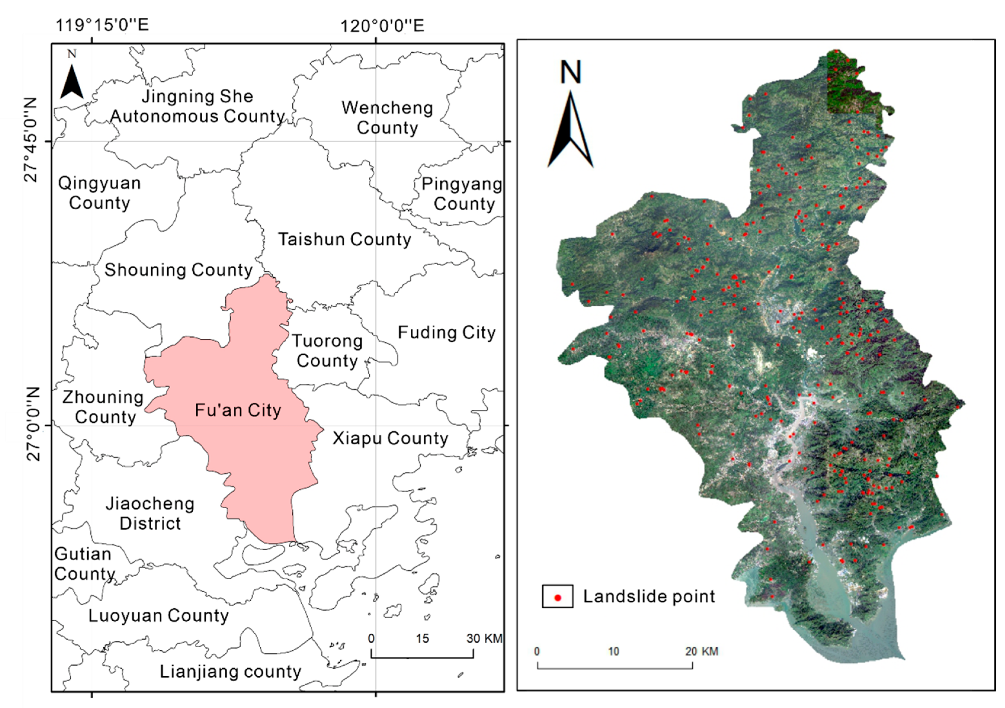
2.1. Study Area

The study area is Fu’an City, Fujian Province, China, located in the northeastern part of Fujian province. As shown in Figure 1, between 119°23′~119°52′ E and 26°41′~27°24′ N, the total area is 1880 km2. The study area is located near the ocean, the climate is warm and humid, and the climate is a subtropical marine monsoon climate. The study area contains three major mountain ranges: the southeast slope of the Jiufeng mountains, the southwest Taimu mountains, and the Donggong mountains. The mountain trend is roughly northeast-southwest, and the terrain is inclined to the south. The east and west are high, and the middle is low-lying. The study area forms a north-south valley. The stratigraphic Mesozoic in the study area has an extensive distribution range, and the Cenozoic and Sinian sub-world are only exposed in small spaces. Landforms are divided into five types: mountains, hills, valleys, plains, and beaches [32].

2.2. Data Sources

The primary data sources are: (1) Field investigation and relevant landslide data obtained by Fu’an Natural Resources Bureau; (2) From Geospatial Data Cloud (https://www.gscloud.cn/) (accessed date: 19 November 2021), 30 m resolution DEM data and Landsat 8 remote sensing images to extract elevation, slope, NDVI, plane curvature, profile curvature, river system distance, slope aspect, and other information, as shown in Figure 2; (3) A 1:200,000 geological map to obtain the lithological data of the study area, as shown in Figure 2h.

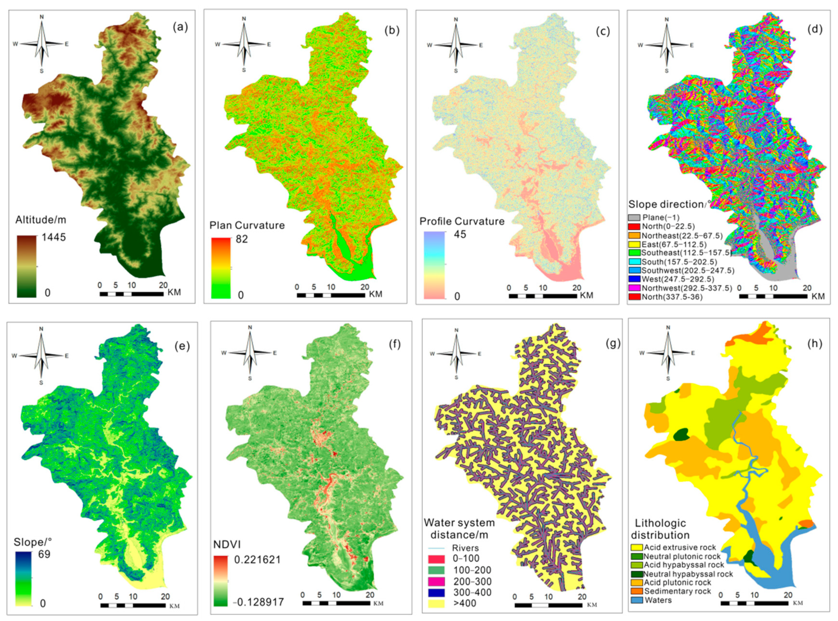
2.3. Environmental Factors
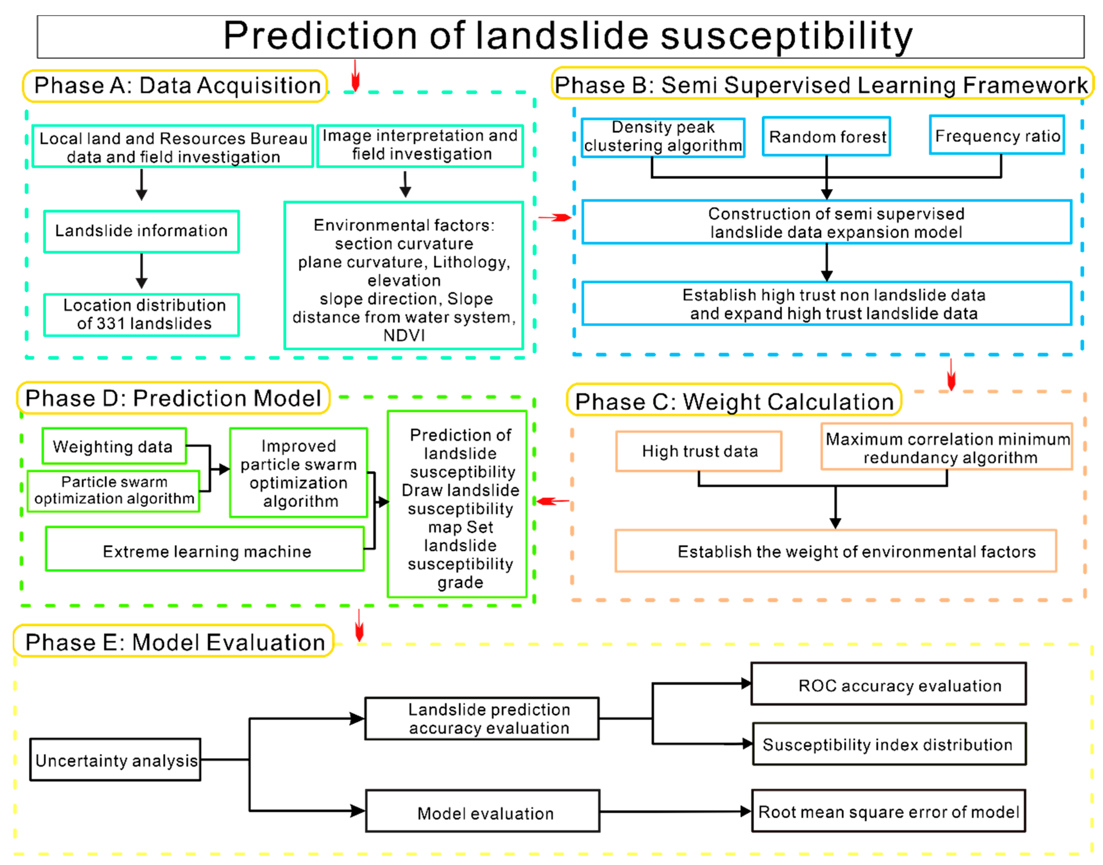
According to the geographical situation of Fu’an City, the existing landslide research, and the introduction of relevant references, most of the landslides in Fu’an City are located in relatively high terrain. Landslides are mainly distributed over the eastern and surrounding areas and more minor in the central and western regions. This paper extracts eight landslide environmental factors: elevation, slope, NDVI, plane curvature, section curvature, water system distance, slope aspect, and lithology.

3. Methods

The flow of the SS-PSO-ELM model proposed in this paper is shown in Figure 3: (1) Landslide location information and environmental factor data in the study area are obtained based on field surveys; (2) A semi-supervised learning framework is constructed based on a density peak clustering algorithm, random forest model, and frequency ratio method, and using a semi-supervised learning framework to convert landslide information and environmental factor data from field surveys into high-trust non-landslide data and landslide data; (3) High-trust data are weighted using a max-correlation min-redundancy algorithm; (4) The weighted data are substituted onto the PSO-ELM model to predict landslide susceptibility and draw a landslide susceptibility map; (5) Using ROC curve, landslide susceptibility index, and root mean square error, the prediction accuracy of the landslide is evaluated, to provide new research ideas and theoretical guidance for landslide susceptibility prediction.

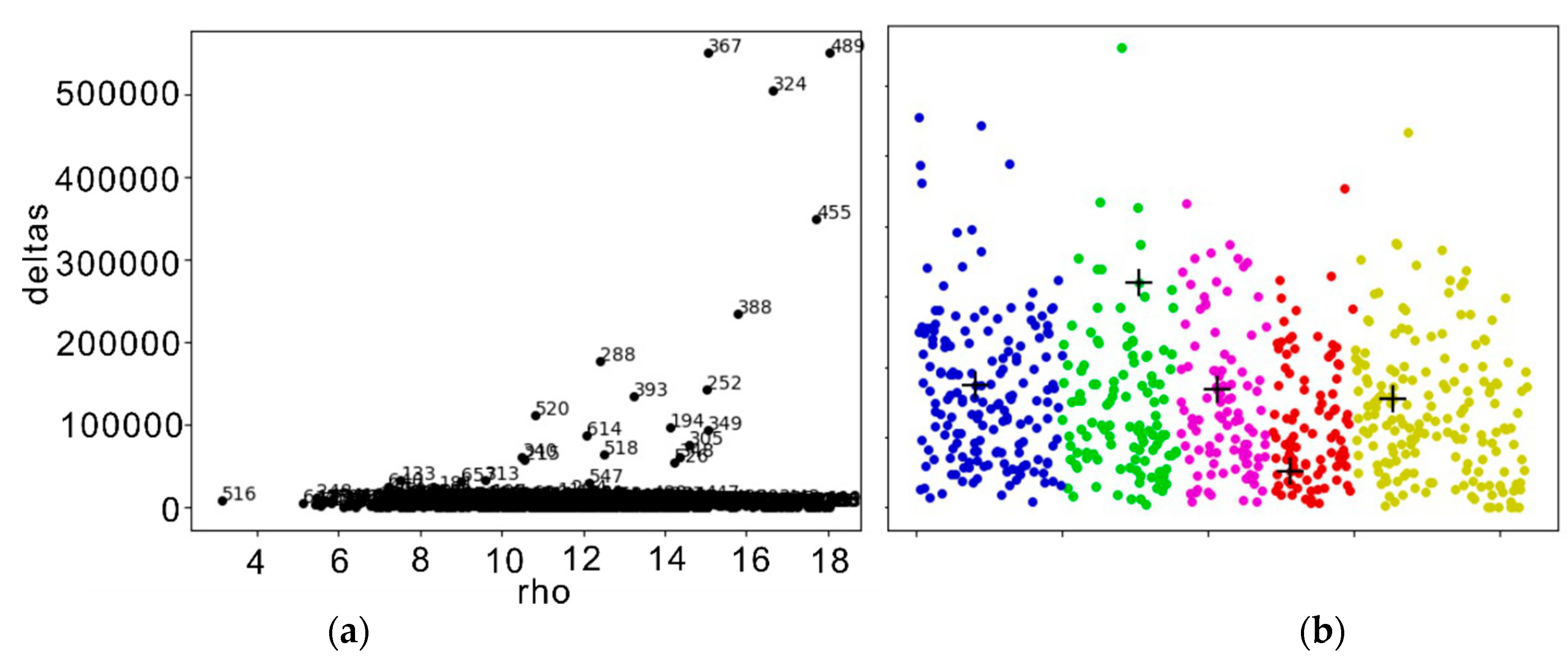
3.1. Density Peak Clustering Algorithm

The density peak clustering algorithm is a new clustering algorithm proposed by Rodriguez in 2014 [33]. The algorithm has the advantages of the mean clustering method, hierarchical clustering method, grid clustering algorithm, and density clustering algorithm, which are fast and straightforward, and insensitive to noise, and overcomes the shortcomings of the high computational complexity of the existing traditional clustering algorithms. The density peak clustering algorithm defines new clustering metrics: Minimum Density Distance and Local Density. The algorithm uses low-density areas to distinguish high-density areas and can quickly and effectively identify cluster centers in many data. This is suitable for data of any distribution type [34].
Let the local density be ρ , the minimum density distance be δ , the local density of the data point x a be ρ a , and the reach of data point x a to the nearest data point x b whose local density is more significant than itself be δ a .
The local density formula of the density peak clustering algorithm is:
ρ a = a b χ ( d a b d c )
The minimum density distance formula is:
δ a = min b : ρ b > ρ a ( d a b )
In the procedure, χ ( ) is the logical judgment function, ( ) < 0 , χ ( ) = 1 , otherwise χ ( ) = 0 , d a b is the distance between x a and x b , and d c is the cut-off distance. Take δ as the abscissa and ρ as the ordinate to get the clustering decision diagram of the density peak clustering algorithm. Select several points of the relatively large distance between local density and minimum density as cluster center points and remove noise points with relatively low local density but rather large minimum density distance. Finally, the data close to the cluster center are grouped into a cluster to complete the clustering.

3.2. Max-Correlation Min-Redundancy Algorithm

The maximum correlation minimum redundancy algorithm was first proposed by Peng [35] to extract optimal eigenvalues. The algorithm’s core is to find the feature of the most significant correlation between the dependent variable and the little correlation between the independent variables in a part set to delete and simplify the feature set and eliminate redundant variables.
The maximum correlation minimum redundancy algorithm calculates the correlation and redundancy between features based on mutual information. Let the two variables be X and Y . The mutual information formula is:
I ( X ; Y ) = P ( x , y ) log P ( X , Y ) P ( X ) P ( Y ) d X d Y
where P ( X , Y ) is the joint probability function of X and Y and P ( X ) and P ( Y ) are the probability density functions of X and Y , respectively. Mutual information can be understood as the amount of data that contains the Y variable in the X variable.
The maximum correlation is defined as:
max D ( S , c ) D = 1 s i = 1 s I ( x i ; c )
The minimum redundancy is defined as:
min R ( S ) R = 1 S 2 i = 1 s 1 j = i + 1 s I ( x i , x j )
where S is the feature set composed of factors, c is the target value, and I ( X i ; c ) is the mutual information between the factor features and the target.
The feature selection criteria of the maximum correlation minimum redundancy algorithm are:
Information subtraction:
max φ ( D , R ) φ ( D , R ) = D R
Information entropy:
max φ ( D , R ) φ ( D , R ) = D / R
According to information entropy or information subtraction, the total score of correlation and redundancy between factors is obtained. Then, factors are selected to be removed based on the score or the weight of each factor is calculated.

3.3. Extreme Learning Machine

Huang [36] proposed the extreme learning machine, which improved the traditional feedforward neural network’s slow learning speed, making it easy to fall into a local minimum, making it easy to overtrain, and causing the generalization performance to decline. Extreme Learning Machine is a machine learning based on a feedforward neural network. The innovations include: (1) The connection weights and thresholds of the input layer and the hidden layer can be set randomly; there is no need to adjust after setting, reducing the amount of calculation. (2) The weight between the hidden layer and the output layer does not need to be iteratively adjusted and is converted into a method for solving the equation system.
The calculation process of extreme learning machine can be expressed as:
f L ( x ) = i = 1 L β i g ( w i x j + b j ) , j = 1 , , N
where L is the number of hidden units, β i is the weight vector between the ith hidden layer and the output layer, g is the activation function, b is the bias vector, w i is the weight vector between the input layer and the hidden layer, and N is the number of training samples.
T = H β
Formula (8) can be transformed into Formula (9), where H is the output matrix of the hidden layer, β is the output weight, and T is the output result. Once the input weight w i and the paranoid vector b are randomly determined, the output matrix H is uniquely determined, and the output weight β can be determined.
β ^ = H T
In Formula (10), H is the Moore-Penrose generalized matrix of H .
Y = H ' β ^
Substitute the test set into Formula (10) to calculate the hidden layer output matrix H ' , and obtain the test set result.

3.4. Random Forest

Breiman first proposed random forest [37]. Random forest is based on a decision tree model. A more stable model is obtained by fusion of multiple decision trees, combining a random selection of features and integration ideas. The model randomly selects components and samples, so each tree has differences and similarities. Each tree predicts the pieces and obtains the final decision through voting [3].

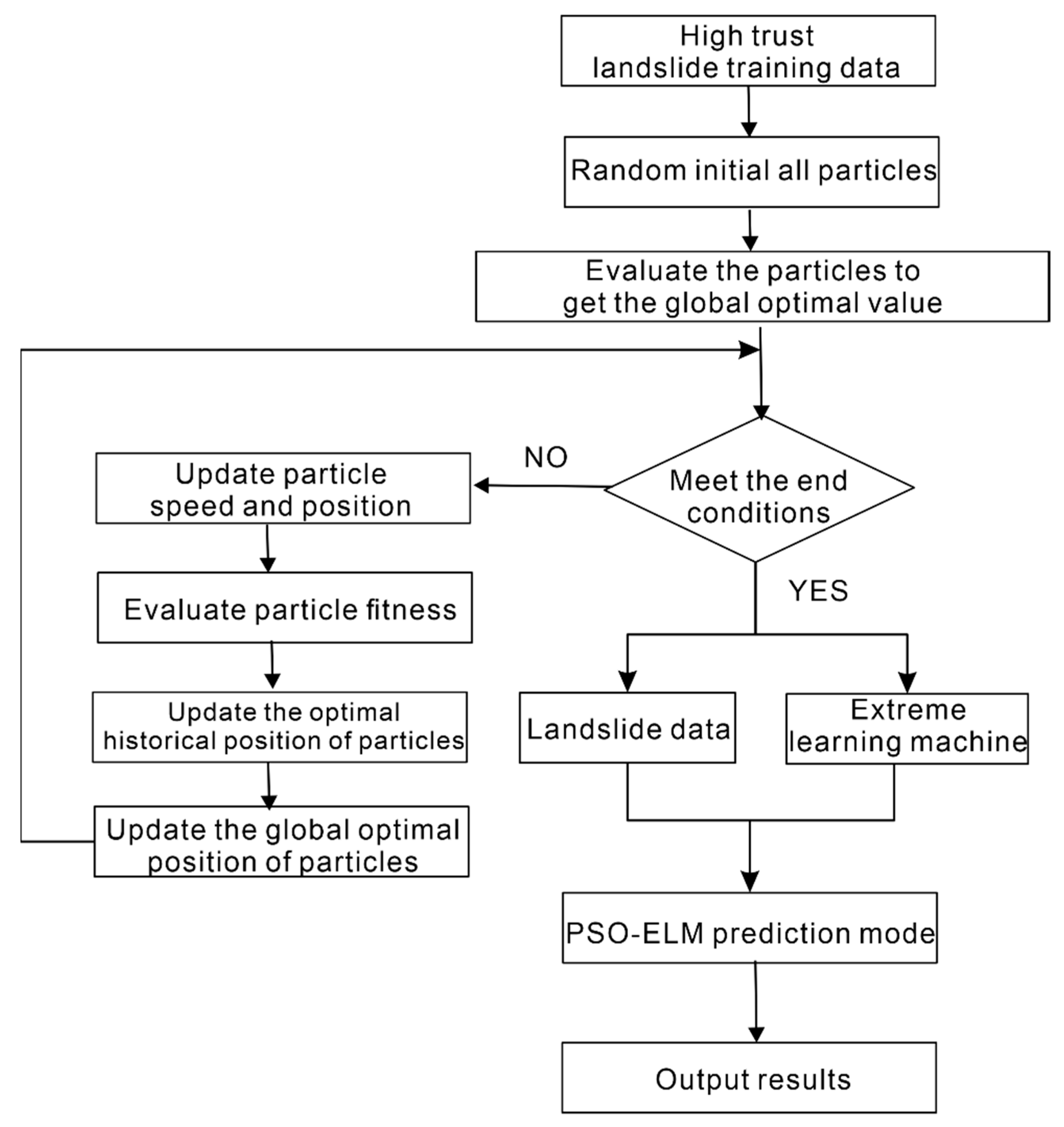
3.5. Particle Swarm Optimization Algorithm

Particle swarm optimization is an evolutionary algorithm that imitates the foraging behavior of birds, first proposed by Kennedy and Eberhart [38,39]. Particle swarm optimization has the advantages of fast convergence speed and high optimization performance. Moreover, it will not fall into a local optimum.
The core of particle swarm optimization is that in the D-dimensional particle search space, there are n particles. All particles have a fitness value determined by the optimized function. Each particle’s vector velocity determines the distance and direction they fly. The particles will follow the current optimal particle to search in the space, and finally, all converge to the vicinity of the optimal value [40].

3.6. Uncertainty Analysis Method

3.6.1. ROC Curve Precision Analysis

The ROC curve is drawn by taking the valid positive rate (sensitivity) as the ordinate and the false positive rate (1-specificity) as the abscissa. The closer the curve is to the upper left corner, the higher the accuracy, and the larger the area under the ROC curve, the better the effect. The ROC curve indicator is defined as:
Sensitivity:
S S T = T P T P + F N
Specificity:
S P F = T N T N + F P
From the sample results, the data can be divided into two categories. For example, in this paper, the positive data are the sample data of landslides, and the negative data are the non-landslide sample data. (1) TP: Positive data predict the correct number. (2) TN: Negative data predict the correct number. (3) FP: Number of positive data prediction errors. (4) FN: Number of negative data prediction errors. (5) SST: The proportion of positive samples that are correctly classified. (6) SPF: The proportion of negative samples that are correctly classified.

3.6.2. Frequency Ratio

The frequency ratio reflects the distribution of factors of the class and can well explain the intrinsic relationship between factors and classes [41]. The formula for calculating the frequency ratio is:
F R = N j / N S j / S
where N j is the number of landslide grids in a cluster, N is the number of landslide grids in all groups, S j is the number of units in the bunch, and S is the total number of grids shared by all clusters.

3.6.3. Root Mean Square Error Analysis

The root mean square error is the square root of the square ratio of the deviation from the observed value and the actual value and the number of observations n. RMSE is very sensitive to the large and small errors of measurement data, so RMSE can well reflect the accuracy of the measurement. The mathematical formula for the root mean square error is:
R M S E = 1 n i = 1 n ( y ^ i y i ) 2
where y ^ i is the actual value, y i is the predicted value, and n is the number of observations.

4. Modeling of Landslide Susceptibility Assessment in Fu’an

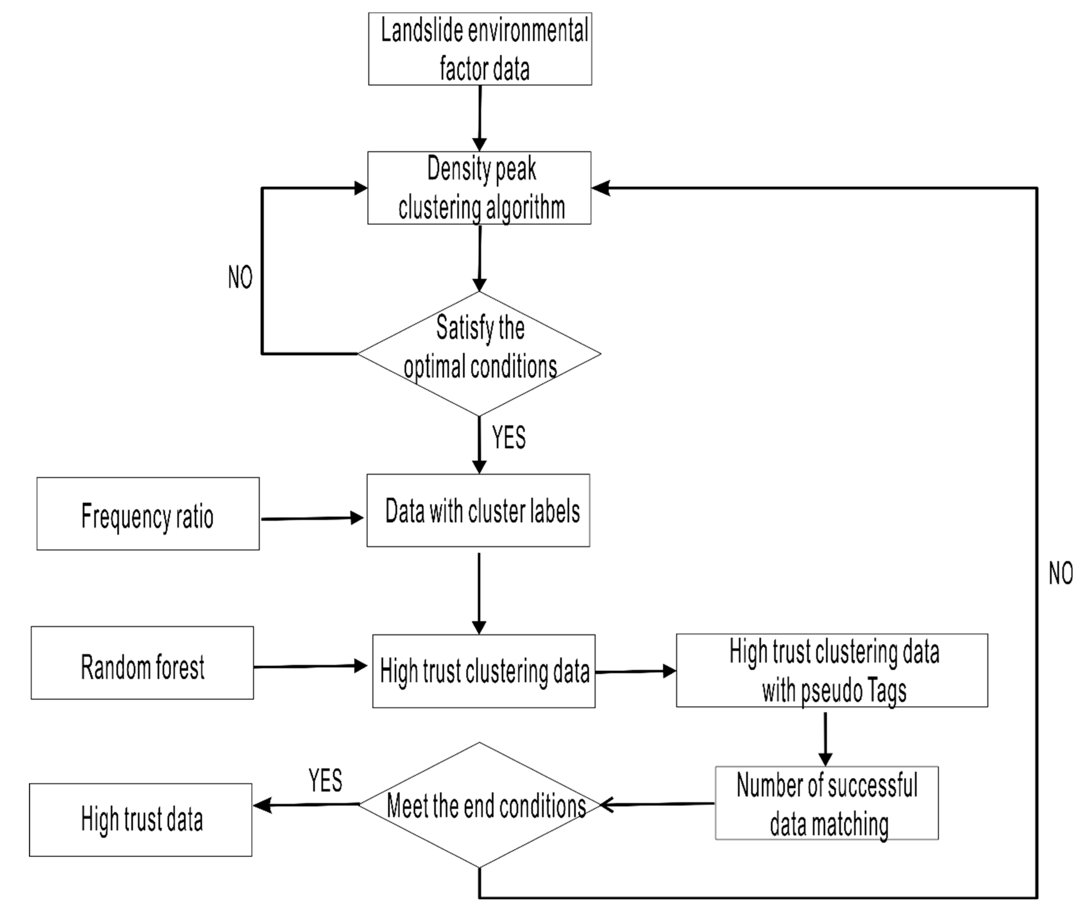
4.1. Semi-Supervised Learning Framework Construction

Before making a landslide susceptibility prediction, high-trust non-landslide points were selected and high-trust landslide points were expanded to compensate for the lack of landslide data and the uncertainty caused by the random selection of non-landslide problems.
The flowchart of the semi-supervised learning framework is shown in Figure 4: (1) The data of the study area were organized into raster data. A total of 2,191,350 grid cells were obtained in the study area, with randomly selected 622 raster cell data from which landslide data and non-landslide data are 1:1, and the 622 data are clustered by the density peak clustering algorithm, as shown in Figure 5. Figure 5a is the cluster center selection diagram, the abscissa is the density of data points, and the ordinate is the distance from the point to the nearest higher density point. The density peak clustering algorithm selects a point with a higher density and no higher density nearby as the cluster center point. Therefore, according to Figure 5a, 489, 324, 367, 455, and 388 were selected as the cluster center points. Figure 5b shows that the remaining points are divided according to the five cluster center points. All the data are divided into five categories, and the cross symbols indicate the positions of the five cluster centers. (2) The categories calculated by the clustering algorithm were analyzed according to the frequency ratio method, and category a, with the most landslide data, and category b, with the most non-landslide data, were selected. The optimal condition is that both the proportion of landslide data in a and the ratio of non-landslide data in b exceed 0.7 (according to the existing research foundation and multiple experiments, it has been proved that 0.7 is the best threshold for experimental results; less than 0.7 is not ideal, and data with a threshold over 0.7 are prone to local redundancy). Otherwise, repeat step 1. The meaning of this step is to select two types of data from the five types of data, one of which has a landslide ratio higher than 0.7 and the other type of data whose non-landslide percentage is higher than 0.7. According to the density peak clustering algorithm, the same kind of data approximates in space if the proportion of landslide or non-landslide in a data class is the majority. It can be demonstrated that landslides or non-landslides in such data may be a standard feature. (3) The high-trust clustering data is used as training data on the random forest. Predict existing high-trust clustered data (the data for the first loop is itself). Assign prediction results to pseudo labels. In this step, the cluster data obtained in the above steps are added to the training data of the random forest model, and then the data are predicted and classified. Suppose the label of the predicted class is the same as the label of the previous step. The credibility of this piece of data will increase. (4) Add frequency labels. When the pseudo-labels and clustering labels are the same, the frequency label is increased by one. When the number of program loops gradually increases, the training data of the random forest will also gradually increase, which will cause the prediction results of the random forest model to fluctuate. As the number of loops increases, the larger the value of the frequency label, the more it can be proved that when the training data increase, the data have little effect on it. It is proved that the landslides (non-landslides) in the data have more in common with the data of multiple cluster classifications, indicating that the cluster labels of the data are more credible. (5) Determine whether the value of the frequency label reaches the threshold set by the end condition (when the frequency label value of a certain piece of data reaches 10, select all data with a frequency label greater than seven as high-confidence data). If not, return to step 1. Change the raster data selection method selected in step 1. A random selection of 622 cell data from all raster cells, regardless of the proportion of landslide and non-landslide data. Moreover, the data were compared with existing high-confidence data to remove redundant data.
The final high-trust data obtained are shown in Table 1. The more matching values, the higher the reliability of the data, and the smaller the number of matching values, which proves that the data fluctuate wildly and cannot be accepted as high-trust data.
Figure 6 shows the high-trust non-landslide points distribution in the study area. It can be seen from Figure 6a that a large part of the high-trust non-landslide point data are on the water surface. Figure 6b shows that most high-trust non-landslide point data are distributed over low-altitude areas, proving that it is advisable to adopt a semi-supervised framework to select high-trust non-landslide points.

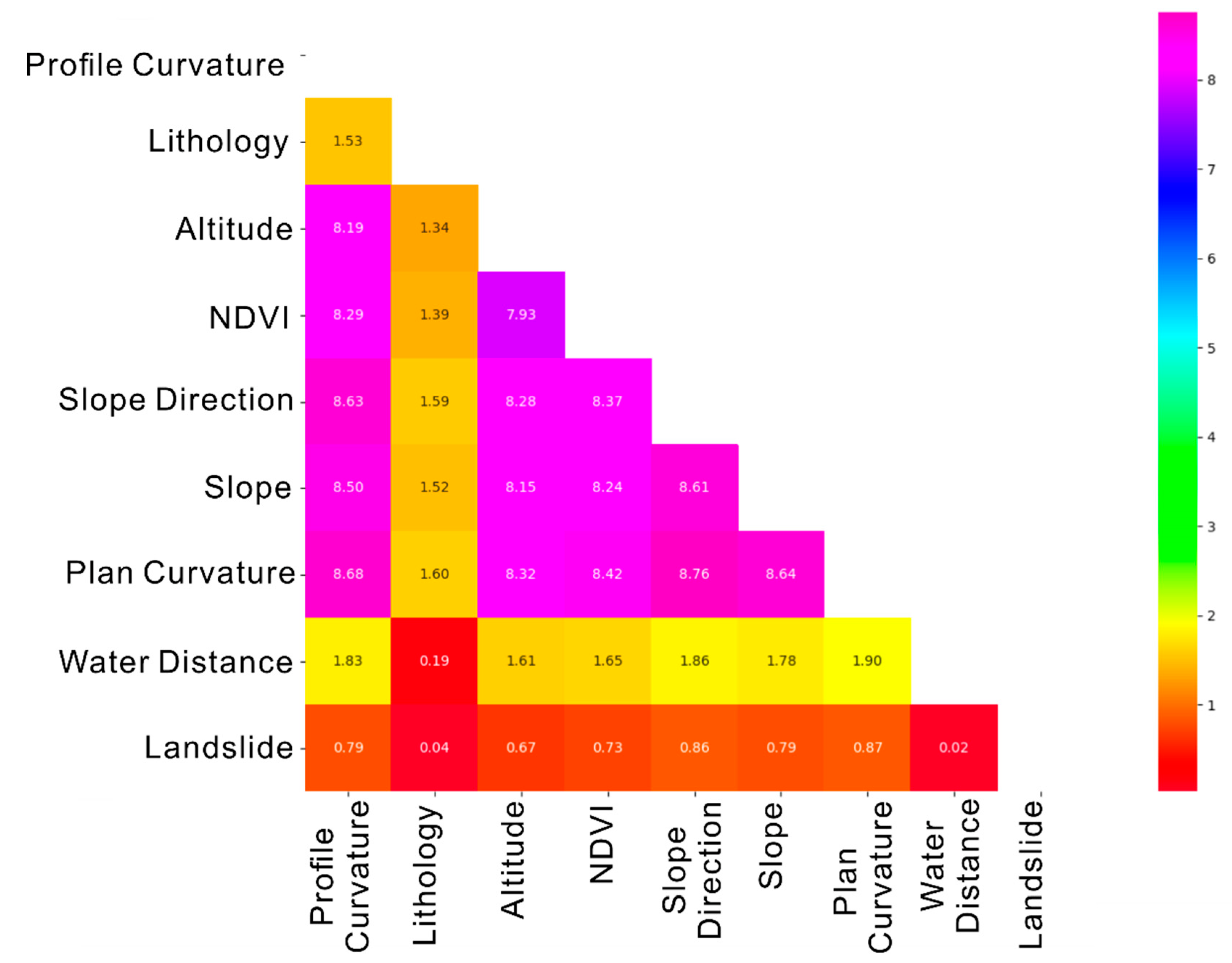
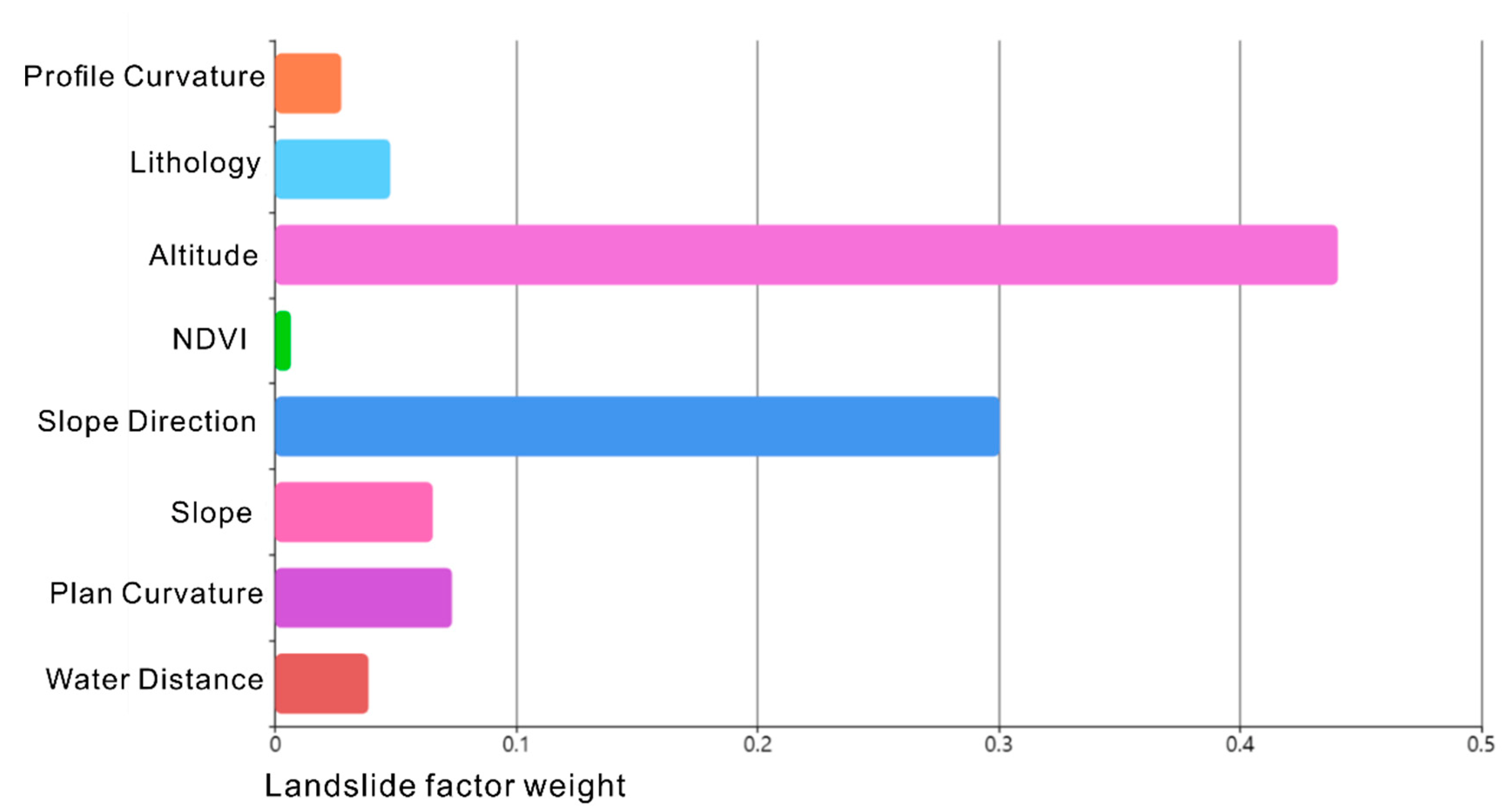
4.2. Weight Determination Analysis

Based on the high-trust data obtained above, the maximum correlation minimum redundancy algorithm is used to calculate the weight of the landslide environmental factors. The mutual information on each environmental element and the landslide is shown in Figure 7, and the weights of environmental factors are shown in Figure 8. Mutual information represents the amount of information one random variable contains in another. Therefore, the higher the mutual information, the closer the relationship between the two variables. Figure 7 shows the mutual information between various environmental factors. It can be seen from the mutual information between each environmental element and landslide in Figure 7 that the mutual information between the slope aspect and landslide is the largest, with a value of 0.86. However, in the final weights shown in Figure 8, the influence of the slope direction on the landslide is ranked second. The slope direction and landslide have high mutual information, and the slope direction and other environmental factors also have high mutual information. Therefore, when the slope direction is used as the input for landslide prediction, if the weight of the slope direction is too high, it will lead to more redundancy and more significant prediction errors. Therefore, in the final weights calculated by the maximum correlation minimum redundancy algorithm, the weight of the slope direction is less than the weight of the elevation. This proves that it is feasible to calculate the importance of the landslide factor based on the maximum correlation minimum redundancy algorithm.

4.3. PSO-ELM Prediction Model

The model flow of the extreme learning machine optimized by the particle swarm optimization algorithm is shown in Figure 9: (1) To posit the velocity of the random particle swarm; (2) To evaluate the fitness value of all particles to get the optimal global position; (3) To update the velocity and position of each particle; (4) To evaluate the optimal fitness value of each particle of the previous iteration process, compare it with its own historical optimal fitness value, and select a better one; (5) To update the optimal global position—each particle moves towards the optimal global position and its optimal historical position; (6) To predict landslide susceptibility by assigning optimal parameters to an extreme learning machine.

4.4. Landslide Susceptibility Mapping
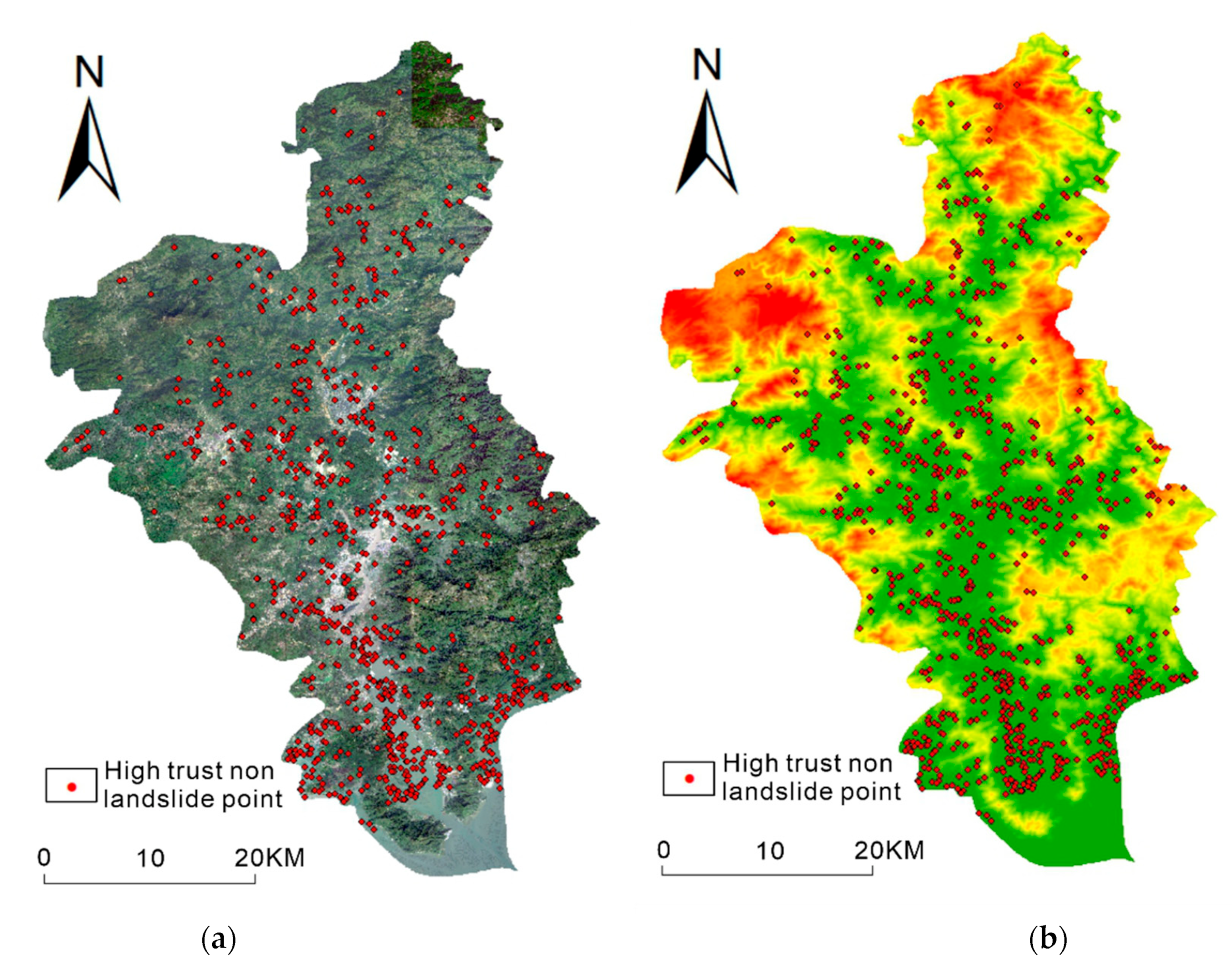
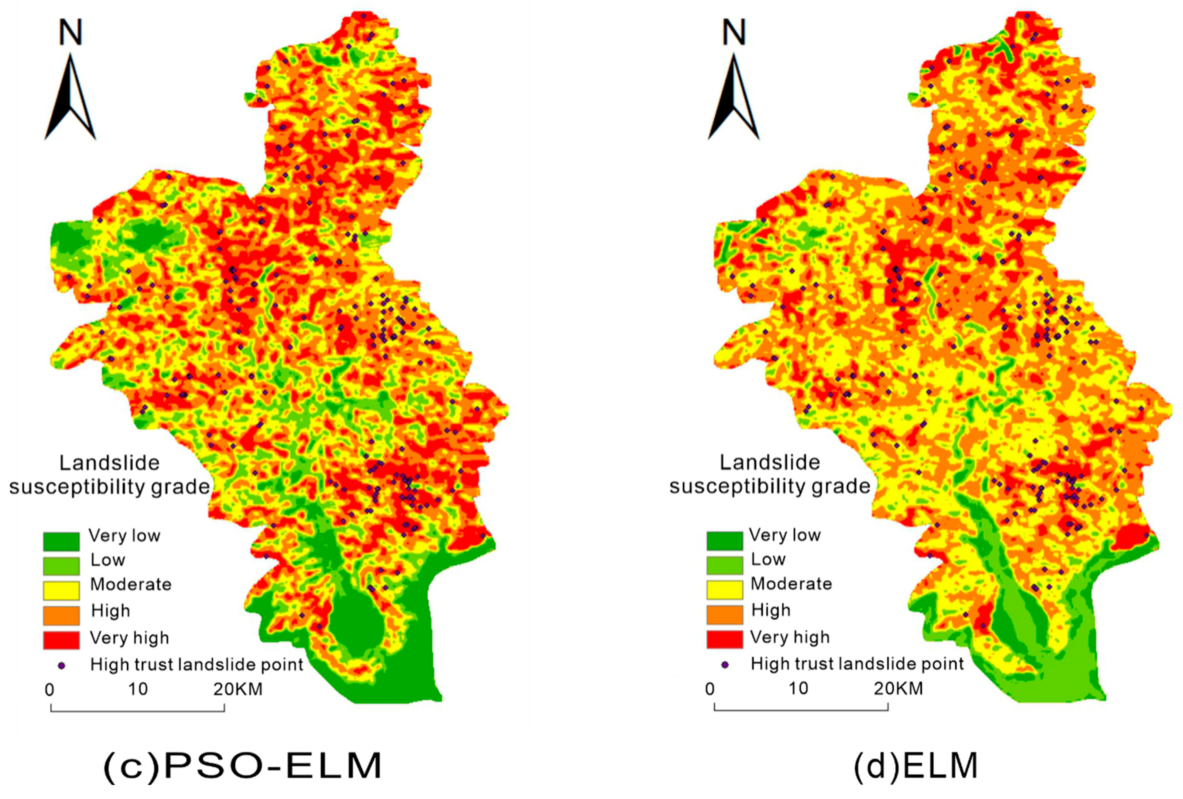
The landslide susceptibility mapping of the study area is shown in Figure 10. The natural discontinuity method divides landslide susceptibility into five zones: very low, low, medium, high, and very high. Figure 10 indicates that:
(1)
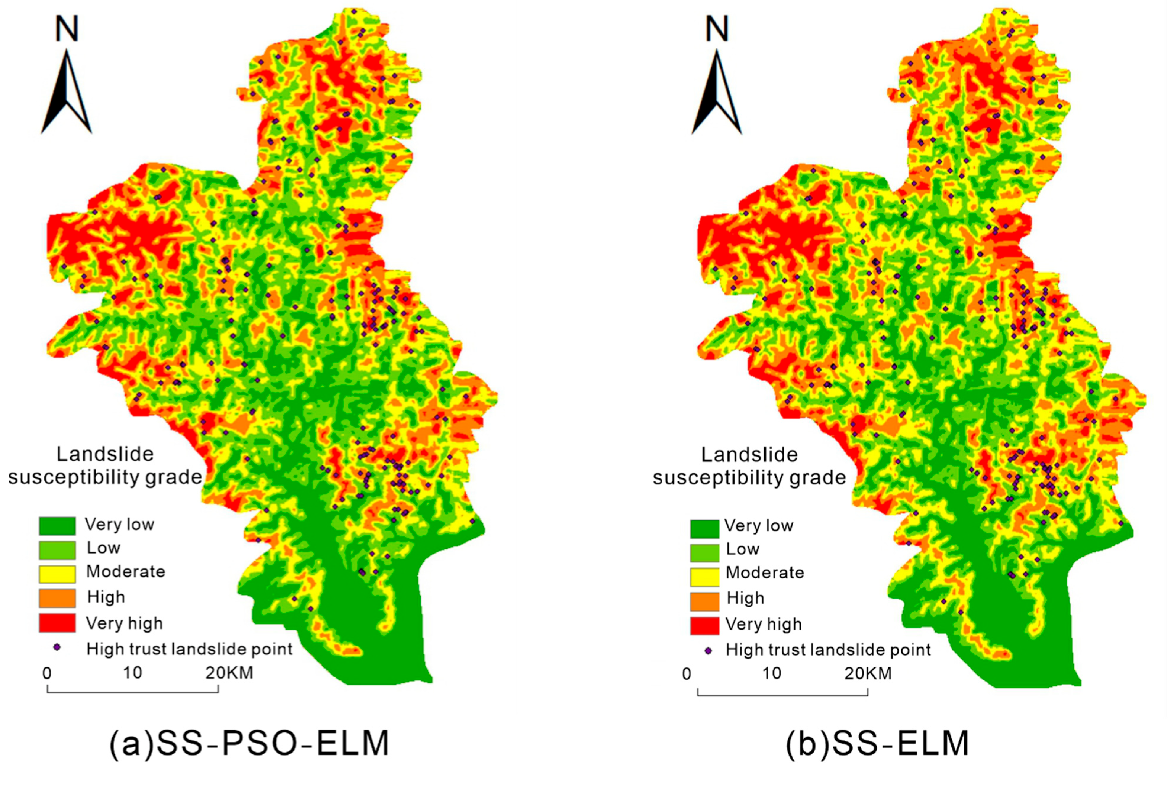
The landslide points in the figure are landslide high-trust points expanded by the semi-supervised learning framework. Because the original landslide point may be accidental, it may be difficult for subsequent landslides to occur in this area over time. Therefore, this paper uses the expanded landslide high-confidence points to test the landslide susceptibility mapping.
(2)
The results of the four models, SS-PSO-ELM, SS-ELM, PSO-ELM, and ELM, are shown in the figure. The high-trust landslide points all fall in the high-risk and very high-risk areas, proving that the four models can effectively predict landslides. However, in the PSO-ELM model and the ELM model, the high-risk and very high-risk areas account for a large proportion of the entire study area, which is inconsistent with reality. The SS-PSO-ELM model and the SS-ELM model are more realistic.
(3)
In the northwest corner of the study area, the SS-PSO-ELM model and the SS-ELM model predicted a very high-risk area. The prediction results in the PSO-ELM and ELM models are low-risk and very low-risk areas. After data inspection and analysis, the reason is that the non-landslide points of the model without the semi-supervised learning framework are randomly selected in the study area. However, randomly selected points within the study area do not guarantee that they are credible non-landslide points. As shown in this case, the area that was initially a high risk of the landslide was used as a sample to enter the training data into non-landslide points, resulting in a large discrepancy between the results and the actual results.

5. Modeling Uncertainty Analysis

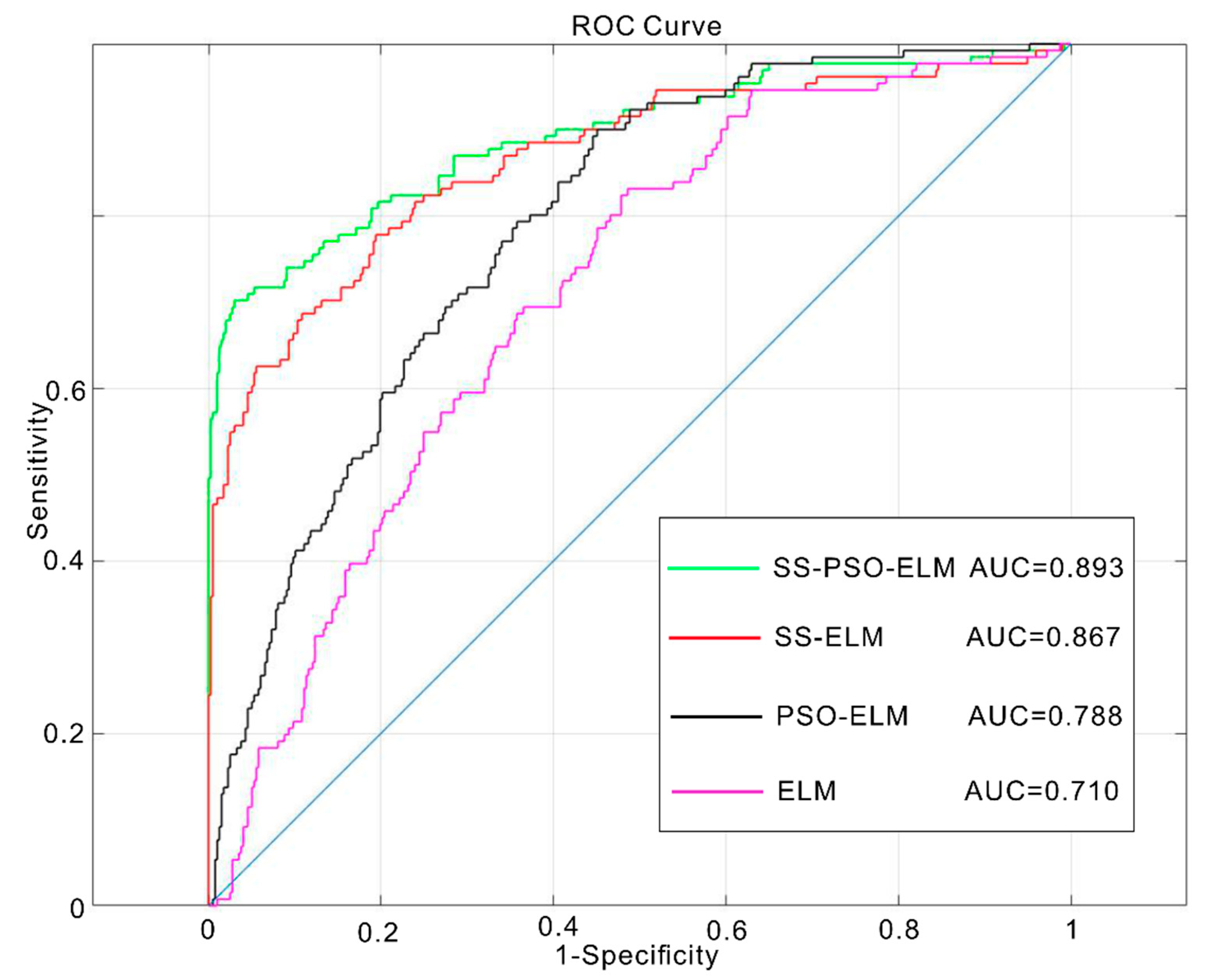
5.1. ROC Accuracy Evaluation

As shown in Figure 11, the model’s prediction accuracy is evaluated by the AUC area under the ROC curve. The AUCs of SS-PSO-ELM, SS-ELM, PSO-ELM, and ELM was 0.893, 0.867, 0.788, and 0.710, respectively. From the image, SS-PSO-ELM and SS-ELM have better prediction performance of landslide susceptibility. However, the curve of the SS-ELM model rises slowly in the later stage, and the prediction performance fluctuates wildly. Furthermore, this proves that the extreme learning machine model optimized by particle swarm optimization algorithm has higher accuracy and stability in landslide susceptibility prediction. The AUC accuracy of the SS-PSO-ELM model is 0.105 more increased than that of the PSO-ELM model without the semi-supervised learning framework. This shows that using a semi-supervised learning framework to screen non-landslide high-trust points can significantly improve the performance of landslide susceptibility prediction.

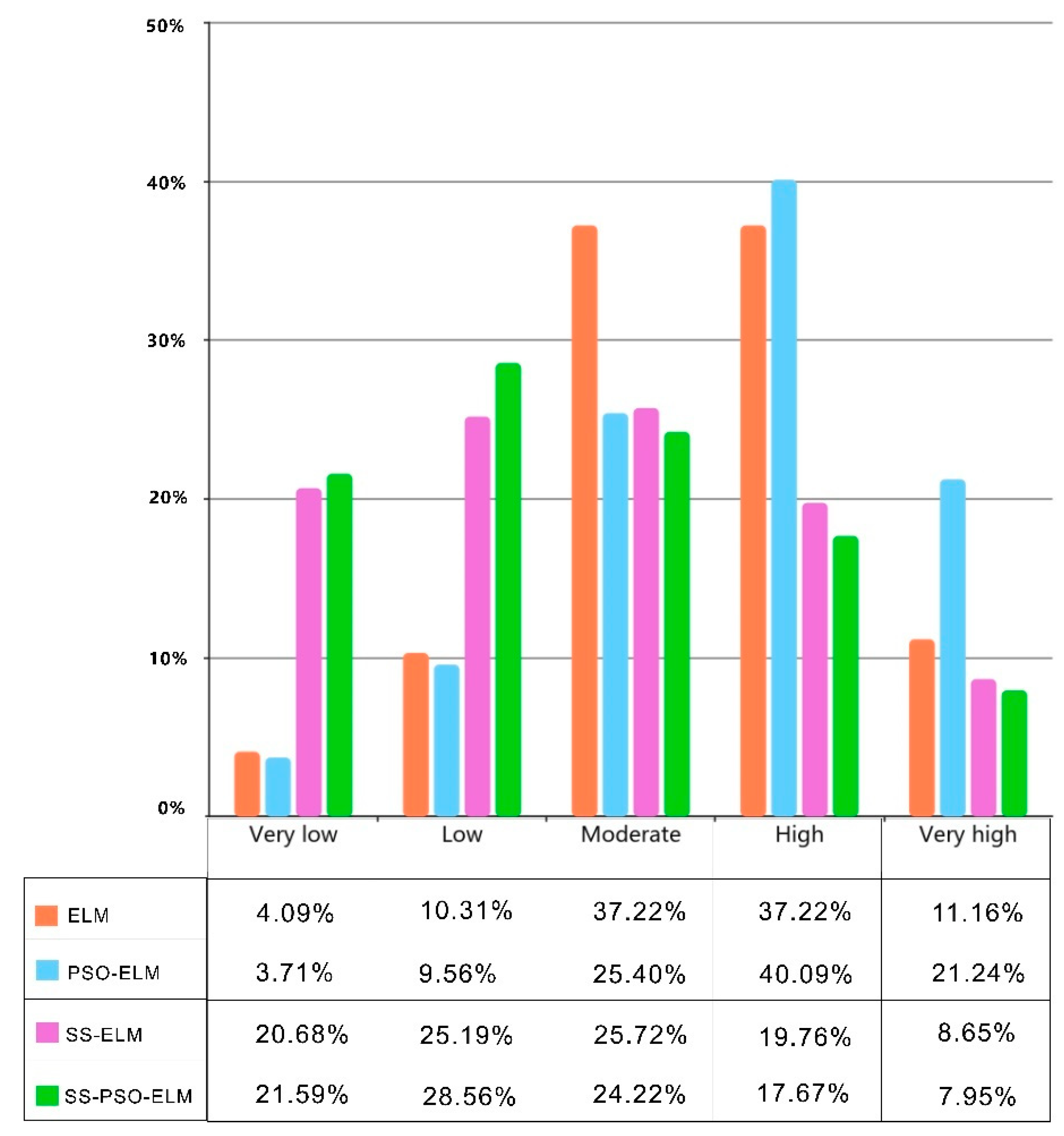
5.2. Susceptibility Index Distribution

The distribution of the susceptibility index can visually observe the number of individuals in the specific susceptibility index interval in the study area. In practice, the range of landslide sites is much smaller than that of non-landslide sites. Therefore, we will focus on the very high-risk and very low-risk areas’ scale when judging the model’s performance in landslide susceptibility prediction. The larger the scale of the two areas, the better the model’s ability to identify landslides. Therefore, the distribution of the susceptibility index can intuitively see the proportion of each risk area of the model and can more intuitively reflect the predictive performance of the model.
Figure 12 shows the susceptibility index distribution, showing the amount included in each landslide probability interval. The mean and standard deviation is shown in Figure 12 can better reflect the prediction level of the four models and the dispersion degree of the predicted landslide data. Figure 13 demonstrates the proportion of each landslide-prone zone in the study area. Both figures can show the stability of the model for landslide prediction and judge whether the model prediction is in line with the actual situation.
(1)
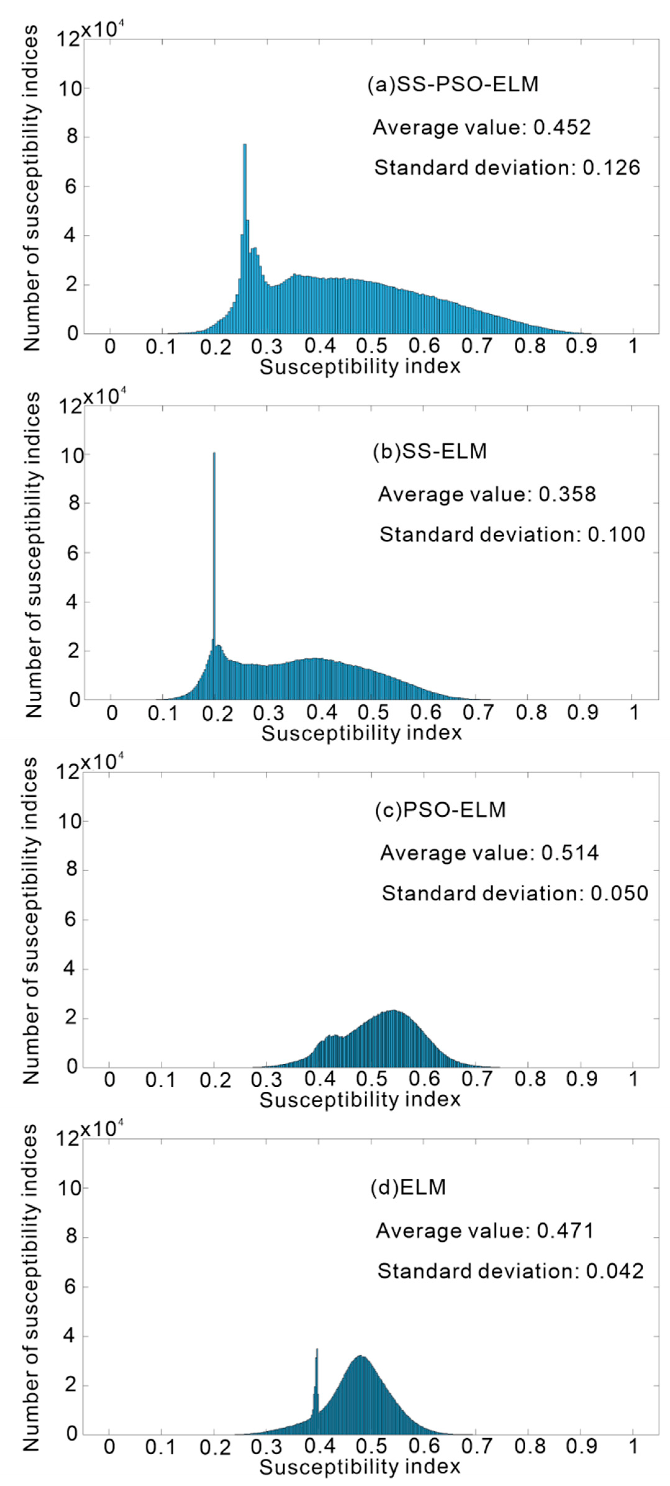
The landslide risk areas of the SS-PSO-ELM model and the SS-ELM model are concentrated in low-risk and very low-risk areas and less in high-risk and very high-risk areas. The overall trend of landslide susceptibility is that the area from low risk to high risk gradually decreases, which is more in line with reality.
(2)
The mean value of landslide occurrence probability of SS-PSO-ELM and SS-ELM models is smaller than that of the PSO-ELM model and ELM model. It is proved that the semi-supervised learning framework’s prediction of landslide susceptibility is in line with reality, and the extremely low-susceptibility and low-susceptibility areas of landslides are the mainstream in the study area.
(3)
In Figure 12, the standard deviations of the four models are compared from large to small, namely SS-PSO-ELM, SS-ELM, PSO-ELM, and ELM. The SS-PSO-ELM standard deviation is the largest, proving that the SS-PSO-ELM model can distinguish and identify landslides and better reflect the differences in landslide susceptibility to the study area. However, since the PSO-ELM and ELM models do not use high-trust non-landslide points as training data, the probability of landslides in most places is concentrated between 0.4 and 0.6, and there is no good ability to discriminate landslides. Furthermore, most of the predicted areas are in the high-risk prone regions to landslides, which is inconsistent with the actual situation.

5.3. Model Evaluation

The evaluation indexes of each model are shown in Table 2. The RMSE of the particle swarm optimized SS-PSO-ELM model is smaller than that of the PSO-ELM model. Furthermore, the small model volatility indicates that the extreme learning machine model optimized by the particle swarm optimization algorithm has significantly improved the landslide susceptibility prediction performance. The AUC values of the SS-PSO-ELM model and the SS-ELM model are higher than those of the PSO-ELM model and the ELM model, proving that the semi-supervised learning framework can significantly improve the performance of the model. Figure 12 and Figure 13 and Table 2 indicate that SS-PSO-ELM has a higher performance in predicting landslide susceptibility, which is more in line with reality.

6. Conclusions

This paper takes Fu’an City, Fujian Province, as the research object and selects eight environmental factors: elevation, slope, NDVI, plane curvature, section curvature, water system distance, slope aspect, and lithology. A model evaluating landslide susceptibility is established with semi-supervised learning as the framework and the extreme learning machine of particle swarm optimization as the driving model. A comparative analysis was conducted with SS-ELM, PSO-ELM, and ELM as contrast models.
The SS-PSO-ELM model has the highest AUC accuracy, indicating that the model has the best performance in landslide susceptibility prediction. The mean value of SS-PSO-ELM is small, which is in line with the actual situation because the landslide area in the study area is much smaller than the non-landslide area. The standard deviation of SS-PSO-ELM is the largest, which proves that the landslide probability values of landslide sites are higher, the landslide probability values of non-landslide sites are lower, and they have better landslide identification ability. In addition, the RMSE of the SS-PSO-ELM model is the smallest, proving that the model is less volatile in landslide susceptibility prediction.
The high-trust landslide points and high-trust non-landslide points selected according to the semi-supervised learning framework can effectively improve the accuracy of landslide susceptibility prediction by the data-driven model. High-trust landslide points can delete occasional landslide points, avoiding the problem of many high-risk and very high-risk areas when data-driven models predict landslide susceptibility, which is more in line with this reality.
Because the purpose of the clustering algorithm is to cluster similar data together, it may lead to overfitting of the high-trust non-landslide data, and the selected high-trust non-landslide data may belong to an approximate area or a geographically similar area. In the next step, the research area can be divided into several areas to ensure that the number of grid cells in each area can meet the highest performance of the clustering algorithm and the diversity of data. The landslide sensitivity of the prediction accuracy can be further improved, and the drawing is more reasonable.

Author Contributions

Conceptualization, Yizhun Zhang and Qisheng Yan; Methodology, Yizhun Zhang; Software, Yizhun Zhang; Validation, Yizhun Zhang and Qisheng Yan; Formal Analysis, Yizhun Zhang; Investigation, Yizhun Zhang; Resources, Yizhun Zhang; Data Curation, Yizhun Zhang; Writing—Original Draft Preparation, Yizhun Zhang; Writing—Review and Editing, Qisheng Yan; Visualization, Yizhun Zhang; Supervision, Qisheng Yan; Project Administration, Qisheng Yan; Funding Acquisition, Qisheng Yan. All authors have read and agreed to the published version of the manuscript.

Funding

This research was funded by [National Natural Science Foundation of China] grant number [No: 71961001].

Institutional Review Board Statement

Not applicable.

Informed Consent Statement

Not applicable.

Data Availability Statement

Not applicable.

Acknowledgments

The authors would like to thank the anonymous reviewers for their helpful and valuable comments and suggestions.

Conflicts of Interest

The authors declare that they have no known competing financial interests or personal relationships that could have appeared to influence the work reported in this paper.

References

  1. Guzzetti, F.; Carrara, A.; Cardinali, M.; Paola, R. Landslide hazard evaluation: A review of currenttechniques and their application in a multi-scale study, Central Italy. Geomorphology 1999, 31, 181–216. [Google Scholar] [CrossRef]
  2. Nadim, F.; Kjekstad, O.; Peduzzi, P.; Herold, C.; Jaedicke, C. Global landslide and avalanche hotspots. Landslides 2006, 3, 159–173. [Google Scholar] [CrossRef]
  3. Assilzadeh, H.; Levy, J.K.; Wang, X. Landslide catastrophes and disaster risk reduction:a GISframework for landslide prevention and management. Remote Sens. 2010, 2, 2259–2273. [Google Scholar] [CrossRef] [Green Version]
  4. Guzzetti, F.; Reichenbach, P.; Ardizzone, F.; Cardinali, M.; Galli, M. Estimating the quality of landslide susceptibility models. Geomorphology 2006, 81, 166–184. [Google Scholar] [CrossRef]
  5. Montgomery, D.R.; Dietrich, W.E. A physically based model for the topographic control onshallow landsliding. Water Resour. Res. 1994, 30, 1153–1171. [Google Scholar] [CrossRef]
  6. Guzzetti, F.; Mondini, A.C.; Cardinali, M.; Fiorucci, F.; Santangelo, M.; Chang, K.T. Landslide inventory maps: New tools for an old problem. Earth-Sci. Rev. 2012, 112, 42–66. [Google Scholar] [CrossRef] [Green Version]
  7. Aleotti, P.; Chowdhury, R. Landslide hazard assessment: Summary review and newperspectives. Bull. Eng. Geol. Environ. 1999, 58, 21–44. [Google Scholar] [CrossRef]
  8. Ruff, M.; Czurda, K. Landslide susceptibility analysis with a heuristic approach in theEastern Alps (Vorarlberg, Austria). Geomorphology 2008, 94, 314–324. [Google Scholar] [CrossRef]
  9. Lin, S.Y.; Lin, C.W.; Gasselt, S.V. Processing Framework for Landslide Detection Based on Synthetic Aperture Radar (SAR) Intensity-Image Analysis. Remote Sens. 2021, 13, 644. [Google Scholar] [CrossRef]
  10. Reichenbach, P.; Rossi, M.; Malamud, B.; Mihir, M.; Guzzetti, F. A review of statistically-based landslide susceptibility models. Earth-Sci. Rev. 2018, 180, 60–91. [Google Scholar] [CrossRef]
  11. Hai-Min, L.; Jack, S.; Arul, A. Assessment of Geohazards and Preventative Countermeasures Using AHP Incorporated with GIS in Lanzhou, China. Sustainability 2018, 10, 304. [Google Scholar]
  12. Khan, H.; Shafique, M.; Khan, M.A.; Bacha, M.A.; Shah, S.U.; Calligaris, C. Landslide susceptibility assessment using Frequency Ratio, a case study of northern Pakistan. Egypt. J. Remote Sens. Space Sci. 2018, 22, 11–24. [Google Scholar] [CrossRef]
  13. Bui, D.T.; Pradhan, B.; Lofman, O.; Revhaug, I.; Dick, O. BLandslide susceptibility mapping at Hoa Binh province (Vietnam) using an adaptive neuro-fuzzy inference system and GIS. Comput. Geosci. 2011, 45, 199–211. [Google Scholar]
  14. Ghorbanzadeh, O.; Shahabi, H.; Crivellari, A.; Homayouni, S.; Blaschke, T.; Ghamisi, P. Landslide detection using deep learning and object-based image analysis. Landslides 2022, 19, 929–939. [Google Scholar] [CrossRef]
  15. Ghorbanzadeh, O.; Blaschke, T.; Gholamnia, K.; Meena, S.R.; Tiede, D.; Aryal, J. Evaluation of Different Machine Learning Methods and Deep-Learning Convolutional Neural Networks for Landslide Detection. Remote Sens. 2019, 11, 196. [Google Scholar] [CrossRef] [Green Version]
  16. Ghorbanzadeh, O.; Xu, Y.; Ghamis, P.; Kopp, M.; Kreil, D. Landslide4Sense: Reference Benchmark Data and Deep Learning Models for Landslide Detection. arXiv 2022, arXiv:2206.00515. [Google Scholar]
  17. Alb, A.; Frb, C.; Qbp, D.; Gigović, L.; Drobnjak, S.; Aina, Y.A.; Panahi, M.; Yekeen, S.T.; Lee, S. Spatial prediction of landslide susceptibility in western Serbia using hybrid support vector regression (SVR) with with GWO, BAT and COA algorithms. Geosci. Front. 2020, 12, 101104. [Google Scholar]
  18. Depina, I.; Oguz, E.A.; Thakur, V. Novel Bayesian framework for calibration of spatially distributed physical-based landslide prediction models. Comput. Geotech. 2020, 125, 103660. [Google Scholar] [CrossRef]
  19. Guo, Z.; Chen, L.; Gui, L.; Du, J.; Yin, K.; Do, H.M. Landslide displacement prediction based on variational mode decomposition and WA-GWO-BP model. Landslides 2019, 17, 567–583, (In Chinese with English abstract). [Google Scholar] [CrossRef]
  20. Zhang, Y.G.; Tang, J.; Liao, R.P.; Zhang, M.F.; Zhang, Y.; Wang, X.M.; Su, Z.Y. Application of an enhanced BP neural network model with water cycle algorithm on landslide prediction. Stoch. Environ. Res. Risk Assess. 2021, 35, 1273–1291. [Google Scholar] [CrossRef]
  21. Benbouras, M.A. Hybrid meta-heuristic machine learning methods applied to landslide susceptibility mapping in the Sahel-Algiers. Int. J. Sediment Res. 2022, 37, 601–618. [Google Scholar] [CrossRef]
  22. Huang, F.M.; Pan, L.H.; Yao, C.; Zhou, C.; Huang, J.; Guo, Z. Prediction Model of Landslide Susceptibility Based on Semi-Supervised Machine Learning. J. Zhejiang Univ. (Eng. Ed.) 2021, 55, 1705–1713, (In Chinese with English abstract). [Google Scholar]
  23. Huang, F.M.; Wang, Y.; Dong, Z.L.; Wu, L.Z.; Guo, Z.Z.; Zhang, T.L. Sensitivity Evaluation of Regional Landslide Based on Grey Relational Grade Model. Earth Sci. 2019, 44, 664–676, (In Chinese with English abstract). [Google Scholar]
  24. Ito, R.; Nakae, K.; Hata, J.; Okano, H.; Ishii, S. Semi-supervised deep learning of brain tissue segmentation. Neural Netw. 2019, 116, 25–34. [Google Scholar] [CrossRef]
  25. Huang, G.; Song, S.; Gupta, J.N.; Wu, C. Semi-supervised and unsupervised extreme learning machines. IEEE Trans. Cybern. 2014, 44, 2405–2417. [Google Scholar] [CrossRef]
  26. Jin, G.; Liu, C.; Chen, X. Adversarial network integrating dual attention and sparse representation for semi-supervised semantic segmentation. Inf. Processing Manag. 2021, 58, 102680. [Google Scholar] [CrossRef]
  27. Jian, C.; Yang, K.; Ao, Y. Industrial fault diagnosis based on active learning and semi-supervised learning using small training set. Eng. Appl. Artif. Intell. 2021, 104, 104365. [Google Scholar] [CrossRef]
  28. Xu, L.; Cui, L.; Weise, T.; Li, X.; Wu, Z.; Nie, F.; Chen, E.; Tang, Y. Semi-Supervised Multi-Layer Convolution Kernel Learning in Credit Evaluation. Pattern Recognit. 2021, 120, 108125. [Google Scholar] [CrossRef]
  29. Yao, J.; Qin, S.; Qiao, S.; Che, W.; Chen, Y.; Su, G.; Miao, Q. Assessment of Landslide Susceptibility Combining Deep Learning with Semi-Supervised Learning in Jiaohe County, Jilin Province, China. Appl. Sci. 2020, 10, 5640. [Google Scholar] [CrossRef]
  30. Hu, H.; Wang, C.; Liang, Z.; Gao, R.; Li, B. Exploring Complementary Models Consisting of Machine Learning Algorithms for Landslide Susceptibility Mapping. ISPRS Int. J. Geo-Inf. 2021, 10, 639. [Google Scholar] [CrossRef]
  31. Shahabi, H.; Rahimzad, M.; Tavakkoli Piralilou, S.; Ghorbanzadeh, O.; Homayouni, S.; Blaschke, T.; Lim, S.; Ghamisi, P. Unsupervised Deep Learning for Landslide Detection from Multispectral Sentinel-2 Imagery. Remote Sens. 2021, 13, 4698. [Google Scholar] [CrossRef]
  32. Liang, L.H. Analysis of Influencing Factors of Geological Hazards in Fu’an City. Fujian Geol. 2012, 31, 185–190, (In Chinese with English abstract). [Google Scholar]
  33. Rodriguez, A.; Laio, A. Clustering by fast search and find of density peaks. Science 2014, 344, 1492. [Google Scholar] [CrossRef] [Green Version]
  34. Qian, L.X.; Wang, H.R.; Dang, S.Z.; Hong, M.; Zhao, Z.Y.; Deng, C.Y. A coupling Model of Water Resources Shortage Risk Assessment and its Application. Syst. Eng. 2021, 41m, 1319–1327, (In Chinese with English abstract). [Google Scholar]
  35. Peng, H.; Long, F.; Ding, C. Feature selection based on mutual information criteria of max-dependency, max-relevance, and min-redundancy. IEEE Trans. Pattern Anal. Mach. Intell. 2005, 27, 1226–1238. [Google Scholar] [CrossRef]
  36. Huang, G.B.; Zhu, Q.Y.; Siew, C.K. Extreme learning machine: Theory and applications. Neurocomputing 2006, 70, 489–501. [Google Scholar] [CrossRef]
  37. Breiman, L. Random forests. Mach. Learn. 2001, 45, 5–32. [Google Scholar] [CrossRef] [Green Version]
  38. Kennedy, J.; Eberhart, R.C. Particle Swarm Optimization. In Proceedings of the International Conference on Neural Networks (ICNN’95), Perth, Australia, 27 November–1 December 1995; Volume 4, pp. 1942–1948. [Google Scholar]
  39. Eberhart, R.C.; Kennedy, J. A new optimizer using particle swarm theory. In Proceedings of the MHS95 Sixth International Symposium on Micro Machine and Human Science, Nagoya, Japan, 4–6 October 1995; pp. 39–43. [Google Scholar]
  40. Zhang, S.; Qian, X.M.; Lou, P.H.; Wu, X.; Sun, C. Path Planning Optimization of Large-Scale Agv System Based on Improved Particle Swarm Optimization Algorithm. Comput.-Integr. Manuf. 2020, 26, 2484–2496, (In Chinese with English abstract). [Google Scholar]
  41. Li, W.B.; Fan, X.M.; Huang, F.M.; Wu, X.L.; Yin, K.; Chang, Z. Uncertainty of Landslide Susceptibility Modeling Based on Different Environmental Factors Linkage and Prediction Models. Earth Sci. 2021, 46, 3777–3795, (In Chinese with English abstract). [Google Scholar]
Figure 1. Geographical location and landslide location map of Fu’an.
Ijgi 11 00398 g001
Figure 2. Environmental factors of landslides in Fu’an. (a) Elevation map. (b) Plane curvature map. (c) Profile curvature map. (d) Slope direction map. (e) Slope map. (f) NDVI map. (g) Water system distance map. (h) Lithology map.
Ijgi 11 00398 g002
Figure 3. Landslide susceptibility prediction modeling flowchart.
Ijgi 11 00398 g003
Figure 4. Flowchart of the semi-supervised learning framework.
Ijgi 11 00398 g004
Figure 5. Flowchart of the semi-supervised learning framework. (a) Cluster center distribution map. (b) Cluster distribution map.
Ijgi 11 00398 g005
Figure 6. High-trust non-landslide location map. (a) High-trust non-landslide satellite imagery. (b) High-trust non-landslide elevation map.
Ijgi 11 00398 g006
Figure 7. Environmental factor mutual information.
Ijgi 11 00398 g007
Figure 8. Environmental factor weight.
Ijgi 11 00398 g008
Figure 9. PSO-ELM flowchart.
Ijgi 11 00398 g009
Figure 10. Landslide susceptibility map.
Ijgi 11 00398 g010aIjgi 11 00398 g010b
Figure 11. ROC accuracy plot.
Ijgi 11 00398 g011
Figure 12. Distribution map of landslide susceptibility index.
Ijgi 11 00398 g012
Figure 13. Model classification ratio chart.
Ijgi 11 00398 g013
Table 1. Highly trusted data (excerpt).
Grid Cell NumberElevation (m)Slope Direction (°)Slope (°)Distance from Water System (m)Cluster LabelsMatch Count
1,994,4700−1.000.000No landslide10
392,36493343.9825.87100No landslide10
1,160,37530282.524.27200No landslide6
1,161,6943767.2820.70100No landslide5
153,813478109.1311.87500Landslide10
888,368429135.6644.76300Landslide10
1,784,541271203.0828.26100Landslide5
Table 2. Model evaluation metrics.
ModelMeanStandard DeviationAUCRMSE
SS-PSO-ELM0.4520.1260.8930.370
SS-ELM0.3580.1000.8670.438
PSO-ELM0.5140.0500.7880.417
ELM0.4710.0420.7100.442
Publisher’s Note: MDPI stays neutral with regard to jurisdictional claims in published maps and institutional affiliations.

