Abstract
Since landforms composing land surface vary in their properties and appearance, their shaded reliefs also present different visual impression of the terrain. In this work, we adapt a U-Net so that it can recognize a selection of landforms and can segment terrain. We test the efficiency of 10 separate models and apply an ensemble approach, where all the models are combined to potentially outperform single models. Our algorithm works particularly well for block mountains, Prealps, valleys, and hills, delivering average precision and f1 values above 60%. Segmenting plateaus and folded mountains is more challenging, and their precision values are rather scattered due to smaller areas available for training. Mountains formed by erosion processes are the least recognized landform of all because of their similarities with other landforms. The highest accuracy of one of the 10 models is 65%, while the accuracy of the ensemble is 61%. We apply relief shading techniques that were found to be efficient regarding specific landforms within corresponding segmented areas and blend them together. Finally, we test the trained model with the best accuracy on other mountainous areas around the world, and it proves to work in other regions beyond the training area.
1. Introduction
Terrain segmentation allows us to delineate landforms and deploy them for multiple purposes. In cartography, such a segmentation can be used to create composite shaded relief by applying a tailored shading technique to each recognized landform separately. This paper describes how we segment the terrain to apply a more expressive and meaningful analytical relief shading technique within the segmented area. Additionally, relief shading defines and explains the choice of the landforms we focus on in this paper. We trained the network on the territory of Switzerland as we have ground-truth data for the whole country, and we extended it further to different testing regions around the world to check its performance outside the area of training.
There are several existing automated approaches to segment and classify landforms. One of the early approaches uses multi-scale landform analysis [1] leading to improved models of surface derivatives and new landform classifications. Another algorithm based on fuzzy logic is proposed by Drăguţ and Blaschke [2], which delineates landform elements such as peaks and slopes and further classifies the terrain into upland, midland, and lowland. The object-based image analysis approach [3] allows the classification of landforms into eight topographic classes using SRTM data.
Growing demand for automated landform recognition and classification methods together with rapid development of neural networks resulted in several machine-learning algorithms developed in the last few years. Automatic topographic recognition was performed by Liu and Li [4] using slope spectrum as the quantitative factor together with a back-propagation neural network applied to loess landforms of the Shaanxi province in China. The average recognition rate of 70% varies from 25% to 75% for loess hilly–gully landforms and low mountains to 100% for loess tableland, terrace, loess ridges, and high mountains. The accuracy is the highest when multiple parameters (slope spectrum, slope spectrum standard deviation, etc.) are used, which appears promising and needs further research. In several cases, convolutional neural networks were also applied to classify and to label pixel-wise natural landscapes [5,6,7,8] and land cover [8] from satellite imagery.
Landform recognition was further boosted by means of the multi-modal deep learning approach [9] due to deploying both physical attributes (elevation, slope, and curvature) and visual texture properties (grey-shaded relief) of geomorphological data. The study area includes the six-class landform dataset in central China categorized by type of their origin, i.e., aeolian, arid, loess, karst, periglacial, and fluvial landforms. The algorithm allows for significantly better performance compared to conventional methods with the highest accuracy value of 89.47%.
Another recent algorithm focuses on extracting complex and transitional landform features from integrated data sources, which include imagery along with digital elevation models (DEM) and terrain derivatives [10]. The study area is in the Loess Plateau, China, and the highest landform classification accuracy exceeded that of the random forest method [11], to which it was compared.
Additionally, rule-based approaches, e.g., unsupervised nested-means algorithm [12], were built to classify terrain using slope gradient, local convexity, and surface texture, where slope and texture appear important in distinguishing mountains, and convexity of surface is helpful to distinguish among low-relief terrain such as flood plain, river terrace, and alluvial fan. One of the earliest neural networks that deployed unsupervised learning method used an “autoencoder” to define seamounts in bathymetric data [13].
The applications of the algorithms mentioned (Table 1) are miscellaneous, which demonstrates the increasing need for effective landform recognition and segmentation methods. In most cases, DEM, visual texture properties and additional geomorphological information serve as input data.

Table 1.
Examples of existing machine learning segmentation algorithms assembled by [14].
2. Data and Methodology
The proposed workflow is as follows (Figure 1): as input data, we use rasterized polygons (binary images) of landforms. After extracting the regions, we gather map tiles, and train the chosen convolutional neural network U-Net 10 times. Next, we calculate predictions for the whole area and evaluate the model by calculating the metrics (precision, recall, and f1 score). As the last step, we blend the various shaded reliefs based on relief shading “suitability” for different landforms. To assess the performance of the algorithm outside the sample area, we ran the model to obtain the predictions on other areas around the world.
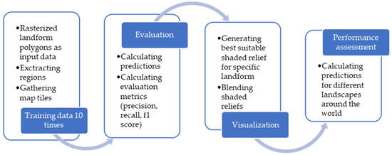
Figure 1.
The workflow.
2.1. Study Area and Data
Given availability of data, we chose to train our model on the territory of Switzerland. We considered deriving source data from several maps such as biogeographical regions, landscape typologies, geomorphology, geology, tectonics, and settlement areas maps. Finally, we extracted the landforms as geomorphological units from the landscape typologies map [16] provided by the Atlas of Switzerland—online (Figure 2).
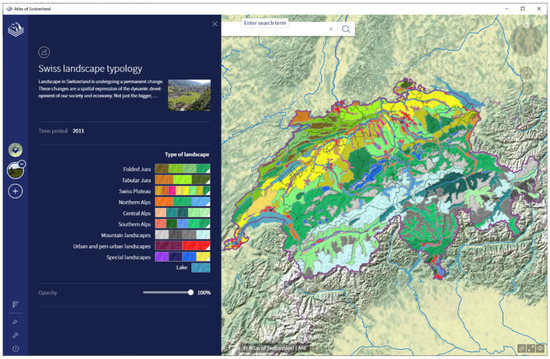
Figure 2.
The Swiss landscape typology map from the Atlas of Switzerland—online [17] © 2022 Atlas of Switzerland.
To match the data with a set of landforms we are interested in [18], we assigned landforms to subtypes of the landscape types above. As a result, we derived the following landforms from these data (Table 2):
Table 2.
Swiss landscape types and assigned landforms.
- block mountains (mountainous landscapes of the Swiss Alps)
- folded mountains (mountainous landscape of the Folded Jura)
- Prealps (mainly limestone mountainous and hilly landscapes of the Swiss Alps)
- plateaus (plateau and hilly landscapes of the Folded and Table Jura)
- erosion (mountain landscape of the Swiss Plateau, including the Napf area)
- hilly (hilly landscapes of the Swiss Plateau, the Folded and Table Jura)
- valleys
- plains
As seen from the table, we included Prealps, i.e., regions lying on the margins of the Alps, primarily on its northern side, and mainly made of limestone, since they comprise a rather large area and form an interim class between hills and mountains in terms of height, generally not exceeding 2500 m. At the same time, such large-scale landforms as glacier, alluvial fans, and drumlins we excluded from this list. Figure 3 demonstrates the resulting image of the eight landforms chosen for training.
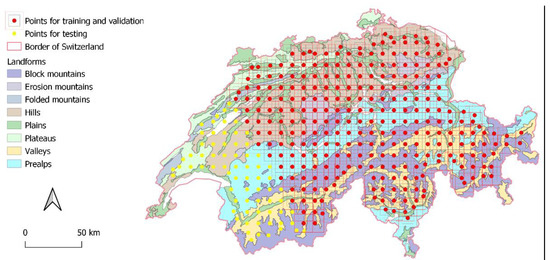
Figure 3.
Landforms extracted from the landscape typology map with training points for training and validation, where both inner (grey) and outer (red) padding borders lie within the Swiss border.
To provide the model with labels, we generated a 10 km grid of regularly distributed training points. Since the model would look as far as the padding areas, we had to make sure all the bounding boxes of 16 km (10 km and a padding of 3 km on both sides) fit completely within the Swiss border, i.e., where ground-truth data are present. For that reason, we manually moved close-to-the-border points away from the border and removed from the dataset those falling outside Switzerland. Out of 357 points, 80% (i.e., 286) of the points we choose for training and validation, while the other 20% of them will serve for the testing purposes (Figure 3). Diagonal cutting of the area ensures the presence of most of the landforms within both training and testing sets.
2.2. Network Architecture
We chose to use a well-established neural network architecture for semantic segmentation, the U-Net [19]. The U-Net, in essence, makes use of a conventional encoder–decoder architecture. During the encoding path of the model, the input image (in the given case, the tile of the DEM) is being gradually transformed into more and more compact feature maps, each representing the input image at an increasing level of abstraction. This is achieved by iteratively applying convolutional layers and max-pooling layers. Hence, the spatial dimensions of the DEM are decreased, while the number of channels is increased. Since the final goal of a segmentation is to provide a classification of each pixel of the DEM, this compact representation needs to be transformed back to the original spatial extents. This is conducted by iteratively applying de-convolutional operations, until the original spatial extents are obtained. Conventional encoder–decoder architectures have the caveat of yielding blurry results. The U-Net architecture circumvents this issue by adding skip connections between layers of the encoder path with layers of the decoder paths that share the same dimension. In essence, those skip connections merge the corresponding feature maps. This way, they can be analyzed in conjunction by subsequent convolutional operations. In practice, the input dimensions of the U-Net (i.e., the area the network “sees”) are larger than the output dimensions (i.e., the area for which pixel classifications should be generated). The reason for this lies in the idea that there is not enough context information for border pixels to be able to create reasonable classifications. Hence, a final cropping operation is applied to remove border pixels for which no meaningful results are expected. Finally, drop out layers are inserted to prevent overfitting, a technique that has been proven useful for similar applications [20]. The final convolutional layer makes use of a softmax activation function. All other activations are set to ReLu.
The original input dimensions of 192 × 192 pixels are reduced to 6 × 6 pixels. However, the number of channels is increased from 1 (i.e., the normalized height) to 128. For the output, we have eight channels, one for each landform, whereas the original U-Net has only two output channels.
The Adam optimizer used for learning and categorical cross entropy is used as a loss function. The number of epochs is set to 2000 and early stopping is used with a patience of 400.
The architecture has the following differences to the original architecture and is therefore more similar to that described in [20]. As with the U-Net architecture of [20], it downsamples the input five times (number of max pooling layers) instead of four times as is done in the original architecture. Additionally, dropout is added to each layer with a constant probability of 0.015 (the original U-Net architecture introduced dropout only for the innermost layers). However, in contrast to the architecture of [20] the input dimensions have been changed from 256 × 256 to 192 × 192. Hence, the innermost representation has the dimensions 6 × 6 instead of 8 × 8 as described in [20]. The number of channels increases from 1 to 128 while [20] compacts to 256 channels in the bottleneck. Because there are eight landforms, the final layer of our U-Net has eight channels (instead of one of the architecture of [20] and two of the original U-Net). Additionally, the authors in [20] deal with a regression problem, while the task of this paper is a classification problem. Hence, we use a SoftMax activation instead of a ReLU activation for the final layer.
2.3. Blending the Shadings Based on the Segmentations
To ensure we blend shaded reliefs without noticeable transitions between them, the following workflow is being used. First, the boundaries of each segmented landform class are being buffered by a user-defined amount. This leads to overlapping areas along the boundaries of these landforms. Then, distance transforms are calculated for the buffered areas, indicating for each pixel how far they are from the buffered boundary. These distance values are then divided by twice the buffer distance. Hence, pixels close to the buffered boundary will be approaching zero while pixels within the original polygon that are twice times the buffer distance afar from the buffered boundary (1 buffer distance afar from the original boundary) will hold the value 1. Values greater than one will be clamped to 1. This is illustrated in Figure 4.
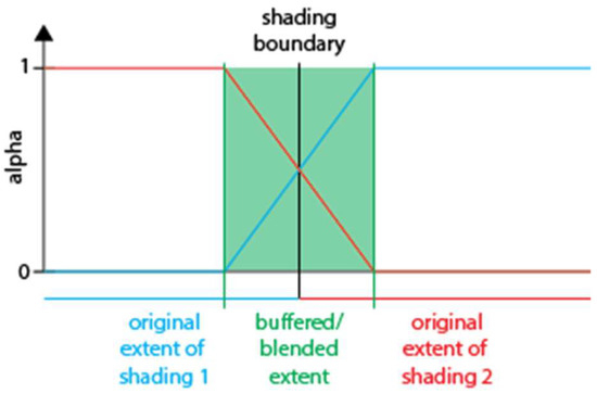
Figure 4.
Construction of the transition area when blending two shadings.
In cases where more than two shadings overlap, normalization of them is being carried out so that all alpha values sum up to 1 for each pixel. Once this is achieved, the different shadings can be blended according to Equation (1):
Here Cblend is the resulting blended grayscale value, αi is the alpha value for a specific landform with index i at that pixel and ci is the grayscale value of the shading of landform i at that pixel, n is the number of landforms.
3. Results
In this section, we provide the training setup and predictions of landforms as the outcome of the training. Furthermore, we assess the performance of the models and the ensemble approach using classification metrics. Finally, we demonstrate how shaded relief can be blended to provide smooth images free from blending artefacts.
3.1. Training
The number of epochs varied from training to training and for the 10 models was in the range of 525–1128 epochs (845, 744, 712, 979, 654, 640, 783, 826, 1128, and 525, respectively) due to early stopping. For 845 epochs, training took approximately 22 h. The setup consists of a NVIDIA GeForce RTX 2080 Ti graphic card, 32GB RAM and an Intel(R) Core(TM) i9-7940X CPU @ 3.10 GHz processor. The neural network is implemented in Keras [21].
Predictions generated based on each of the 10 models, their averaged predictions, and ground-truth data derived from the landscape typology map for comparison are depicted in Figure 5 and Figure 6. All of them display similar landform structure with visible differences at the segmentation boundaries marked in yellow. The ground-truth data (Figure 6b) is more uniform and shows clear boundaries between the landscape types, whereas all the predictions classes look overall more scattered with observable differences mostly in Table and Folded Jura and in the central part of the country. Unlike block mountains or Prealps, the northwestern areas of Switzerland filled with plateaus and folds are much more challenging to delineate. The plateaus of the Table Jura in the northeastern extension of the Jura Mountains are better recognized by all the 10 models, while those of Folded Jura are represented as a mixture of hills, erosion and block mountains. Erosion mountains of the Central Switzerland appear to be largely mixed with hills and even some plateaus, which are absent in the ground-truth data. The same issue also relates to the territories of Appenzell in the northeastern Switzerland. The southern part of Ticino displays a different ratio of plains, hills and plateaus with dominant Prealps around them. In addition, in the valley of the Rhône river in the canton of Valais we can see a different distribution of valleys, plains and Prealps.
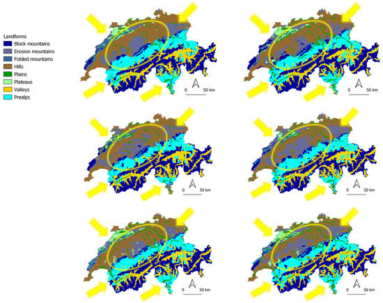
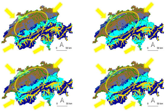
Figure 5.
Predictions of each of the 10 training models with differences marked in yellow.
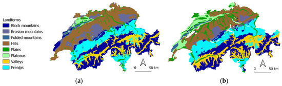
Figure 6.
(a) Average predictions of the 10 models together, (b) ground-truth data.
3.2. Performance Assessment
To evaluate and quantify the quality of predictions, we compute the following classification metrics using the Scikit-learn library [22]—precision, recall, and f1 score [23]:
- Precision gives the proportion of correctly predicted landforms to the total of all positively predicted ones and helps us not to label as correct a landform that is wrong
- Recall returns the proportion of true positives regarding the total number of true positive and false negative results, which basically allows for finding all the correct landforms
- f1 score is a harmonic mean of precision and recall
Confusion matrices in Figure 7 represent the number of true positives, true negatives, false positives, and false negatives for all the models, and Table 3 gives an overview of the original and average evaluation metrics values of each model and the ensemble, as well as their accuracies, which are the metrics that provide a single number for comparison.
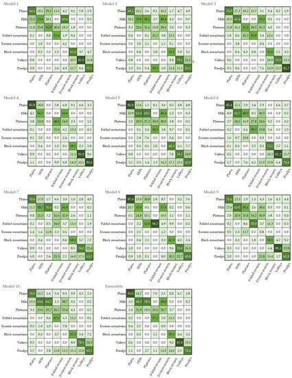
Figure 7.
Confusion matrices for all the models and the ensemble (%). The darker the background of a cell, the higher the value it represents.
Table 3.
Evaluation metrics across the 10 models and the ensemble (%). The darker the background of a cell, the higher the value it represents.
It is not easy to determine the best model, since their predictive power differs heavily among landform classes. Thus, we averaged the predictions of all the models at Table 3 to receive potentially better results than each separate one.
As we can see, the models perform particularly well for block mountains, Prealps, valleys, and hills, with the f1 score in the range of 60% to 70% (Table 3). These landforms together with plains have the highest precision across 10 models, but also rather high recall, which has a noticeable effect on the model accuracy.
The least recognized landforms are erosion mountains, the precision rates for which did not exceed 10% by any model. The models were mostly confused when segmenting plateaus and folded mountains, with the most scattered precision values from 0% to 51.9% for plateaus and from 31.23% to 98.22% for folded mountains, respectively. The reason for such a sharp deviation and low recognition rates is overall much smaller training areas available for folded mountains, plateaus, and erosion mountains in contrast to other landforms (Table 4). For the rest of the landforms the differences in precision values were smaller, and standard deviation of precision across the models is in the range of 3.71–8.51%, as opposed to 17.35% for plateaus and 19.98% for folded mountains.
Table 4.
Areas covered by landforms in Switzerland.
Compared to the average precision values of the 10 models, the ensemble approach (Table 3) delivers significantly better precision for valleys, plains and Prealps and slightly better values for block mountains, folded mountains, and hills. In relation to plateaus and erosion mountains it performs a bit worse, and with respect to accuracy, it outperforms the average accuracy of the models, 61% vs. 57.40%. In the same times, model 6 displayed even higher accuracy of 65%, which allows us to use it further for testing the algorithm within other geographic regions.
3.3. Blending Shaded Reliefs
According to the results of the relief shading user survey [18], Table 5 includes the combinations of relief shading techniques used to blend the shaded reliefs that were segmented by prediction maps.
Table 5.
Combinations of relief shading techniques to apply depending on landform.
Not all the eight landforms are present in the survey, thus we decided to consider hills as drumlins to test two different relief shading techniques. Since there are different survey results for V- and U-shaped valleys, we will consider both types as V-shaped valleys, because it would be impossible to apply custom illumination to every single U-shaped valley within Switzerland, whereas clear sky model is anyway rated second best for U-shaped valleys. Prealps and plains, also absent in the survey, will be rendered using the generally best rated relief shading technique across the landforms, i.e., clear sky model. We blend the shaded relief segmented using the model 6 (Figure 8, Figure 9 and Figure 10), since it demonstrated the highest accuracy of the 10 models and the ensemble. For smooth transitions between the segmented parts, we applied 150 iterations, i.e., a 150 pixel-wide blending zone.
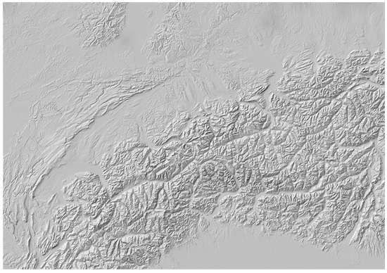
Figure 8.
First-choice blended shaded reliefs.
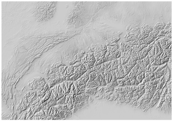
Figure 9.
Second-choice blended shaded reliefs.
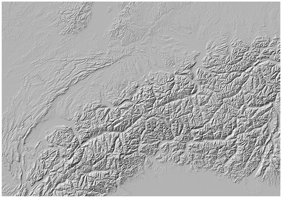
Figure 10.
Traditional analytical relief shading using an illumination source from one direction (315°).
3.4. Testing Areas
To find out whether models and choice of the landforms may also be applied to other mountainous areas around the world, we tested the model on a selection of areas outside Switzerland. The preconditions are the comparable relief in terms of the type and the size of landforms, data in the projected coordinate system, and the same resolution as the input data, i.e., 100 m. Since model 6 has the highest accuracy of all the models and of the ensemble, we generated the predictions based on model 6. Due to the absence of ground-truth data (landscape segmentation boundaries) for these areas, we performed a visual assessment of the resulting predictions. For the testing areas, we chose the Shuttle Radar Topography Mission (SRTM) data available via the USGS EarthExplorer [24]: the Zagros Mountains, the Carpathians, the Ouachita Mountains, and Caucasus (all folded mountains), as well as Sierra Nevada (block mountains).
The Zagros Mountains, located in Iran, northern Iraq and south-eastern Turkey contain multiple landforms we are interested in. It is a long mountain range stretching for 1600 km, and its highest point Mount Dena (4409 m) is in the same range as that of the Alps. The mountains are made primarily of limestone. The central and northern parts of the predictions depict block mountains (those are also the highest areas of the mountain range), and the large areas around them are defined as Prealps (Figure 11). Due to the lower accuracies for plateaus and folded mountains, they mostly appear scattered in the southern part, where the mountains cover the Iranian plateau, though there are many elongated folds that stretch along the folded belt of the plateau [25].
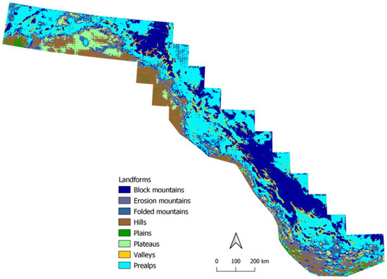
Figure 11.
Predictions for the Zagros Mountains.
The Carpathians are a mountain range in the shape of an arc in the Central and Eastern Europe. It is lower compared to the Alps and has its highest peak of 2655 m in the norther part [26]. Its predictions (Figure 12) appear to change with elevation a lot, and most of the mountainous area are defined as erosion mountains, respectively, due to heights and similar rounded shape. The squared patterns over the plains are caused by tiling, and these artefacts occur, because the model did not “see” large areas of plains in the input dataset.
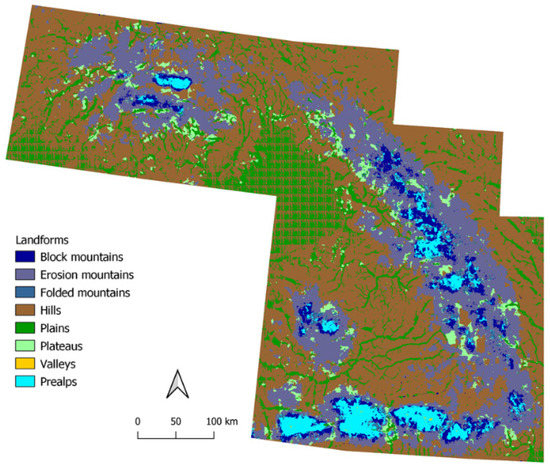
Figure 12.
Predictions for the Carpathian Mountains.
The Ouachita Mountains in the central part of the USA extend approximately 360 km east to west, and approximately 80–95 km north to south with the highest elevation of 839 m. Since it has a high degree of folding, the whole range is divided into subranges, with ridges separated by rather broad valleys [27]. Figure 13 shows that the model was able to segment the valleys between the folds, but the folds themselves it recognized as block mountains and not folds, surrounded by relatively large areas defined as Prealps.
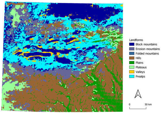
Figure 13.
Predictions for the Ouachita Mountains.
Figure 14 demonstrates the predictions for the Sierra Nevada mountain range in the western United States, which is also a part of the American Cordillera. With the highest elevation of 4421 m, it consists primarily of block mountains, which is also showed by the predictions. The adjacent areas are predicted as Prealps, whereas lower parts neighboring hills depict multiple plateaus. This is due to the presence of table mountains in the area, which were formed by lava that filled some of the canyons, which in turn eroded and left table mountains instead [28].
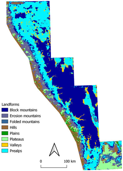
Figure 14.
Predictions for the Sierra Nevada mountain range.
Lastly, Figure 15 shows the predictions for the Caucasus Mountains. Its highest peak Mount Elbrus is at 5642 m [29], and the vast predictions area depict the block mountains, valleys carved into the mountains and lower areas corresponding to Prealps. The model could also predict plateau areas in the foothills of the main range.
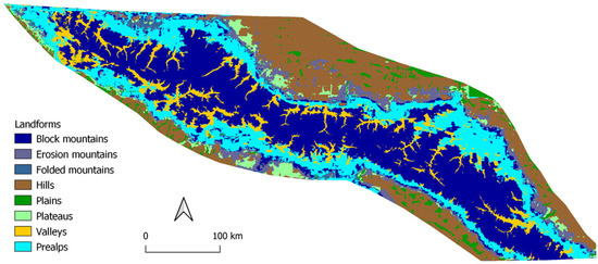
Figure 15.
Predictions for the Caucasus Mountains.
As we can see, the predictions created for testing areas bring us a basic picture and understanding of those mountainous structures. Given the received accuracy, we cannot expect near ground-truth results, but there is definitely a potential for increasing the quality of predictions by improving the whole network, training more models, or choosing the best performing model for a certain landform, e.g., model 8 for folded mountains or model 9 for valleys.
4. Discussion
The presented experiments showcase several challenges which must be overcome so that a reliable landform recognition and terrain segmentation for the purpose of relief shading is obtained. First, a clear definition of landforms needs to be created that would allow machine-learning models to infer the correct landform from a small set of input data, ideally only DEM. This issue becomes particularly obvious when using a simple definition of a valley and a ridge: If one defines a valley as “an area between two ridges” and a ridge as “an area between two valleys”, both feature classes would nearly entirely overlap. Such a case makes segmentation unfeasible in the first place. So where does one draw the boundary between different landforms? Along with this question comes the implication whether different landforms can actually overlap, e.g., whether a single hill on a plateau belongs to both the plateau class and the hill class. This again might have an impact on the neural network architecture to be used.
Second, due to computational limitations, neural networks only have a limited “field of view”, i.e., the area they can take into account to make a prediction. Consequently, this limits their use to classify landforms that cover large extents, as they likely cannot be analyzed as a whole. This is directly linked with the influence of the resolution of the input data, predominantly DEM. The lower the resolution, the further a neural network can “see” in terms of the geospatial extent. Hence, for small landforms, a higher resolution might be beneficial, while a lower resolution might be more advantageous to carry out segmentation for larger landforms. This challenge will likely vanish with the ongoing advancement of computer hardware.
Third, we only investigated a standard U-Net architecture to perform landform segmentation. However, many different flavors of the U-Net [30] or entirely different architectures exist for segmentation (e.g., [31,32,33,34]). A comparison of different architectures is likely a worthwhile endeavor.
It is also important to mention that the input data, i.e., the landscape typology map, was made manually by humans and an improved and more accurate classification could also deliver better results and make them more consistent. A potentially more accurate input data other than man-made maps could also be information about the soil and bedrock compositions, satellite imagery, or probably also information about surface features such as rivers, building, etc. And yet we would need a more precise manually labeled map about the geomorphological features.
Furthermore, there are certain limitations regarding the recognition rates of the landforms. First, some landforms such as erosion mountains are in itself more challenging to recognize or classify due to their visual similarity with hilly areas. Additionally, there are also similar-looking places within hills, Prealps, and plateaus areas that cannot always be successfully distinguished from one another. In addition, in this approach we used a regular grid of training points, and a very different number of points fell within different landforms. At the same time, some landforms cover much larger areas than the others do. For example, the area covered by block mountains is more than 10 times larger than that covered by folded mountains (Table 4). As a result, the training cannot be equally efficient for all the landforms. Finally, there is an unpredictability on the subject of training: from one model to another, there might be very different results, i.e., one model may recognize plateaus, for instance, while another not at all.
5. Conclusions
In this work, we proposed a novel approach to segment terrain by applying adapted U-Net architecture with the aim to subsequently improve the quality of relief shading applied to segmented areas. Quantitative assessment revealed the highest precision value of 89.33% for valleys and 81.71% for Prealps. For block mountains and hills, precision values reached 72.06% and 63.58%, respectively, and for folded mountains and plateaus, the values are more scattered and vary from 31.23% to 98.22% and from 0% to 51.90% due to smaller areas being available for testing. The average accuracy across 10 models is 57.40%, and one of the models reached accuracy of 65%, whereas the ensemble approach did not manage to outperform single models and delivered the accuracy of 61%. Though there is room for enhancement, e.g., regarding the accuracies of the models, our approach proved to be effective when it comes to such landforms as block mountains, Prealps, valleys, and hills, which delivered well readable segmentations of testing areas outside of the area on which we tested our network.
Author Contributions
Conceptualization, Marianna Farmakis-Serebryakova, Magnus Heitzler and Lorenz Hurni; Data curation, Marianna Farmakis-Serebryakova and Magnus Heitzler; Formal analysis, Marianna Farmakis-Serebryakova and Magnus Heitzler; Investigation, Marianna Farmakis-Serebryakova and Magnus Heitzler; Methodology, Marianna Farmakis-Serebryakova, Magnus Heitzler and Lorenz Hurni; Resources, Marianna Farmakis-Serebryakova, Magnus Heitzler and Lorenz Hurni; Software, Marianna Farmakis-Serebryakova and Magnus Heitzler; Supervision, Marianna Farmakis-Serebryakova, Magnus Heitzler and Lorenz Hurni; Validation, Marianna Farmakis-Serebryakova and Magnus Heitzler; Visualization, Marianna Farmakis-Serebryakova; Writing—original draft, Marianna Farmakis-Serebryakova; Writing—review and editing, Marianna Farmakis-Serebryakova, Magnus Heitzler and Lorenz Hurni. All authors have read and agreed to the published version of the manuscript.
Funding
This research received no external funding.
Institutional Review Board Statement
Not applicable.
Informed Consent Statement
Not applicable.
Data Availability Statement
Data ownership lies with Swisstopo and the Atlas of Switzerland, hence data cannot be published alongside the paper.
Acknowledgments
The authors would like to thank the editors for their valuable feedback and suggestions.
Conflicts of Interest
The authors declare no conflict of interest.
References
- Schmidt, J.; Andrew, R. Multi-scale landform characterization. Area 2005, 37, 341–350. [Google Scholar] [CrossRef]
- Drăguţ, L.; Blaschke, T. Automated classification of landform elements using object-based image analysis. Geomorphology 2006, 81, 330–344. [Google Scholar] [CrossRef]
- Drăguţ, L.; Eisank, C. Automated object-based classification of topography from SRTM data. Geomorphology 2012, 141, 21–33. [Google Scholar] [CrossRef] [PubMed] [Green Version]
- Liu, S.; Li, F. A method of automatic topographic recognition based on slope spectrum. Geomorphometry Geosci. 2015, 129–132. Available online: https://geomorphometry.org/wp-content/uploads/2021/07/Liu2015geomorphometry.pdf (accessed on 30 April 2022).
- Buscombe, D.; Ritchie, A.C. Landscape classification with deep neural networks. Geosciences 2018, 8, 244. [Google Scholar] [CrossRef] [Green Version]
- Mohammadimanesh, F.; Salehi, B.; Mahdianpari, M.; Gill, E.; Molinier, M. A new fully convolutional neural network for semantic segmentation of polarimetric SAR imagery in complex land cover ecosystem. ISPRS J. Photogramm. Remote Sens. 2019, 151, 223–236. [Google Scholar] [CrossRef]
- Bhuiyan, M.A.E.; Witharana, C.; Liljedahl, A.K.; Jones, B.M.; Daanen, R.; Epstein, H.E.; Kent, K.; Griffin, C.G.; Agnew, A. Understanding the effects of optimal combination of spectral bands on deep learning model predictions: A case study based on permafrost Tundra landform mapping using high resolution multispectral satellite imagery. J. Imaging 2020, 6, 97. [Google Scholar] [CrossRef] [PubMed]
- Saah, D.; Tenneson, K.; Poortinga, A.; Nguyen, Q.; Chishtie, F.; Aung, K.S.; Markert, K.N.; Clinton, N.; Anderson, E.R.; Cutter, P.; et al. Primitives as building blocks for constructing land cover maps. Int. J. Appl. Earth Obs. Geoinf. 2020, 85, 101979. [Google Scholar] [CrossRef]
- Du, L.; You, X.; Li, K.; Meng, L.; Cheng, G.; Xiong, L.; Wang, G. Multi-modal deep learning for landform recognition. ISPRS J. Photogramm. Remote Sens. 2019, 158, 63–75. [Google Scholar] [CrossRef]
- Li, S.; Xiong, L.; Tang, G.; Strobl, J. Deep learning-based approach for landform classification from integrated data sources of digital elevation model and imagery. Geomorphology 2020, 354, 107045. [Google Scholar] [CrossRef]
- Zhao, W.-F.; Xiong, L.-Y.; Ding, H.; Tang, G.-A. Automatic recognition of loess landforms using Random Forest method. J. Mt. Sci. 2017, 14, 885–897. [Google Scholar] [CrossRef]
- Iwahashi, J.; Pike, R.J. Automated classifications of topography from DEMs by an unsupervised nested-means algorithm and a three-part geometric signature. Geomorphology 2007, 86, 409–440. [Google Scholar] [CrossRef]
- Valentine, A.P.; Kalnins, L.M.; Trampert, J. Discovery and analysis of topographic features using learning algorithms: A seamount case study. Geophys. Res. Lett. 2013, 40, 3048–3054. [Google Scholar] [CrossRef] [Green Version]
- Steffen, I. Artificial Intelligence for Landform Recognition; Geomatics Seminar Report; ETH Zurich: Zurich, Switzerland, 2020. [Google Scholar]
- Catani, F. Landslide detection by deep learning of non-nadiral and crowdsourced optical images. Landslides 2021, 18, 1025–1044. [Google Scholar] [CrossRef]
- Landschaftstypologie Schweiz. Available online: https://www.are.admin.ch/are/de/home/laendliche-raeume-und-berggebiete/grundlagen-und-daten/landschaftstypologie-schweiz.html (accessed on 30 April 2022).
- Atlas of Switzerland-Online. Available online: https://www.atlasderschweiz.ch/swiss-landscape-typology/ (accessed on 19 April 2022).
- Farmakis-Serebryakova, M.; Hurni, L. Comparison of relief shading techniques applied to landforms. ISPRS Int. J. Geo-Inf. 2020, 9, 253. [Google Scholar] [CrossRef] [Green Version]
- Ronneberger, O.; Fischer, P.; Brox, T. U-Net: Convolutional networks for biomedical image segmentation. In Medical Image Computing and Computer-Assisted Intervention 2015; Navab, N., Hornegger, J., Wells, W.M., Frangi, A.F., Eds.; Springer: Cham, Switzerland, 2015; pp. 234–241. [Google Scholar] [CrossRef] [Green Version]
- Jenny, B.; Heitzler, M.; Singh, D.; Farmakis-Serebryakova, M.; Liu, J.C.; Hurni, L. Cartographic relief shading with neural networks. IEEE Trans. Vis. Comput. Graph. 2020, 27, 1225–1235. [Google Scholar] [CrossRef] [PubMed]
- Keras. Available online: https://keras.io/about/ (accessed on 30 April 2022).
- Pedregosa, F.; Varoquaux, G.; Gramfort, A.; Michel, V.; Thirion, B.; Grisel, O.; Blondel, M.; Prettenhofer, P.; Weiss, R.; Duchesnay, E.; et al. Scikit-learn: Machine learning in Python. J. Mach. Learn. Res. 2011, 12, 2825–2830. [Google Scholar] [CrossRef]
- Scikit-Learn. Machine Learning in Python. Available online: https://scikit-learn.org/stable/index.html (accessed on 30 April 2022).
- USGS Earth Explorer. Available online: https://earthexplorer.usgs.gov/ (accessed on 30 April 2022).
- Zagros Mountains. Available online: https://en.wikipedia.org/wiki/Zagros_Mountains (accessed on 30 April 2022).
- Carpathian Mountains. Available online: https://en.wikipedia.org/wiki/Carpathian_Mountains (accessed on 30 April 2022).
- Ouachita Mountains. Available online: https://en.wikipedia.org/wiki/Ouachita_Mountains (accessed on 30 April 2022).
- Sierra Nevada. Available online: https://en.wikipedia.org/wiki/Sierra_Nevada (accessed on 30 April 2022).
- Caucasus Mountains. Available online: https://en.wikipedia.org/wiki/Caucasus (accessed on 30 April 2022).
- Wu, S.; Heitzler, M.; Hurni, L. Leveraging uncertainty estimation and spatial pyramid pooling for extracting hydrological features from scanned historical topographic maps. GIScience Remote Sens. 2022, 59, 200–214. [Google Scholar] [CrossRef]
- Yu, C.; Wang, J.; Peng, C.; Gao, C.; Yu, G.; Sang, N. BiSeNet: Bilateral segmentation network for real-time semantic segmentation. In Proceedings of the European Conference on Computer Vision (ECCV), Munich, Germany, 8–14 September 2018. [Google Scholar] [CrossRef]
- Badrinarayanan, V.; Kendall, A.; Cipolla, R. SegNet: A deep convolutional encoder-decoder architecture for image segmentation. IEEE Trans. Pattern Anal. Mach. Intell. 2017, 39, 2481–2495. [Google Scholar] [CrossRef] [PubMed]
- Wu, H.; Zhang, J.; Huang, K.; Liang, K.; Yu, Y. FastFCN: Rethinking dilated convolution in the backbone for semantic segmentation. arXiv 2019, arXiv:1903.11816. [Google Scholar] [CrossRef]
- Takikawa, T.; Acuna, D.; Jampani, V.; Fidler, S. Gated-SCNN: Gated shape CNNs for semantic segmentation. In Proceedings of the 2019 IEEE/CVF International Conference on Computer Vision (ICCV), Seoul, Korea, 27 October–2 November 2019. [Google Scholar]
Publisher’s Note: MDPI stays neutral with regard to jurisdictional claims in published maps and institutional affiliations. |
© 2022 by the authors. Licensee MDPI, Basel, Switzerland. This article is an open access article distributed under the terms and conditions of the Creative Commons Attribution (CC BY) license (https://creativecommons.org/licenses/by/4.0/).