
Landslide Susceptibility Mapping Using Machine Learning: A Danish Case Study

 and
and 
Abstract
:1. Introduction
1.1. Landslide Susceptibility Mapping
1.2. Problem Statement and Study Objectives
- (1)
- How well can well-established machine learning algorithms be employed for landslide susceptibility mapping given the low-lying flat landscape of Denmark?
- (2)
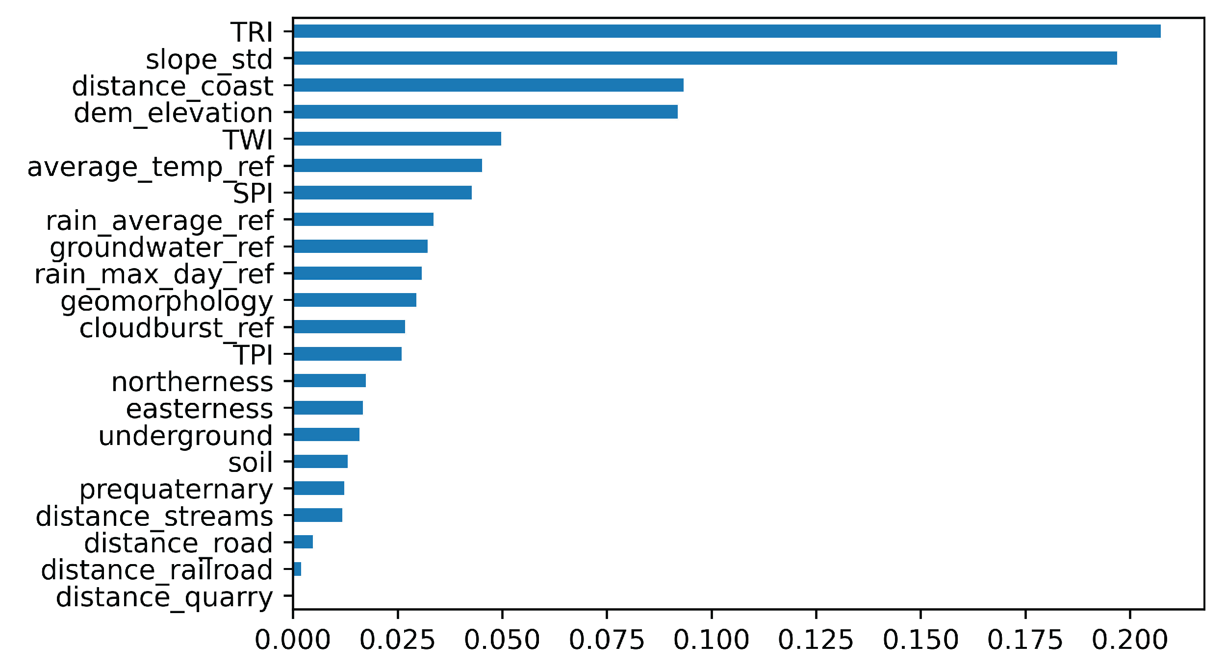
- How are the various variables related to the landslide presence locations? What is the importance of the different variables in the prediction model?
- (3)
- Can the impact of changing climate on landslide susceptibility be modelled for the future climate scenario?
2. Data and Materials
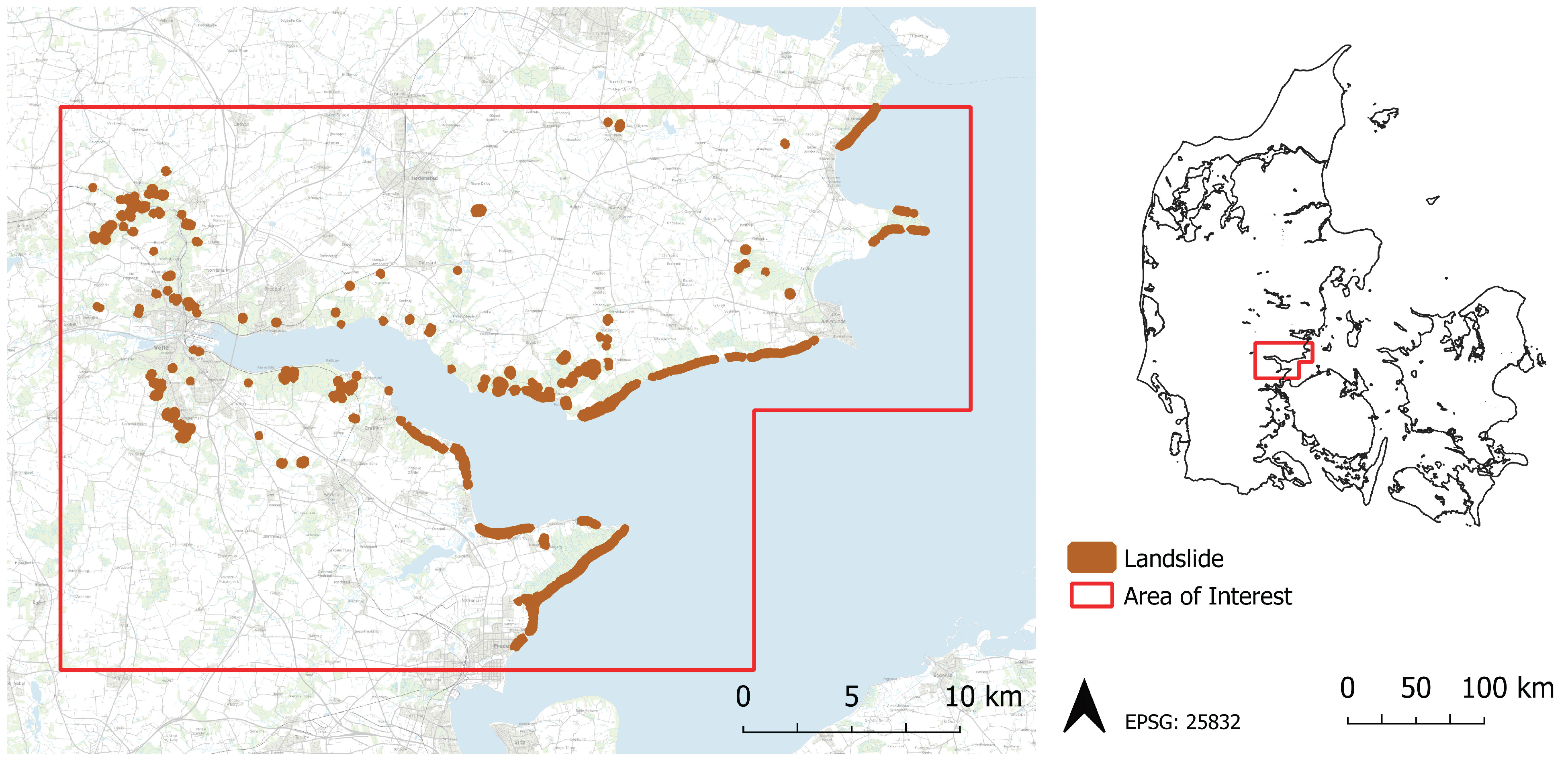
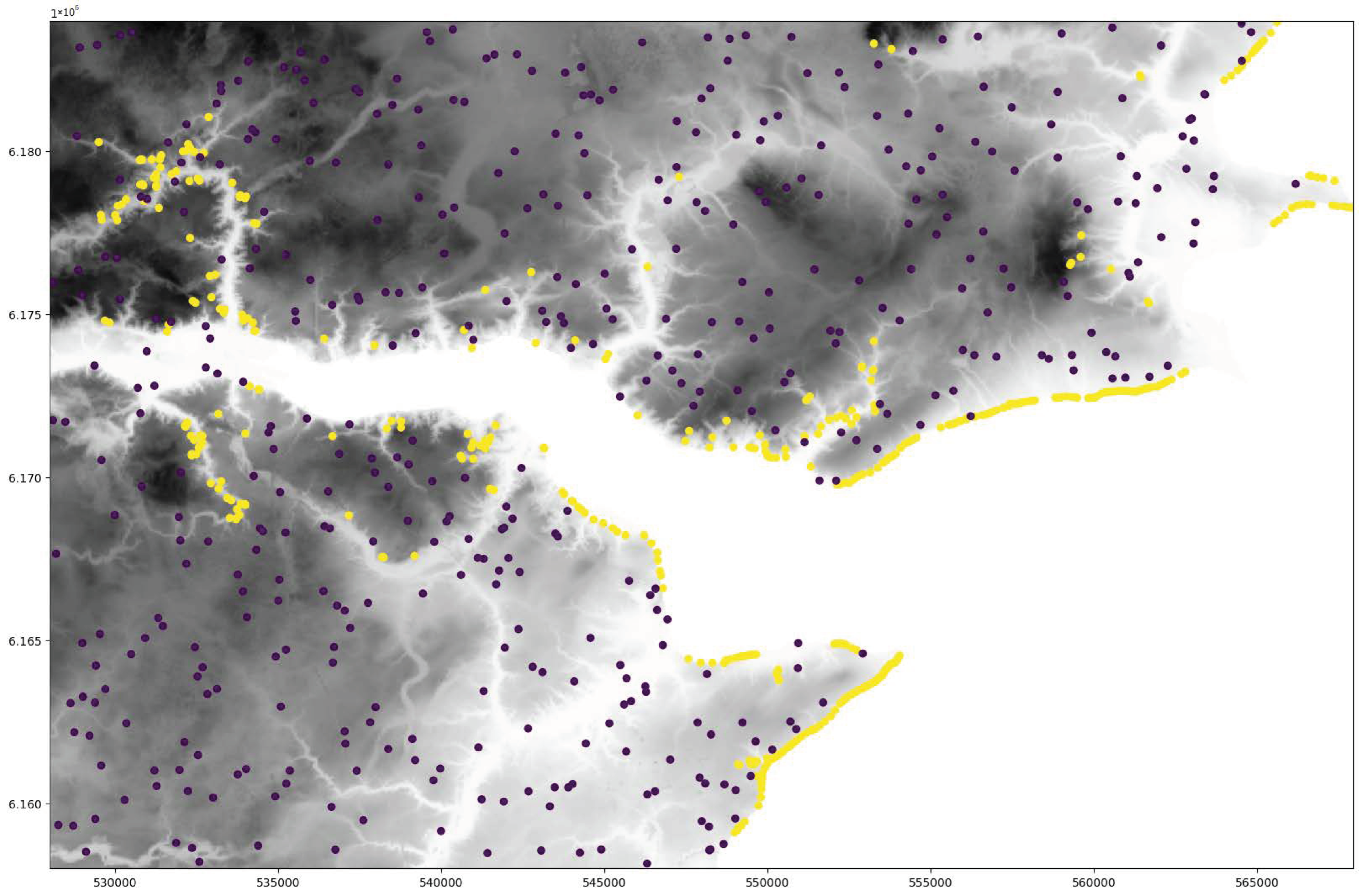
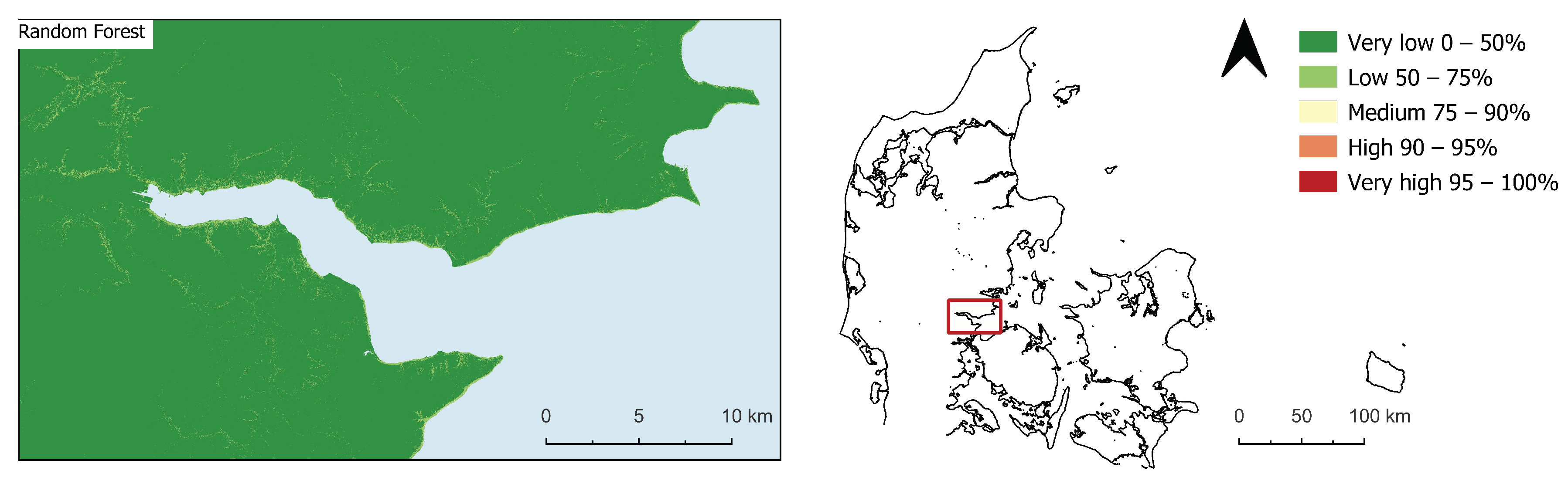
2.1. Area of Interest
2.2. Landslide Inventory
2.3. Predictive Variables
2.4. Climate Data—Present and Future
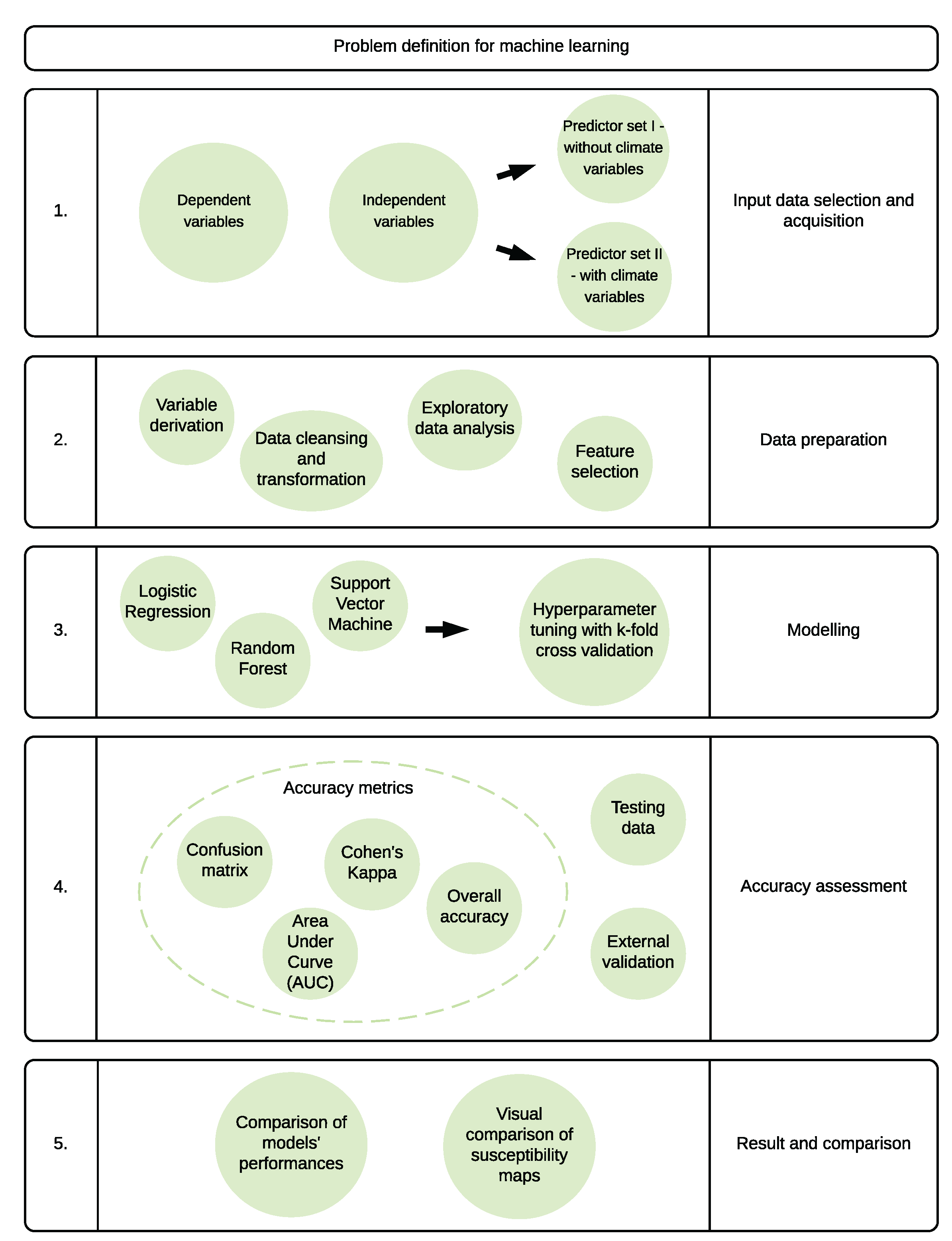
3. Methods
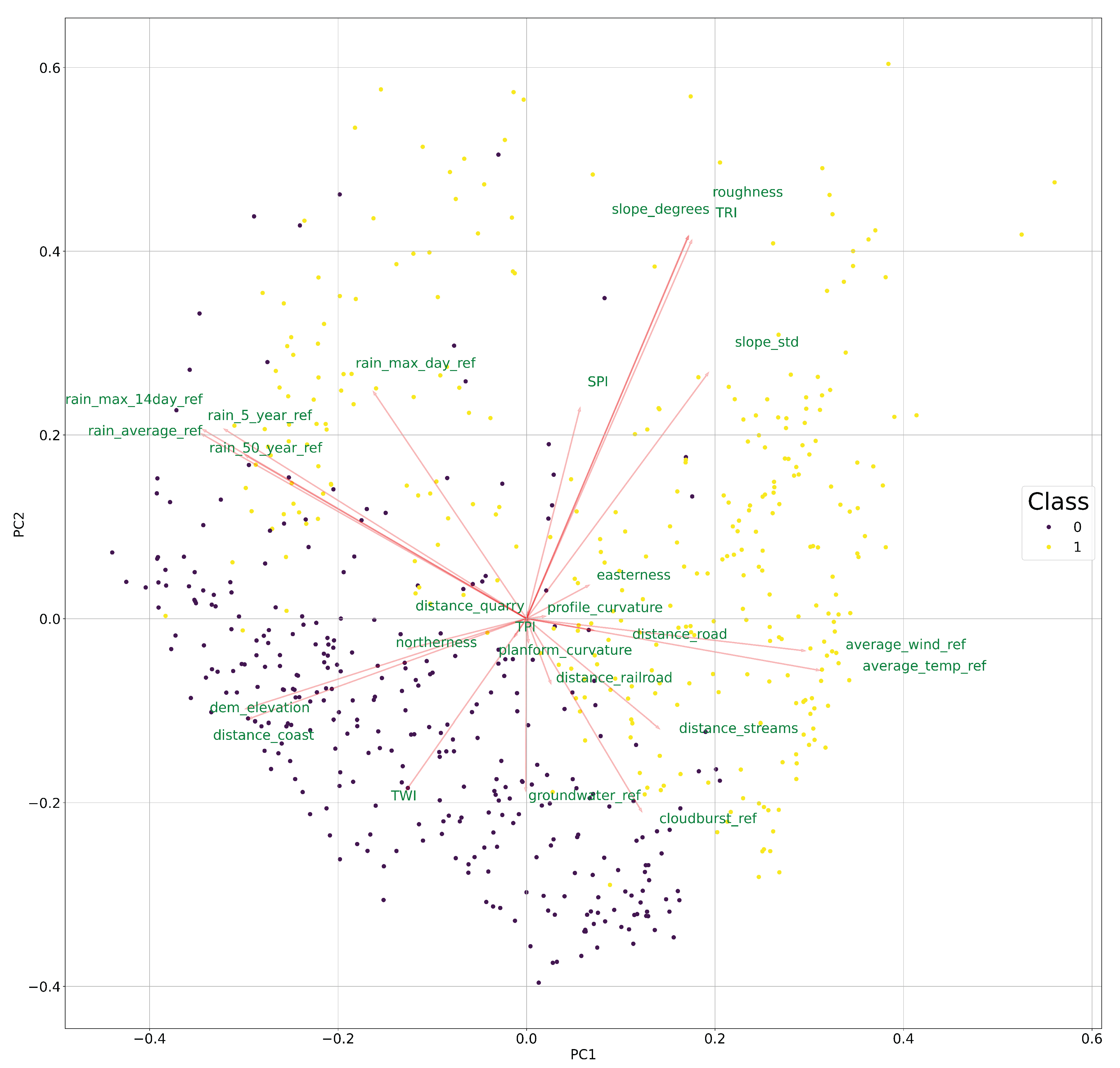
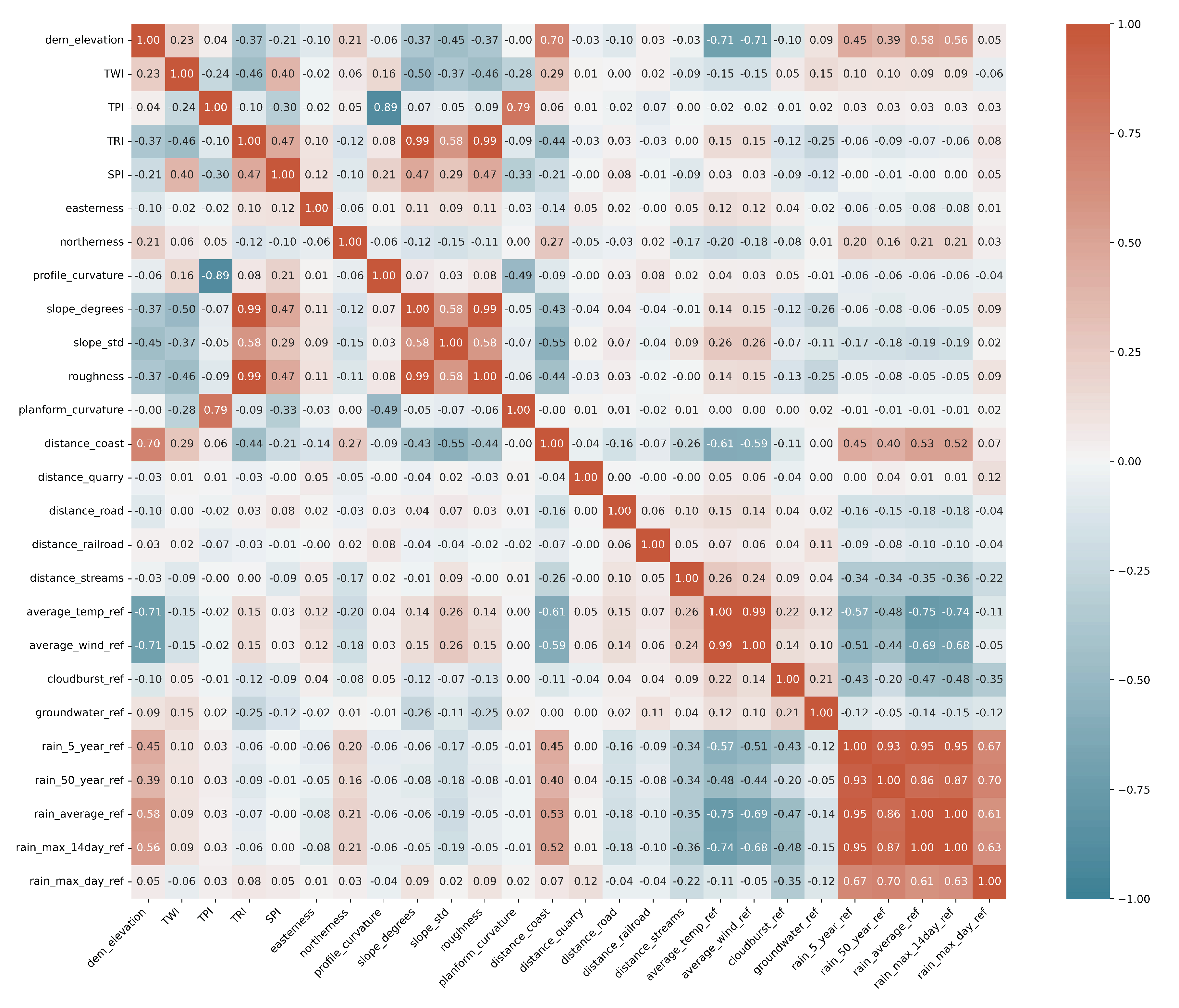
3.1. Feature Selection
- Slope degrees;
- Roughness;
- planform_curvature;
- profile_curvature;
- average_wind_ref;
- rain_max_14day_ref;
- rain_5_year_ref;
- rain_50_year_ref.
3.2. Landslide Susceptibility Modelling: Set Up and Tuning
3.2.1. Random Forest
3.2.2. Support Vector Machine
3.2.3. Logistic Regression
3.3. Hyperparameter Tuning and K-Fold Validation
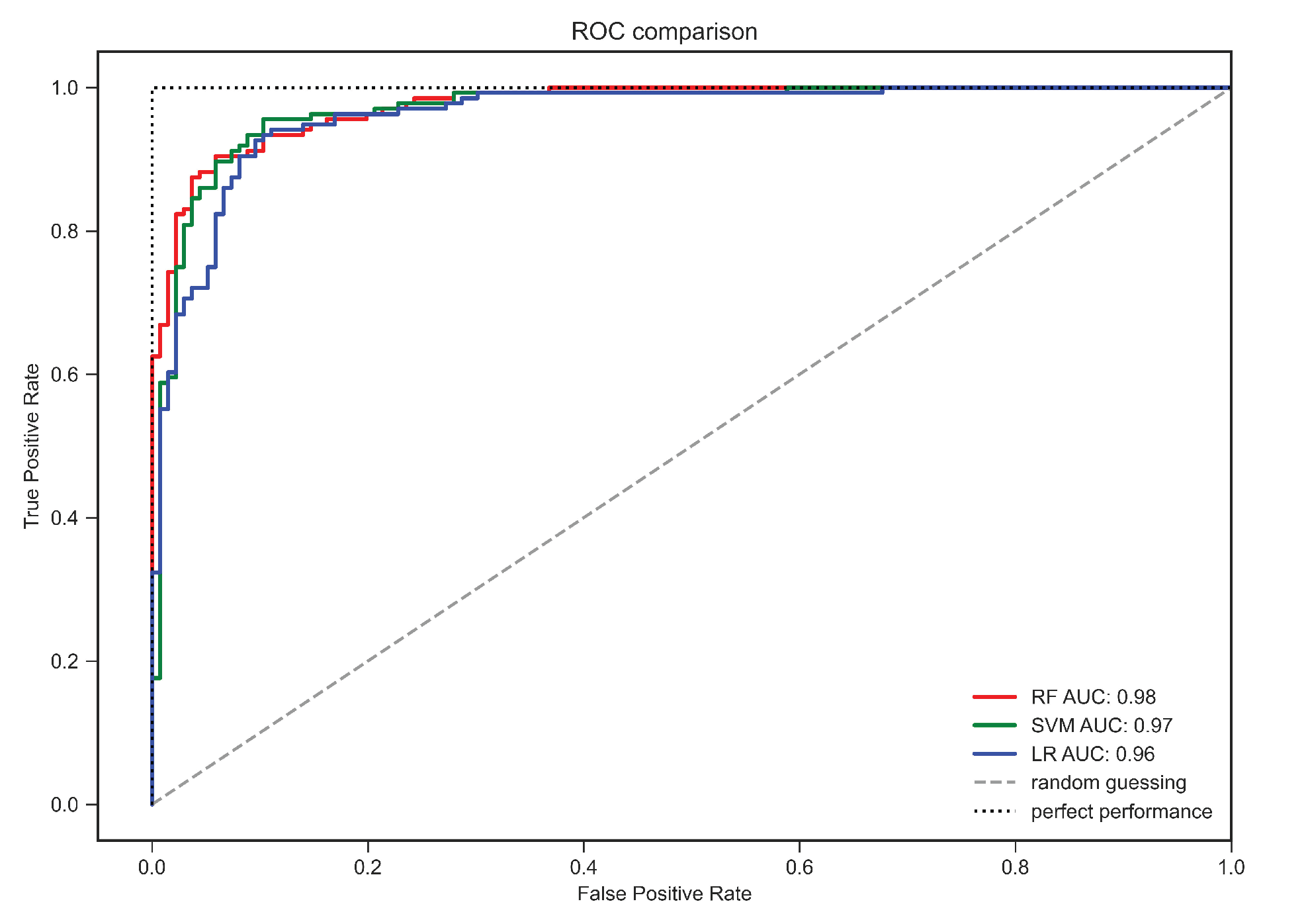
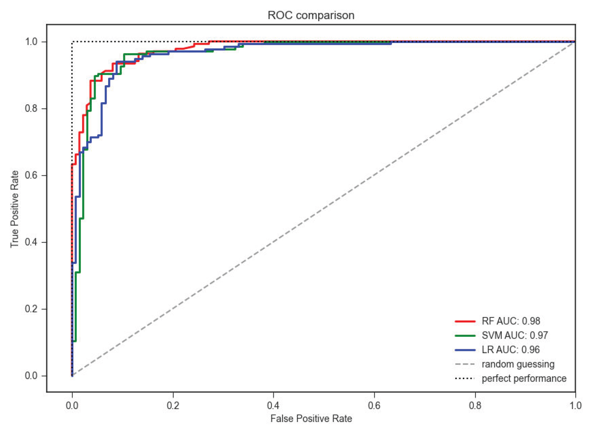
3.4. Accuracy Assessment
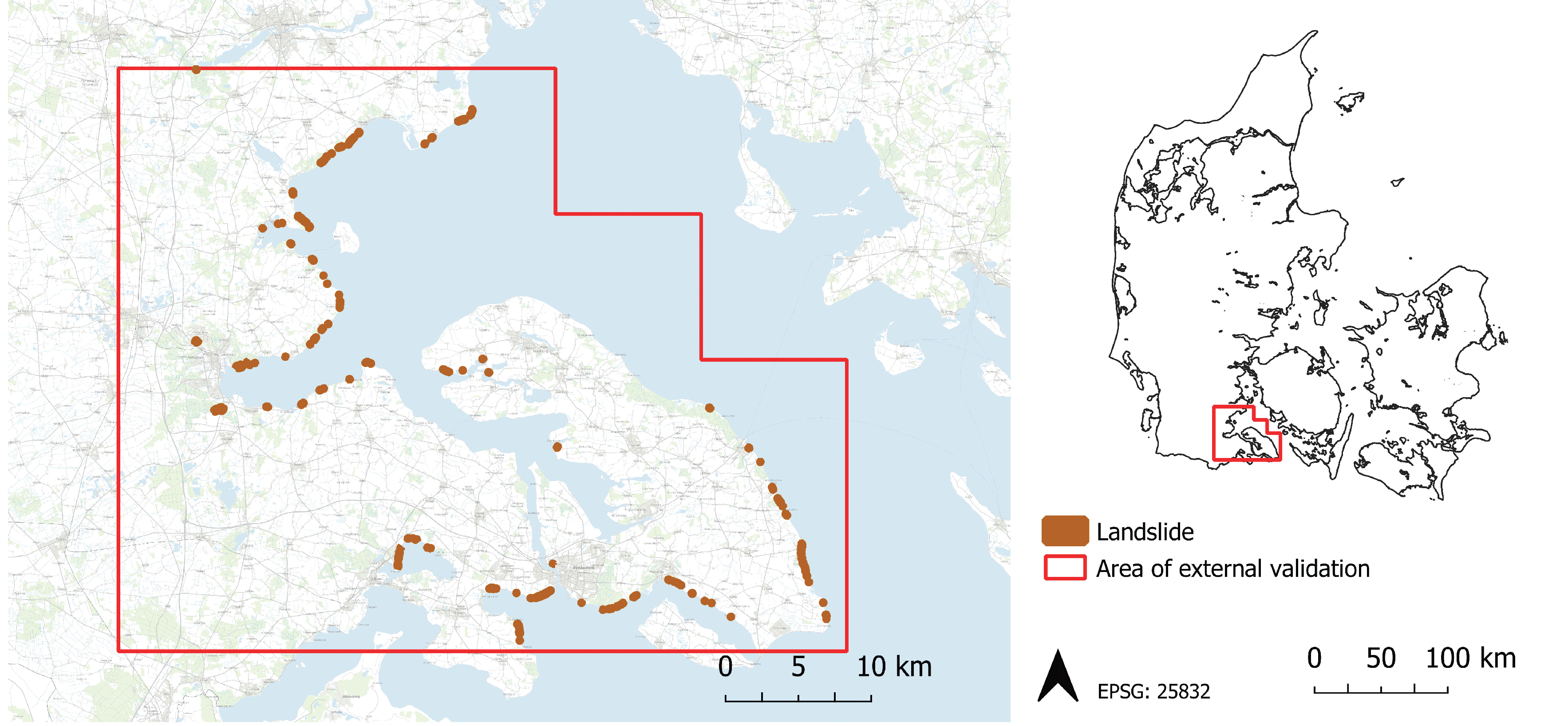
3.5. External Validation
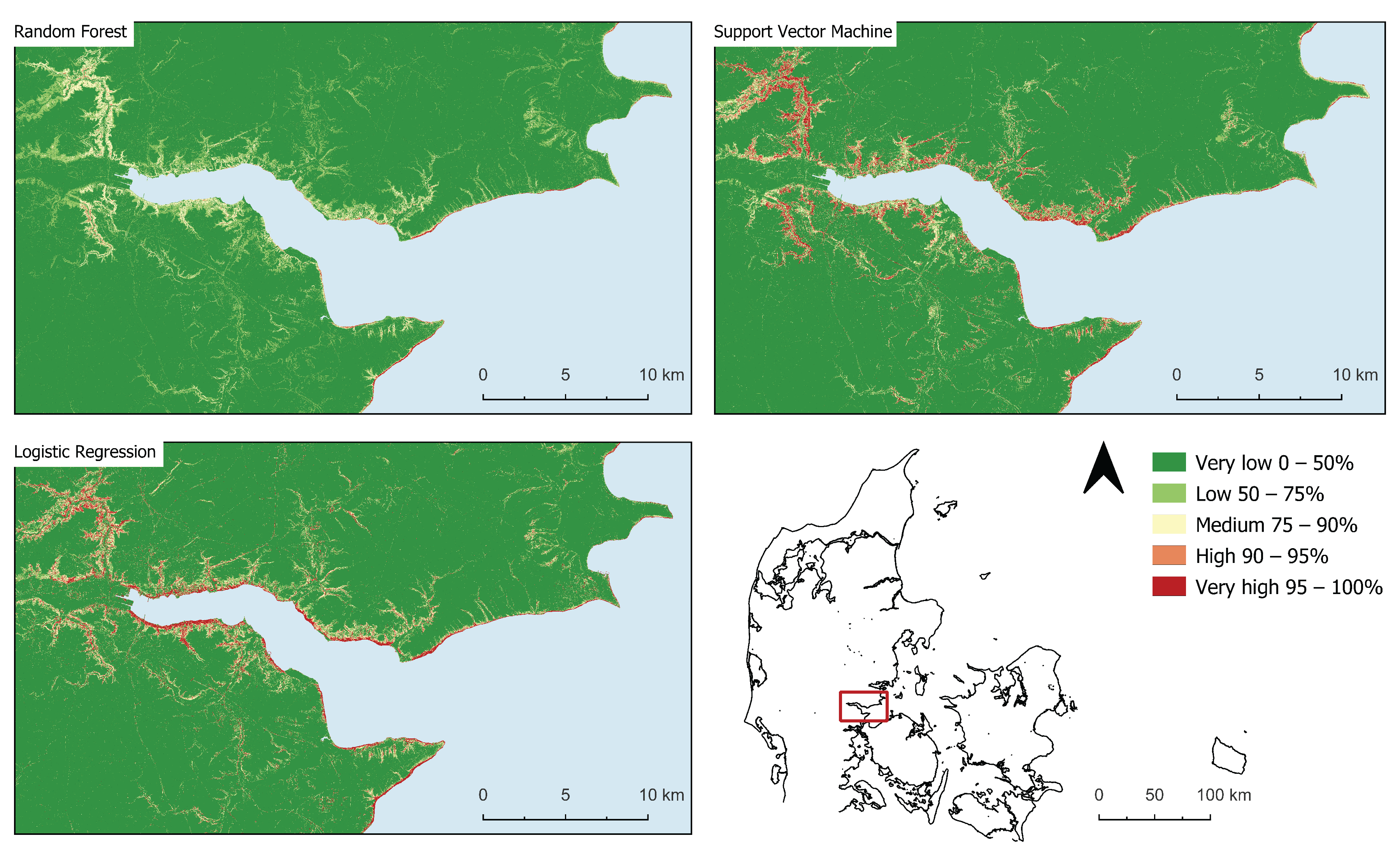
4. Results
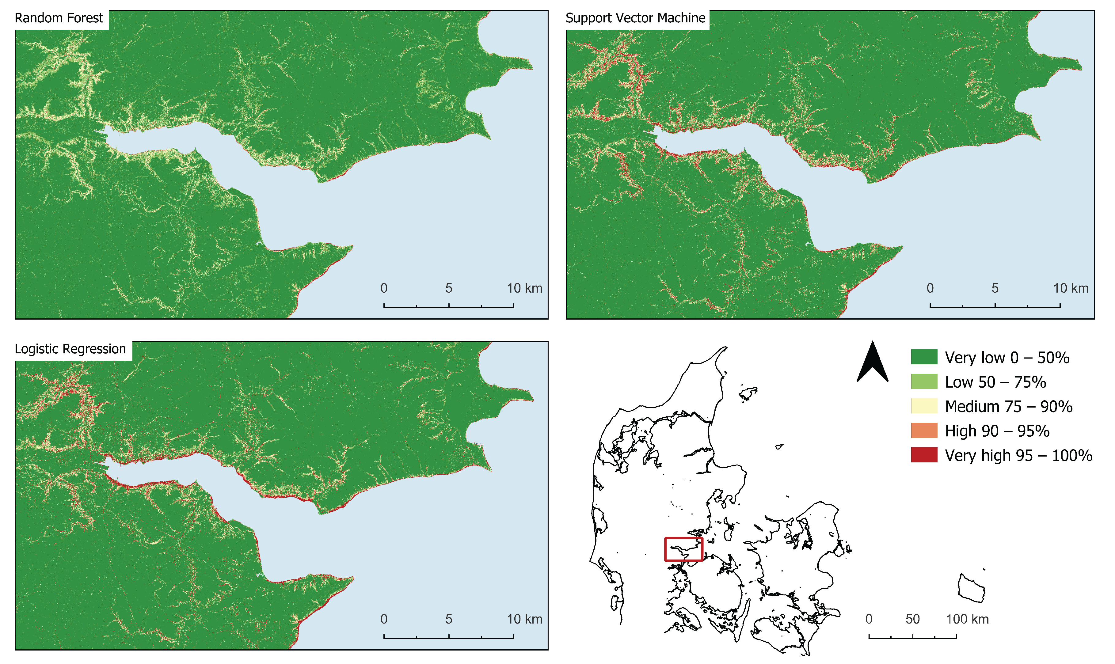
Susceptibility Maps
- distance_coast;
- groundwater;
- cloudburst;
- rain_max_day;
- rain_average;
- average_temp.
5. Discussion
6. Conclusions
Author Contributions
Funding
Institutional Review Board Statement
Informed Consent Statement
Data Availability Statement
Acknowledgments
Conflicts of Interest
References
- Highland, L.M.; Bobrowsky, P. The Landslide Handbook—A Guide to Understanding Landslides, 1st ed.; U.S. Geological Survey Circular 1325: Reston, VA, USA, 2008. [Google Scholar]
- Wallemacq, P.; House, R. Economic Losses, Poverty and Disasters 1998–2017; Centre for Research on the Epidemiology of Disasters, United Nations Office for Disaster Risk Reduction: Geneva, Switzerland, 2018. [Google Scholar]
- Svennevig, K.; Lützenburg, G.; Keiding, M.K.; Pedersen, S.A.S. Preliminary landslide mapping in Denmark indicates an underestimated geohazard. GEUS Bull. 2020, 44. [Google Scholar] [CrossRef]
- Herrera, G.; Mateos, R.M.; García-Davalillo, J.C.; Grandjean, G.; Poyiadji, E.; Maftei, R.; Filipciuc, T.C.; Jemec Auflič, M.; Jež, J.; Podolszki, L. Landslide databases in the Geological Surveys of Europe. Landslides 2017, 15, 359–379. [Google Scholar] [CrossRef]
- Denmark’s Height Model—Terrain. Available online: https://dataforsyningen.dk/data/930 (accessed on 10 May 2022).
- Luetzenburg, G.; Svennevig, K.; Bjørk, A.A.; Keiding, M.; Kroon, A. A national landslide inventory of Denmark. Earth Syst. Sci. Data Discuss. 2021, 1–13. under review. [Google Scholar]
- Field, C.B.; Barros, V.; Stocker, T.F.; Qin, D.; Dokken, D.J.; Ebi, K.L.; Mastrandrea, M.D. Managing the Risks of Extreme Events and Disasters to Advance Climate Change Adaptation; IPCC: Geneva, Switzerland; Cambridge University Press: Cambridge, UK, 2012. [Google Scholar]
- Crozier, M.J. Deciphering the effect of climate change on landslide activity: A review. Geomorphology 2010, 124, 260–267. [Google Scholar] [CrossRef]
- Glade, T.; Crozier, M.J. The nature of landslide hazard impact. In Landslide Hazard and Risk; John Wiley & Sons: Hoboken, NJ, USA, 2005; pp. 43–74. [Google Scholar]
- Camera, C.A.S.; Bajni, G.; Corno, I.; Raffa, M.; Stevenazzi, S.; Apuani, T. Introducing intense rainfall and snowmelt variables to implement a process-related non-stationary shallow landslide susceptibility analysis. Sci. Total Environ. 2021, 786, 147360. [Google Scholar] [CrossRef]
- Dikshit, A.; Sarkar, R.; Pradhan, B.; Ratiranjan, J.; Dowchu, D.; Alamri, A. Probability Assessment and Its Use in Landslide Susceptibility Mapping for Eastern Bhutan. Water 2020, 12, 267. [Google Scholar] [CrossRef] [Green Version]
- Lin, Q.; Lima, P.; Steger, S.; Glade, T.; Jiang, T.; Zhang, J.; Liu, T.; Wang, Y. National-scale data-driven rainfall induced landslide susceptibility mapping for China by accounting for incomplete landslide data. Geosci. Front. 2021, 12, 267. [Google Scholar] [CrossRef]
- Roy, J.; Saha, S. Landslide susceptibility mapping using knowledge driven statistical models in Darjeeling District, West Bengal, India. Geoenviron. Disasters 2019, 6, 1–18. [Google Scholar] [CrossRef] [Green Version]
- Malka, A. Landslide susceptibility mapping of Gdynia using geographic information system-based statistical models. Nat Hazards 2021, 107, 639–674. [Google Scholar] [CrossRef]
- Wu, C. Landslide Susceptibility Based on Extreme Rainfall-Induced Landslide Inventories and the Following Landslide Evolution. Water 2019, 11, 2609. [Google Scholar] [CrossRef] [Green Version]
- Nam, K.; Wang, F. An extreme rainfall-induced landslide susceptibility assessment using autoencoder combined with random forest in Shimane Prefecture, Japan. Geoenviron. Disasters 2020, 7, 1–16. [Google Scholar] [CrossRef] [Green Version]
- Huang, F.; Zhang, J.; Zhou, C.; Wang, Y.; Huang, J.; Zhu, L. A deep learning algorithm using a fully connected sparse autoencoder neural network for landslide susceptibility prediction. Landslides 2020, 17, 217–229. [Google Scholar] [CrossRef]
- Bernardie, S.; Vandromme, R.; Thiery, Y.; Houet, T.; Gremont, M.; Masson, F.; Grandjean, G.; Bouroullec, I. Modelling landslide hazards under global changes: The case of a Pyrenean valley. Nat. Hazards Earth Syst. Sci. 2021, 21, 147–169. [Google Scholar] [CrossRef]
- Kim, H.G.; Lee, D.K.; Park, C.; Kil, S.; Son, Y.; Park, J.H. Evaluating landslide hazards using RCP 4.5 and 8.5 scenarios. Environ. Earth Sci. 2015, 73, 1385–1400. [Google Scholar] [CrossRef]
- Gassner, C.; Promper, C.; Beguería, S.; Glade, T. Climate Change Impact for Spatial Landslide Susceptibility. In Engineering Geology for Society and Territory—Volume 1; Lollino, G., Manconi, A., Clague, J., Shan, W., Chiarle, M., Eds.; Springer: Cham, Switzerland, 2015. [Google Scholar]
- Shou, K.J.; Yang, C.M. Predictive analysis of landslide susceptibility under climate change conditions—A study on the Chingshui River Watershed of Taiwan. Eng. Geol. 2015, 192, 46–62. [Google Scholar] [CrossRef]
- Park, S.J.; Lee, D.K. Predicting susceptibility to landslides under climate change impacts in metropolitan areas of South Korea using machine learning. Geomat. Nat. Hazards Risks 2021, 12, 2462–2476. [Google Scholar] [CrossRef]
- Pham, Q.B.; Pal, S.C.; Chakrabortty, R.; Saha, A.; Janizadeh, S.; Ahmadi, K.; Khedher, K.M.; Anh, D.T.; Tiefenbacher, J.P.; Bannari, A. Predicting landslide susceptibility based on decision tree machine learning models under climate and land use changes. Geocarto Int. 2021, 12, 1–27. [Google Scholar] [CrossRef]
- Reichenbach, P.; Rossia, M.; Malamudb, B.D.; Mihirb, M.; Guzzetti, F. A review of statistically based landslide susceptibility models. Earth-Sci. Rev. 2018, 180, 60–91. [Google Scholar] [CrossRef]
- Gariano, S.L.; Guzzetti, F. Landslides in a changing climate. Earth-Sci. Rev. 2016, 162, 227–252. [Google Scholar] [CrossRef] [Green Version]
- Langen, P.L.; Boberg, F.; Pedersen, R.A.; Christensen, O.B.; Sørensen, A.; Madsen, M.S.; Olesen, M.; Darholt, M. Klimaatlas-Rapport Danmark; DMI: Copenhagen, Denmark, 2020. [Google Scholar]
- Fell, R.; Corominas, J.; Bonnard, C.; Cascini, L.; Leroi, E.; Savage, W.Z. Guidelines for landslide susceptibility, hazard and risk zoning for land use planning. Eng. Geol. 2008, 3, 85–98. [Google Scholar] [CrossRef] [Green Version]
- Guzzetti, F.; Carrara, A.; Cardinali, M.; Reichenbach, P. Landslide hazard evaluation: A review of current techniques and their application in a multi-scale study, Central Italy. Landslides 1999, 31, 181–216. [Google Scholar] [CrossRef]
- Rib, H.T.; Liang, T. Recognition and identification. In Landslides Analysis and Control; Schuster, R.L., Krizek, R.J., Eds.; Special Report 176; Washington Transportation Research Board, National Academy of Sciences: Washington, DC, USA, 1996; pp. 34–80. [Google Scholar]
- Cruden, D.M.; Varnes, D.J. Landslides, Investigation and Mitigation; Turner, A.K., Schuster, R.L., Eds., Eds.; Special Report 247; Transportation Research Board: Washington, DC, USA, 1996; pp. 35–75. [Google Scholar]
- Guzzetti, F.; Cardinali, M.; Reichenbach, P.; Carrara, A. Comparing landslide maps: A case study in the upper Tiber River Basin, Central Italy. Environ. Manag. 2000, 25, 247–363. [Google Scholar] [CrossRef] [PubMed]
- Fiorucci, F.; Cardinali, M.; Carla, R.; Rossi, M.; Mondini, A.C.; Santurri, L.; Ardizzone, F.; Guzzetti, F. Seasonal landslide mapping and estimation of landslide mobilization rates using aerial and satellite images. Geomorphology 2011, 129, 59–70. [Google Scholar] [CrossRef]
- Guzzetti, F.; Mondini, A.C.; Cardinali, M.; Fiorucci, F.; Santangelo, M.; Chang, K.T. Landslide inventory maps: New tools for an old problem. Earth-Sci. Rev. 2012, 112, 42–66. [Google Scholar] [CrossRef] [Green Version]
- Hutchinson, J.N. Keynote paper: Landslide hazard assessment. In Landslides; Bell, D.H., Ed.; Balkema: Rotterdam, The Netherlands, 1995; pp. 1805–1841. [Google Scholar]
- Carrara, A.; Cardinali, M.; Detti, R.; Guzzetti, F.; Pasqui, V.; Reichenbach, P. GIS techniques and statistical models in evaluating landslide hazard. Earth Surf. Process. Landf. 1991, 16, 427–445. [Google Scholar] [CrossRef]
- Furlani, S.; Ninfo, A. Is the present the key to the future? Earth-Sci. Rev. 2015, 142, 38–46. [Google Scholar] [CrossRef]
- Corominas, J.; van Westen, C.J.; Frattini, P.; Cascini, L.; Malet, J.P.; Fotopoulou, S.; Catani, F.; Van Den Eeckhaut, M.; Mavrouli, O.; Agliardi, F.; et al. Recommendations for the quantitative analysis of landslide risk. Bull. Eng. Geol. Environ. 2014, 73, 209–263. [Google Scholar] [CrossRef]
- Shano, L.; Raghuvanshi, T.K.; Meten, M. Landslide susceptibility evaluation and hazard zonation techniques—A review. Geoenviron. Disasters 2018, 7, 1–19. [Google Scholar] [CrossRef]
- Thiery, Y.; Maquaire, O.; Fressard, M. Application of expert rules in indirect approaches for landslide susceptibility assessment. Landslides 2014, 11, 411–424. [Google Scholar] [CrossRef]
- Hansen, A.; Franks, C.A.M.; Kirk, P.A.; Brimicombe, A.J.; Tung, F. Application of GIS to hazard assessment, with particular reference to landslides in Hong Kong. In Geographical Information Systems in Assessing Natural Hazards; Carrara, A., Guzzetti, F., Eds.; Kluwer Academic Publisher: Dordrecht, The Netherlands, 1995; pp. 38–46. [Google Scholar]
- Reichenbach, P.; Galli, M.; Cardinali, M.; Guzzetti, F.; Ardizzone, F. Geomorphologic mapping to assess landslide risk: Concepts, methods and applications in the Umbria Region of central Italy. In Landslide Risk Assessment; Glade, T., Anderson, M.G., Crozier, M.J., Eds.; John Wiley: Hoboken, NJ, USA, 2005; pp. 38–46. [Google Scholar]
- Galli, M.; Ardizzone, F.; Cardinali, M.; Guzzetti, F.; Reichenbach, P. Comparing landslide inventory maps. Geomorphology 2008, 94, 268–289. [Google Scholar] [CrossRef]
- Xing, Y.; Yue, J.; Zizheng, G.; Chen, Y.; Hu, J.; Travé, A. Large-Scale Landslide Susceptibility Mapping Using an Integrated Machine Learning Model: A Case Study in the Lvliang Mountains of China. Front. Earth Sci. 2021, 9, 622. [Google Scholar] [CrossRef]
- Youssef, A.M.; Pourghasemi, H.R. Landslide susceptibility mapping using machine learning algorithms and comparison of their performance at Abha Basin, Asir Region, Saudi Arabia. Geosci. Front. 2021, 12, 639–655. [Google Scholar] [CrossRef]
- Guo, Z.; Shi, Y.; Huang, F.; Fan, X.; Huang, J. Landslide susceptibility zonation method based on C5.0 decision tree and K-means cluster algorithms to improve the efficiency of risk management. Geosci. Front. 2021, 12, 101249. [Google Scholar] [CrossRef]
- Rossi, G.; Catani, F.; Leoni, L.; Segoni, S.; Tofani, V. HIRESSS: A physically based slope stability simulator for HPC applications. Nat. Hazards Earth Syst. Sci. 2013, 13, 151–166. [Google Scholar] [CrossRef] [Green Version]
- Bueechi, E.; Klimeš, J.; Frey, H.; Huggel, C.; Strozzi, T.; Cochachin, A. Regional-scale Landslide Susceptibility Modelling in the Cordillera Blanca, Peru-a Comparison of Different Approaches. Landslides 2019, 16, 395–407. [Google Scholar] [CrossRef]
- Goetz, J.N.; Brenning, A.; Petschko, H.; Leopold, P. Evaluating machine learning and statistical prediction techniques for landslide susceptibility modeling. Comput. Geosci. 2015, 81, 1–11. [Google Scholar] [CrossRef]
- Pham, B.T.; Shirzadi, A.; Shahabi, H.; Omidvar, E.; Singh, S.K.; Sahana, M.; Asl, D.T.; Ahmad, B.B.; Quoc, N.K.; Lee, S. Landslide susceptibility assessment by novel hybrid machine learning algorithms. Sustainability 2019, 11, 4386. [Google Scholar] [CrossRef] [Green Version]
- Polykretis, C.; Chalkias, C. Comparison and evaluation of landslide susceptibility maps obtained from weight of evidence, logistic regression, and artificial neural network models. Nat Hazards 2018, 93, 249–274. [Google Scholar] [CrossRef]
- Huang, Y.; Zhao, L. Review on landslide susceptibility mapping using support vector machines. CATENA 2018, 165, 520–529. [Google Scholar] [CrossRef]
- Chen, W.; Xie, X.; Wang, J.; Pradhan, B.; Hong, H.; Bui, D.T.; Duan, Z.; Ma, J. A comparative study of logistic model tree, random forest, and classification and regression tree models for spatial prediction of landslide susceptibility. CATENA 2017, 151, 147–160. [Google Scholar] [CrossRef] [Green Version]
- Kim, J.C.; Lee, S.; Jung, H.S.; Lee, S. Landslide susceptibility mapping using random forest and boosted tree models in Pyeong-Chang, Korea. Geocarto Int. 2018, 33, 1000–1015. [Google Scholar] [CrossRef]
- Dang, V.H.; Dieu, T.B.; Tran, X.L.; Hoang, N.D. Enhancing the accuracy of rainfall-induced landslide prediction along mountain roads with a GIS-based random forest classifier. Bull. Eng. Geol. Environ. 2019, 78, 2835–2849. [Google Scholar] [CrossRef]
- Kavzoglu, T.; Colkesen, I.; Sahin, E.K. Machine Learning Techniques in Landslide Susceptibility Mapping: A Survey and a Case Study. Landslides Theory Pr. Model. 2019, 9, 283–301. [Google Scholar]
- Panahi, M.; Rahmati, O.; Rezaie, F.; Lee, S.; Mohammadi, F.; Conoscenti, C. Application of the group method of data handling (GMDH) approach for landslide susceptibility zonation using readily available spatial covariates. CATENA 2022, 208, 105779. [Google Scholar] [CrossRef]
- Azarafza, M.; Azarafza, M.; Akgün, H.; Atkinson, P.M.; Derakhshani, R. Deep learning-based landslide susceptibility mapping. Sci. Rep. 2021, 11, 24112. [Google Scholar] [CrossRef] [PubMed]
- Nhu, V.-H.; Shirzadi, A.; Shahabi, H.; Singh, S.K.; Al-Ansari, N.; Clague, J.J.; Jaafari, A.; Chen, W.; Miraki, S.; Dou, J.; et al. Shallow Landslide Susceptibility Mapping: A Comparison between Logistic Model Tree, Logistic Regression, Naïve Bayes Tree, Artificial Neural Network, and Support Vector Machine Algorithms. Int. J. Environ. Res. Public Health 2020, 17, 2749. [Google Scholar] [CrossRef] [PubMed]
- Zhou, C.; Yin, K.; Cao, Y.; Ahmed, B.; Li, Y.; Catani, F.; Pourghasemi, H.R. Landslide susceptibility modelling applying machine learning methods: A case study from Longju in the Three Gorges Reservoir area, China. Comput. Geosci. 2018, 112, 23–37. [Google Scholar] [CrossRef] [Green Version]
- Goetz, J.N.; Guthrie, R.H.; Brenning, A. Forest harvesting is associated with increased landslide activity during an extreme rainstorm on Vancouver Island, Canada. Natl. Hazards Earth Syst. Sci. Discuss. 2014, 15, 1311–1330. [Google Scholar] [CrossRef] [Green Version]
- Dou, J.; Yunus, A.P.; Bui, D.T.; Merghadi, A.; Sahana, M.; Zhu, Z.; Chen, C.W.; Khosravi, K.; Yang, Y.; Pham, B.T. Assessment of advanced random forest and decision tree algorithms for modeling rainfall-induced landslide susceptibility in the Izu-Oshima Volcanic Island, Japan. Sci. Total Environ. 2019, 662, 332–346. [Google Scholar] [CrossRef]
- Brock, J.; Schratz, P.; Petschko, H.; Muenchow, J.; Micu, M.; Brenning, A. The performance of landslide susceptibility models critically depends on the quality of digital elevation models. Geomat. Nat. Hazards Risk 2020, 11, 1075–1092. [Google Scholar] [CrossRef]
- Ma, Z.; Mei, G.; Piccialli, F. Machine learning for landslides prevention: A survey. Neural Comput. Appl. 2020, 33, 10881–10907. [Google Scholar] [CrossRef]
- Chang, K.T.; Merghadi, A.; Yunus, A.P.; Pham, B.T.; Dou, J. Evaluating scale effects of topographic variables in landslide susceptibility models using GIS-based machine learning techniques. Sci. Rep. 2020, 9, 12296. [Google Scholar] [CrossRef] [PubMed] [Green Version]
- DHM Product Specification v1.0.0. Available online: https://dataforsyningen.dk/asset/PDF/produkt_dokumentation/dhm-prodspec-v1.0.0.pdf (accessed on 31 May 2021).
- Henriksen, H.J.; Kragh, S.J.; Gotfredsen, J.; Ondracek, M.; van Til, M.; Jakobsen, A.; Schneider, R.J.M.; Koch, J.; Troldborg, L.; Rasmussen, P.; et al. Dokumentationsrapport vedr. Modelleverancer til Hydrologisk Informations- og Prognosesystem; De Nationale Geologiske Undersøgelser for Danmark og Grønland: København, Denmark, 2020. [Google Scholar]
- Webshop. Available online: http://frisbee.geus.dk/geuswebshop/ (accessed on 19 April 2021).
- Binzer, K.; Stockmarr, J. Geological map of Denmark, 1:500,000. Pre-Quaternary surface topography of Denmark. Danmarks Geol. Undersøgelse Kortserie 1994, 44. [Google Scholar]
- Håkansson, E.; Pedersen, S.S. Geologisk kort over den danske undergrund. Varv 1992, 2, 60–63. [Google Scholar]
- Jacobsen, P.R.; Hermansen, B.; Tougaard, L. Danmarks Digitale Jordartskort 1:25,000, Vers. 5.0; Danmarks og Grønlands Geologiske Undersøgelse Rapport 2020/18; Danmarks og Grønlands Geologiske Undersøgelse: Copenhagen, Denmark, 2020. [Google Scholar]
- Thejll, P.; Boberg, F.; Schmith, T.; Christiansen, B.; Christensen, O.B. Methods Used in the Danish Climate Atlas; DMI Report 19-17; Danish Meteorological Institute: Copenhagen, Denmark, 2019. [Google Scholar]
- Saleem, N.; Huq, M.E.; Twumasi, N.Y.D.; Javed, A.; Sajjad, A. Parameters Derived from and/or Used with Digital Elevation Models (DEMs) for Landslide Susceptibility Mapping and Landslide Risk Assessment: A Review. ISPRS Int. J. Geoinf. 2019, 8, 545. [Google Scholar] [CrossRef] [Green Version]
- Wilson, M.F.J.; O’Connell, B.; Brown, C.; Guinan, J.C.; Grehan, A.J. Multiscale Terrain Analysis of Multibeam Bathymetry Data for Habitat Mapping on the Continental Slope. Mar. Geod. 2007, 30, 3–35. [Google Scholar] [CrossRef] [Green Version]
- Mahalingam, R.; Olsen, M.J. Evaluation of the influence of source and spatial resolution of DEMs on derivative products used in landslide mapping. Geomat. Nat. Hazards Risk 2016, 7, 1835–1855. [Google Scholar] [CrossRef]
- Introduktion til Klimaatlas. Available online: https://www.dmi.dk/klimaatlas/ (accessed on 31 May 2021).
- Kuhn, M.; Johnson, K. Applied Predictive Modeling, 1st ed.; Springer: New York, NY, USA, 2013. [Google Scholar]
- Chen, R.C.; Dewi, C.; Huang, S.W.; Caraka, R.E. Selecting critical features for data classification based on machine learning methods. J. Big Data 2020, 7. [Google Scholar] [CrossRef]
- Breiman, L. Random Forest. Mach. Learn. 2001, 45, 5–32. [Google Scholar] [CrossRef] [Green Version]
- Brenning, A. Spatial prediction models for landslide hazards: Review, comparison and evaluation. Nat. Hazards Earth Syst. Sci. 2005, 5, 853–862. [Google Scholar] [CrossRef]
- Pedregosa, F.; Varoquaux, G.; Gramfort, A.; Michel, V.; Thirion, B.; Grisel, O.; Blondel, M.; Prettenhofer, P.; Weiss, R.; Dubourg, V.; et al. Scikit-learn: Machine Learning in Python. J. Mach. Learn. Res. 2011, 12, 2825–2830. [Google Scholar]
- Kuhn, M.; Johnson, K. Feature Engineering and Selection: A Practical Approach for Predictive Models, 1st ed.; CRC Press: Boca Raton, FL, USA; Taylor and Francis: Oxfordshire, UK, 2019. [Google Scholar]
- Lillesand, T.M.; Kiefer, R.W.; Chipman, J.W. Remote Sensing and Image Interpretation; John Wiley & Sons: Hoboken, NJ, USA, 2008. [Google Scholar]
- Kotu, V.; Deshpande, B. Predictive Analytics and Data Mining: Concepts and Practice with RapidMiner, 1st ed.; Morgan Kaufmann: Burlington, MA, USA, 2015. [Google Scholar]
- Chung, C.J.F.; Fabbri, A.G. Validation of Spatial Prediction Models for Landslide Hazard Mapping. Nat Hazards 2003, 30, 451–472. [Google Scholar] [CrossRef]
- Sun, X.; Chen, J.; Bao, Y.; Han, X.; Zhan, J.; Peng, W. Landslide Susceptibility Mapping Using Logistic Regression Analysis along the Jinsha River and Its Tributaries Close to Derong and Deqin County, Southwestern China. ISPRS Int. J. Geo-Inf. 2018, 7, 438. [Google Scholar] [CrossRef] [Green Version]
- Bui, D.T.; Lofman, O.; Revhaug, I.; Dick, O. Landslide susceptibility analysis in the Hoa Binh province of Vietnam using the statistical index and logistic regression. Nat Hazards 2011, 59, 1413–1444. [Google Scholar] [CrossRef]
- Lee, S.; Hong, S.-M.; Jung, H.-S. A Support Vector Machine for Landslide Susceptibility Mapping in Gangwon Province, Korea. Sustainability 2017, 9, 48. [Google Scholar] [CrossRef] [Green Version]
- Hong, H.; Xu, C.; Chen, W. Providing a Landslide Susceptibility Map in Nancheng County, China, by Implementing Support Vector Machines. Am. J. Geogr. Inf. Syst. 2017, 6, 1–13. [Google Scholar]
- Habumugisha, J.M.; Chen, N.; Rahman, M.; Islam, M.M.; Ahmad, H.; Elbeltagi, A.; Sharma, G.; Liza, S.N.; Dewan, A. Landslide Susceptibility Mapping with Deep Learning Algorithms. Sustainability 2022, 14, 1734. [Google Scholar] [CrossRef]
- Fiorentini, N.; Maboudi, M.; Leandri, P.; Losa, M.; Gerke, M. Surface Motion Prediction and Mapping for Road Infrastructures Management by PS-InSAR Measurements and Machine Learning Algorithms. Remote Sens. 2020, 12, 3976. [Google Scholar] [CrossRef]


| Category | Variable | Type | Spatial Resolution | Source |
|---|---|---|---|---|
| Topography | Elevation | Continuous | 0.4 m | [65] |
| Slope | Continuous | 2 m | - | |
| Aspect | Continuous | 2 m | - | |
| Planform curvature | Continuous | 2 m | - | |
| Profile curvature | Continuous | 2 m | - | |
| TPI | Continuous | 2 m | - | |
| TRI | Continuous | 2 m | - | |
| Roughness | Continuous | 2 m | - | |
| Slope std | Continuous | 2 m | - | |
| Hydrology | SPI | Continuous | 2 m | - |
| TWI | Continuous | 2 m | - | |
| Distance from streams | Continuous | 2 m | ||
| Distance from coast | Continuous | 2 m | - | |
| Depth to ground water | Continuous | 100 m | [66] | |
| Geomorphology | Landscape types | Categorical | 1:200,000 | [67] |
| Geology | Topography of the pre-Quaternary surface | Categorical | 1:250,000 | [68] |
| Pre-Quaternary deposits | Categorical | 1:50,000 | [69] | |
| Surface geology— soil types | Categorical | 1:25,000 | [70] | |
| Anthropogenic | Distance from roads | Continuous | 2 m | - |
| Distance from railroads | Continuous | 2 m | - | |
| Distance from quarries | Continuous | 2 m | - | |
| Climate | Mean temperature | Continuous | 1 km | [71] |
| Mean wind | Continuous | 1 km | ||
| Max daily precipitation | Continuous | 1 km | ||
| Max 14-day precipitation | Continuous | 1 km | ||
| 5-year extreme occurrence of precipitation | Continuous | 1 km | ||
| 50-year extreme occurrence of precipitation | Continuous | 1 km | ||
| Cloudburst | Continuous | 1 km |
| Feature | Threshold (m) |
|---|---|
| Streams | 300 |
| Coastline | 300 |
| Roads | 100 |
| Railways | 100 |
| Quarries | 250 |
| Variable | Unit | Relative Change (%) |
|---|---|---|
| Mean temperature | Degrees C | 3.37 |
| Mean wind | m/s | −0.66 |
| Mean precipitation | mm/day | 13.75 |
| Max daily precipitation | mm/day | 23.02 |
| Max 14-day precipitation | mm/14 day | 15.39 |
| 5-year extreme occurrence of precipitation | mm/day | 19.37 |
| 50-year extreme occurrence of precipitation | mm/day | 23.83 |
| Cloudburst | Number of yearly occurrences | 69.00 |
| Predictor Set I | Predictor Set II |
|---|---|
| dem_elevation | dem_elevation |
| slope_std | slope_std |
| TWI | TWI |
| TPI | TPI |
| SPI | SPI |
| TRI | TRI |
| easterness | easterness |
| northerness | northerness |
| distance_coast | distance_coast |
| distance_streams | distance_streams |
| geomorphology | geomorphology |
| soil | soil |
| prequaternary | prequaternary |
| underground | underground |
| average_temp | |
| rain_average | |
| rain_max_day | |
| groundwater | |
| cloudburst |
| Model | Parameter | Predictor Set I | Predictor Set II |
|---|---|---|---|
| RF | Number of estimators | 100 | 200 |
| Max_features | “auto” | “log2” | |
| SVM | C | 10 | 1 |
| Gamma | “auto” | 0.1 | |
| Kernel | “rbf” | “rbf” | |
| LR | C | 1 | 1 |
| Penalty | “l1” | “l1” | |
| Solver | “liblinear” | “liblinear” |
| Overall Accuracy | Kappa | Sensitivity | Specificity | External Overall Accuracy | |
|---|---|---|---|---|---|
| Predictor Set I | |||||
| RF | 0.91 | 0.82 | 0.93 | 0.88 | 0.94 |
| SVM | 0.92 | 0.84 | 0.92 | 0.92 | 0.73 |
| LR | 0.92 | 0.83 | 0.93 | 0.90 | 0.49 |
| Predictor Set II | |||||
| RF | 0.92 | 0.84 | 0.93 | 0.90 | 0.96 |
| SVM | 0.92 | 0.84 | 0.94 | 0.90 | 0.66 |
| LR | 0.92 | 0.84 | 0.94 | 0.90 | 0.72 |
Publisher’s Note: MDPI stays neutral with regard to jurisdictional claims in published maps and institutional affiliations. |
© 2022 by the authors. Licensee MDPI, Basel, Switzerland. This article is an open access article distributed under the terms and conditions of the Creative Commons Attribution (CC BY) license (https://creativecommons.org/licenses/by/4.0/).
Share and Cite
Ageenko, A.; Hansen, L.C.; Lyng, K.L.; Bodum, L.; Arsanjani, J.J. Landslide Susceptibility Mapping Using Machine Learning: A Danish Case Study. ISPRS Int. J. Geo-Inf. 2022, 11, 324. https://doi.org/10.3390/ijgi11060324
Ageenko A, Hansen LC, Lyng KL, Bodum L, Arsanjani JJ. Landslide Susceptibility Mapping Using Machine Learning: A Danish Case Study. ISPRS International Journal of Geo-Information. 2022; 11(6):324. https://doi.org/10.3390/ijgi11060324
Chicago/Turabian StyleAgeenko, Angelina, Lærke Christina Hansen, Kevin Lundholm Lyng, Lars Bodum, and Jamal Jokar Arsanjani. 2022. "Landslide Susceptibility Mapping Using Machine Learning: A Danish Case Study" ISPRS International Journal of Geo-Information 11, no. 6: 324. https://doi.org/10.3390/ijgi11060324
APA StyleAgeenko, A., Hansen, L. C., Lyng, K. L., Bodum, L., & Arsanjani, J. J. (2022). Landslide Susceptibility Mapping Using Machine Learning: A Danish Case Study. ISPRS International Journal of Geo-Information, 11(6), 324. https://doi.org/10.3390/ijgi11060324