Abstract
Streets are an important component of urban landscapes and reflect the image, quality of life, and vitality of public spaces. With the help of the Google Cityscapes urban dataset and the DeepLab-v3 deep learning model, we segmented panoramic images to obtain visual statistics, and analyzed the impact of built environment attributes on a restaurant’s popularity. The results show that restaurant reviews are affected by the density of traffic signs, flow of pedestrians, the bicycle slow-moving index, and variations in the terrain, among which the density of traffic signs has a significant negative correlation with the number of reviews. The most critical factor that affects ratings on restaurants’ food, indoor environment and service is pedestrian flow, followed by road walkability and bicycle slow-moving index, and then natural elements (sky openness, greening rate, and terrain), traffic-related factors (road network density and motor vehicle interference index), and artificial environment (such as the building rate), while people’s willingness to stay has a significant negative effect on ratings. The qualities of the built environment that affect per capita consumption include density of traffic signs, pedestrian flow, and degree of non-motorized design, where the density of traffic signs has the most significant effect.
1. Introduction
The extensive development model has, since the start of urbanization, caused problems such as traffic congestion, insufficient public spaces, and environmental degradation in cities []. These problems have collectively created new problems such as a deterioration in the quality of urban spaces and public spaces with insufficient vitality. China has now entered a new phase of urbanization [], where urban development and construction have shifted from incremental planning to stock-based planning, with a greater focus on the role of people in the process of urbanization []. Streets form the skeleton of a city and are the most typical public space in a city []. Streets accommodate street vendors, markets, art installations, comfortable benches, green spaces [], showcase the inner nature and styles of a city, shape urban spaces, and add vitality []. The study explores the relationship between the quality of the built environment and consumers’ ratings of city streets from the perspective of humanism and examines patterns in the popularity of dining spots among consumers under different influences of the outdoor environment. The results can help to optimize the planning of different types of land and improve the livability of cities.
In recent years, the number of studies based on Street View images has expanded exponentially []. Street View imagery is valuable when combined with data types such as social media []. Studies using Weibo data on people’s online preferences are also emerging []; however, on the one hand, the existing research on social media data focuses on the check-in data of platforms such as Weibo and Twitter, but it is biased to use check-in data to characterize the popularity of places []. In fact, the broad social big data also includes review data, the most representative of which are consumer review data from websites such as Dianping and Meituan. Such data are very critical information, because the evaluation of such websites will greatly affect the potential consumers’ judgment and combined with multi-source human activity data can overcome check-in data bias. On the other hand, there is some degree of consensus in the academic community that the built environment will affect people’s preferences for using specific spaces, but there is no consensus on the degree of importance of various street quality elements.
This study is a new data and technology-enabled urban-scale built environment evaluation that explores the variables in the built environment that have a significant impact on human perceptions by characterizing the popularity of restaurants through social media data. Therefore, in order to achieve the research objectives, we developed the hypothesis that the built environment would have an impact on social followings. This work provides new insights on how to combine multiple sources of geographic big data in urban scale-built environment research, revealing the possibilities of social media data in built environment evaluation.
Taking dining spots as the research sample, we constructed a data-driven framework using two major geographic data sources: panoramic street views and social media ratings data. We used deep learning methods to quantify the visible components of streets and constructed a convolutional neural network (CNN) classification model that adapts to the rating criteria of willingness to stay, to examine the relationship between the quality of street spaces and social media data and explore variables in the built environment that have a significant effect on people’s perceptions, as well as the underlying mechanisms.
The rest of this article is organized as follows. After a brief review of the literature on built environment assessment, social media data, and deep learning in Section 2, we describe the study area, data sources, and research methods in Section 3. In Section 4, the spatial placement of the relevant data are visualized, and the results of the Pearson’s correlation analysis, spatial autocorrelation, and least square regression are presented. The results are discussed in Section 5 and Section 6 is the conclusion.
2. Literature Review
2.1. Quality Assessment of Built Environments
A quality assessment of a built environment includes a quantitative evaluation. The qualitative evaluation is based on people’s perceptions, supported by new technologies and big data. With the aid of machine deep learning, information on people’s subjective perceptions can be processed expeditiously after training. These advancements have introduced new opportunities for urban studies.
2.1.1. Quantitative Evaluation
Traditional qualitative research methods that focus on streets rely on field trips and questionnaire interviews, and do not include the analysis of massive samples or comprehensively reflect the characteristics of the data collected. The new generation of data processing and deep learning has laid the foundation for scientific decision making in urban planning. For a long time, geography has mainly relied on field observations to obtain first-hand data for geographic research. The application of remote sensing technology has promoted the classification of land [], calculation of a vegetation index [], measurement of façade color [], and the evaluation of built qualities such as the characteristics of urban green spaces based on aerial measurements. Remote sensing data cannot, however, be fully utilized in the field of urban observations due to the limitations of the spatial, spectral, and temporal resolution sensors [].
The emergence of multi-source geographic data provides new opportunities to explore patterns in urban space development []. Thanks to the large quantity, variety, and advances in big data, scholars have the capacity to use big data to examine phenomena and trends in the social, economic, and cultural development of cities. For example, Jenniffer S. Guerrero-Prado et al. have proposed a data analytic framework for advanced metering of infrastructure data [] to reveal the laws inherent to the urban development process. The emergence of Google Street View (GSV) images facilitates the indirect exploration of key factors that affect environmental quality, such as cities’ green view rates and sky openness. Consequently, a large number of studies have examined the quality of physical street spaces in cities based on GSV images []. For example, Dong Wu et al. analyzed the influence of urban street greening and street buildings on summertime air pollution based on GSV data []. Rencai Dong et al. quantified and compared the green view rate of different road types within Beijing’s Sixth Ring Road []. GSV also makes it possible to explore the relationship between people’s activities and the built environment from a sociological perspective. For example, Anqi Hu et al. analyzed the green view index and explored the optimal index path based on street views and deep learning []. Yi Lu estimated the urban green view rate and explored the association between the green view rate and residents’ walking route choices []. Based on Baidu Street View (BSV) images, Yilei Tao et al. explored the correlation between residents’ activity density and streetscape perceptions []. Lingzhu Zhang et al. examined street quality in the context of physical activity and public health to build a framework that captures people’s overall perceptions of the street environment [].
The quality of a built environment can also be examined from other perspectives. For example, Chuan-Bo Hu et al. started with the ratio of building heights on both sides of the street to the street width (H/W), and used GSV to classify and map urban canyon geometry []. Tianpeng Lin et al. explored the three-dimensional visibility and visual quality of urban open spaces with Google SketchUp and WebGIS [], mathematically deriving visual factors, topography and other geographic features from spatial relationships. From the macro perspective of a whole country, some Western countries also describe the relationships between spaces such as the topology, geometry, and actual distances and complete large-scale evaluation of streets with space syntax and the division of spaces through the classification of spaces and the development of scales [].
2.1.2. People’s Perceptions
Donald Appleyard and Mark Lintell [] used field investigations and observations to determine factors that affect street environmental quality, as did Jan Gehl and Lar Gemzøe []. Ewing Reid and Clemente Otto investigated urban spaces using the public life in public space (PLPS) method; their study covered public space quality, the quality of buildings’ façades, the flow of people, and the activities during their stay []. The study divided street space quality into five dimensions, namely encirclement, human scale, transparency, tidiness and image-ability, and asked respondents to rate street views.
Compared with the traditional survey methods that use questionnaires and interviews to reveal subjective data, street view images and computer intelligence evaluation have a broader scope. The Place Pulse 2.0 dataset of the MIT Media Lab contains more than 100,000 GSV images captured in 56 cities around the world []. The images have been compared and rated by more than 80,000 volunteers online to obtain the corresponding perception scores and form a machine learning dataset. Based on this dataset, Salesses et al. evaluated street space quality from three dimensions: social class, sense of safety, and uniqueness []. Yunqin Li et al. captured the collected street view pictures, traffic flow data and environmental sensor data of the streets at Osaka University and conducted both a physical and perceived walkability evaluation. Finally, they compared the differences between the two and explained the feasibility and limitations of the auto-calculation method [].
2.2. Social Media Data
Remote sensing data are a reliable data source; in practical application, it can be supplemented by other data sources such as social media data to examine the socio-spatial dimensions of individual behavior and key urban issues []. Qi et al. have identified four types of development opportunities for social media data, thus promoting the use of social media data for research in areas such as public engagement, land use, disaster management, and environment monitoring []. With the concurrent consideration of Weibo check-in data and street view images, Fan Zhang et al. focused on the types, popularity, locales, and groups of places to expand place semantics, and thereby discovered inconspicuous but popular restaurants, as well as scenic but easily overlooked outdoor places []. Yiyong Chen and others used hourly real-time Tencent user density (RTUD) data from social media to analyze the time-spatial distribution of users in urban parks, and finally put forward targeted suggestions for the construction and maintenance of urban parks [].
In addition, some scholars have explored the application of social media at the urban level. Tingting Chen et al. used various GPS tracking social media to outline the urban spatial structure, determine the central location, and perceive the urban functions and spatial characteristics of built-up areas [].
2.3. Machine Learning Applied in Urban Study
Nikhi Naik and others conducted machine learning, automatic ratings, and measurements on the perceived safety of street spaces based on over a million Street View images in five cities, including New York []. Vicente Ordonez and Tamara L. Berg trained this dataset and predicted six human perceptual indicators, namely, safe, lively, beautiful, wealthy, depressing, and boring []. Zhang Fan et al. optimized the model and finally achieved the simultaneous prediction of six dimensions of human perception ratings [].
Apart from model training, some scholars also use deep learning for industry practice. For example, Xiao Fu et al. proposed the framework of “open-access dataset-based hedonic price modeling” from the perspective of real estate development [], and quantified the green view rate, sky openness and building view indexes with a deep learning framework and massive BSV panoramas, and finally explored the relationship between the popularity of houses and perceptions of the surrounding scenes. Marco Helbich et al. used deep learning to examine street-view green and blue spaces and their associations with geriatric depression [].
3. Research Methods
3.1. Study Area
The research area lies within Shanghai’s Inner Ring Road (Figure 1). The Inner Ring Road is Shanghai’s first elevated urban expressway and demarcates one of the most developed urban areas in China. The municipalities within the Inner Ring Road are also financially relatively strong. The street panorama covers a relatively wide range of elements, and the development of the catering industry is relatively mature. Therefore, 21,065 dining spots within the Inner Ring Road were chosen as the research objects to explore the relationship between a city’s built environment qualities and the popularity of places at a spatial level, to promote the differentiated layout of the land and maximize the potential value of the land.
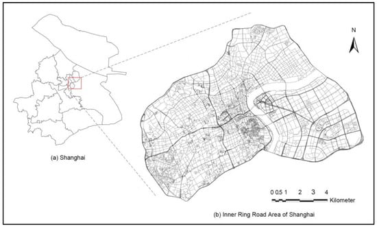
Figure 1.
Study area: areas within Shanghai’s Inner Ring Road.
3.2. Data Sources
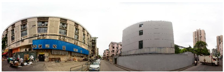
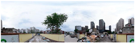
3.2.1. Baidu Street View Images
Baidu Map is an online map service provided by Baidu []. The panoramic static image service provided by Baidu Map (https://map.baidu.com, accessed on 31 January 2022) is similar to GSV. In this study, 8220 street panoramic images with the resolution of 1024 dpi × 512 dpi were downloaded based on the coordinates of dining spots within Shanghai’s Inner Ring Road, through the panoramic static image application programming interface provided by the Baidu map developer platform. This study uses the proportion of common street elements—plants, sky, and people’s views of sidewalks—as the independent variables, to explore the relationship between the elements and the rating data.
3.2.2. Dazhong Dianping Data
The review data of restaurant consumers were extract from the Dazhong Dianping website. Dazhong Dianping is the largest third-party consumer rating website in China and employs professional offline sales staff to check and update store information on the spot. As an authoritative and representative network, the website’s data provide a comprehensive overview of merchant information and consumer evaluations.
With the help of a web crawler, the study extracted the types, coordinates, cumulative number of reviews, consumers’ taste ratings, indoor environment ratings, service ratings, and consumption per capita of the 21,065 restaurants within Shanghai’s Inner Ring Road. The number of reviews, the three types of ratings, and the consumption per capita were chosen as the dependent variables to examine the relationship between them and the environment quality of the built spaces in the subsequent least square regression analysis.
3.3. Research Tools
3.3.1. Image Semantic Segmentation
Using image segmentation technology of deep learning and with the aid of Google Cityscapes’ urban dataset and the DeepLab-v3 deep learning model, this study segmented 19 elements in urban street view images, namely road, sidewalk, building, wall, fence, pole, traffic light, traffic sign, vegetation, terrain, sky, person, rider, car, truck, bus, train, motorcycle, and bicycle (Table 1), to quantify the composition of visible streets and obtain the category of each element in the street view map with relatively high accuracy. Images with segmented street elements already carry elements’ information, but still lack quantitative results. Therefore, Python 3.7.2 was used to calculate in batches the proportion of each element in the images after segmentation.

Table 1.
Segmentation items in the recognition of images in Google Cityscapes’ ratings dataset.
The abovementioned 16 elements were used in the analysis of this study. The proportion of walls and fences were taken as the interface encirclement, and the proportions of cars, trucks, and buses as the motor vehicle interference index. This left a total of 13 independent variables in the built environment category (Table 2).
Table 2.
Independent variables.
3.3.2. People’s Willingness to Stay
BSV objectively evaluates street quality from the perspective of a physical space, while people’s willingness to stay subjectively evaluates street quality from the perspective of people’s perceptions of a physical space. Willingness to stay is taken as one of the independent variables of this study, along with road network density, road walkability, green view rate, and sky openness. The quantification of people’s willingness to stay can be used to evaluate people’s intuitive perception of space quality and increase the dimensions of the discussion on space quality of a built environment.
Drawing on widely accepted evaluation criteria in the existing literature [] based on the imaginative character, human scale and transparency, tidiness, vegetation coverage and people’s psychological feelings, sample images corresponding to the ratings of 1 to 5 were selected for reference. Deep learning was used to rate the pedestrians’ willingness to stay on a scale of 1 to 5 (Table 3).
Table 3.
Examples of the rating criteria for people’s willingness to stay corresponding to the quality of the street space.
3.3.3. Environmental Quality Evaluation Model
After examining the extracted images, we selected 5% of the 8220 images for the sample (420 street panoramas, of which 70% were used for training, 20% for tests, and 10% for validation), and invited three designers who had received systematic education in urban and rural planning to rate the images.
Next, we trained several state-of-the-art CNN models, such as DenseNet-121 [], SENet-154 [], ResNeSt-50d [] and Inception-v4 [], and compared the accuracy verification results of four CNN-based classification models (Figure 2). Lastly, the Inception-v4 model was selected. The propensity score matching of willingness to stay in the remaining 95% of the samples (7820 street panoramas) was carried out using the Inception-v4 deep learning model. When predicting the 1 to 5 ratings of willingness to stay, the accuracy of the Inception-v4 model reached 62%, 65%, 74%, 53% and 79%, respectively.
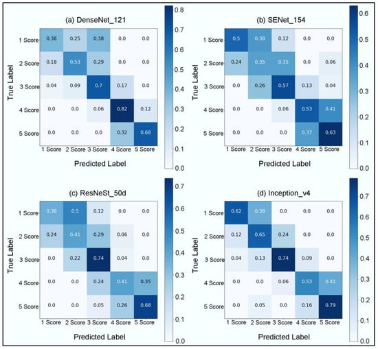
Figure 2.
The test images of the normalized confusion matrices of correlations that evaluated the four networks.
3.3.4. Eliminating the Outliers
Based on the 3σ principle in a normal distribution, the probability that the values are distributed in (μ − 3σ, μ + 3σ) is 0.9974, the probability that the variables fall outside (μ − 3σ, μ + 3σ) is less than three thousandths, and it is assumed that the corresponding event will not occur in practical problems. Therefore, in order to increase the reliability of the experimental results, the data of each item falling outside three standard deviations were eliminated. This left final sample of 16,794 items of data.
3.3.5. The Least Squares Method
The study used a least square regression analysis to explore further the spatial correlation between the independent variables and the dependent variable, namely the space quality of the built environment. The least squares method finds the optimal function matching of the data by minimizing the sum of squared residuals, which is a commonly used statistical method for reconstructing phylogenetic trees []. The unknown data can be easily obtained by using the least squares method, and the sum of squared residuals between the obtained data and the actual data can be minimized. In this study, it can be used to determine the quantitative relationship between elements in the outdoor built environment near the dining spots and consumer preferences.
The basic principle is as follows:
Let (x, y) be a pair of observations that satisfy in the following theoretical function:
in which is the parameter to be determined.
To find the optimal estimate of parameter in function , for the given m sets (usually ) of observed data , the objective function
takes the minimum value of the parameter . The type of problem to be solved is called a least squares problem, and the geometric language for solving this problem is called a least squares fitting.
For unconstrained optimization problems, the general form of the least squares method is
where is called the residual function. When is the linear function of x, it is called a linear least squares problem, otherwise it is called a nonlinear least squares problem.
3.4. Research Framework
Taking dining spots as the examples, this study (1) used the BSV panoramas within Shanghai’s Inner Ring Road and quantified the composition of visible streets with semantic segmentation. (2) A selection was performed using confusion matrices of willingness to stay, and an Inception-v4 model was chosen to perform an inference of a 1–5 scale on 8220 street panoramas. (3) Data from the Dazhong Dianping website was extracted using a crawler program to obtain people’s ratings on their dining experience in the restaurants; ArcGIS 10.6 was used to visualize the types, number of reviews, consumers’ taste ratings, indoor environment ratings, service ratings, and consumption per capita of the 21,065 restaurants within Shanghai’s Inner Ring Road. (4) Based on the 3σ principle in mathematical statistics, data that fell outside three standard deviations were eliminated to obtain a final selection of 16,794 data items. (5) Based on the coordinates, a least squares regression analysis was performed on the environment quality of the physical spaces, people’s willingness to stay, and the popularity of the place. Lastly, the relationship between physical environment features around the restaurants, the ratings of people’s willingness to stay and the people’s preferences, were quantified to provide references for optimizing land use, enhancing the livability of megacities, and ensuring high-quality urban development. The analytical framework is summarized in Figure 3.
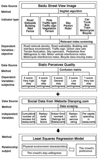
Figure 3.
Indicator system and analytical framework.
4. Results
4.1. Space Quality Analysis
4.1.1. Physical Environment Analysis
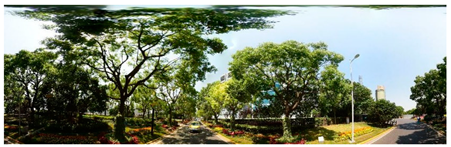
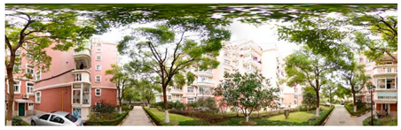
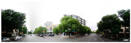
As shown in Figure 4, this study used the image segmentation technology of deep learning to classify panoramic BSV images into 19 items, including roads, sidewalks and buildings, in a statistical summary table.
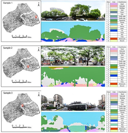
Figure 4.
Segmentation demos by Deeplab.
The images in the segmentation results were imported to the ArcGIS 10.6 platform for the classification of unique values. Pixels with different content are labeled with different colors to make them distinguishable (Figure 5). The counts of the pixels corresponding to the different content could be obtained by examining the attributes table and were used as independent variables in the subsequent regression analysis.
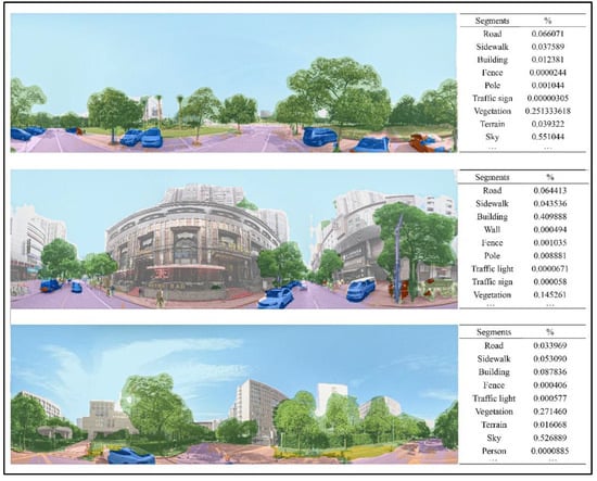
Figure 5.
Summary table of the segmentation results.
4.1.2. Analysis of Stay Willingness
The number of images with a total score of 4 (6907) and 5 (5558) accounted for 59.17% of the total number of images; the number of images with a score of 3 (4724) accounted for 22.43% of the total, the number of images with a total score of 1 (531) and 2 (3345) accounted for 18.40% of the total. The results indicate that pedestrians’ willingness to stay in the areas surrounding more than half of the restaurants within Shanghai’s Inner Ring Road is relatively high, and more than 80% of the restaurants can expect pedestrians to linger in the area. The results are illustrated in Figure 6.
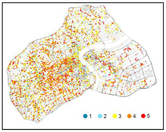
Figure 6.
Rating results of willingness to stay.
4.2. Restaurant Evaluation Results
The visualization of the data on the ArcGIS 10.6 platform shows that 91.13% (n = 19,197) of the restaurants received 1–3390 reviews. The restaurants with a high number of reviews, which were extremely rare, are generally clustered in Huaihai Road and West Beijing Road. The results show that 51.29% of the restaurants received taste ratings below 7.6 (10,805), while nearly half of the restaurants, scattered throughout the study area, received ratings above 7.6. In addition, 42.61% of restaurants with an indoor environment received ratings below 7.4 (8976), and more than half of restaurants, scattered throughout the study area, received ratings above 7.4. A total of 43.96% of the restaurants received service ratings below 7.4 (9261), and more than half of the restaurants with a rating above 7.4 and were scattered in the study area. Lastly, 58.90% of restaurants reported a consumption per capita of 63 RMB or less (12,407), and 84.59% reported a consumption per capita of 142 RMB or less (17,819). In addition, no more than one-fifth of the high-consumption restaurants showed a trend of “large dispersion and small clustering,” with a certain degree of clustering on the east and west sides of the Huangpu River and the intersection of Caoyang Road and Huashan Road. The results are illustrated in Figure 7.
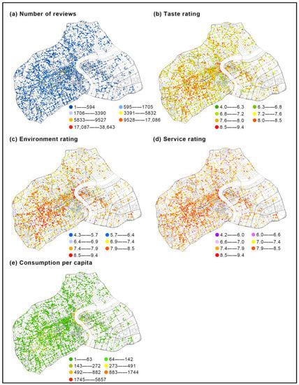
Figure 7.
Spatial distribution of the social media data.
4.3. Analysis Results of the Least Squares Method
4.3.1. Pearson’s Correlation Analysis
We imported the data into the IBM SPSS Statistics 26 platform and conducted a Pearson’s correlation analysis. The analysis found that most variables show a significant correlation at the 0.01 level, and a few variables, such as consumption per capita and terrain fluctuation, have a significant correlation at the 0.05 level. There are also variables that do not have a significant correlation at the 0.05 level, such as taste rating and building rate. The results are summarized in Table 4 and illustrated in Figure 8.
Table 4.
Pearson’s correlation analysis results.
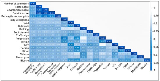
Figure 8.
Results of the Pearson’s correlation.
4.3.2. Results of the Spatial Autocorrelation Analysis
The spatial autocorrelation analysis shows that when the dependent variables are the number of reviews, taste rating, indoor environment rating, service rating, and consumption per capita, the z-scores are higher; therefore, the probability that this clustering pattern is randomly generated is less than 1%. The results are illustrated in Figure 9. In order to further explore the functional relationship between the space quality of the built environment and the restaurant review data, we conducted a least squares analysis in the following section.
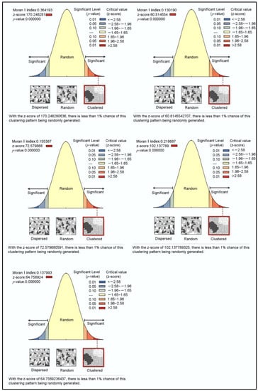
Figure 9.
Results of the spatial autocorrelation analysis results (upper row, from left to right: the dependent variables, namely the number of reviews and sum of taste ratings; middle row, from left to right: the dependent variables, namely indoor environment rating and service rating; and bottom row, the dependent variable, consumption per capita).
4.4. Least Squares Analysis
Taking the number of restaurant reviews as the dependent variable, an ordinary least squares (OLS) analysis shows that the independent variables that are significant at the 0.01 level included traffic sign, person, and bicycle, and the independent variable that is significant at the 0.05 level was terrain. Therefore, (1) the built environment elements with the greatest effect on the number of restaurant reviews include density of traffic signs, pedestrian flow, bicycle slow-moving index, and terrain fluctuation. Among them, density of traffic signs has a significant negative effect on the number of reviews, while pedestrian flow has a significant positive effect on the number of reviews, exceeding the other two elements. (2) The lower the density of traffic signs in an area, the higher the number of reviews. (3) The higher the pedestrian flow in an area, the higher the number of reviews. (4) The higher the bicycle slow-moving index in an area, the higher the number of reviews. Lastly, (5) there is a significant positive correlation between terrain fluctuation and the number of reviews. The results are summarized in Table 5.
Table 5.
OLS analysis with number of reviews as the dependent variable (n = 16,794).
Taking the taste rating of restaurants as the dependent variable, an OLS analysis shows that the relevant independent variables with significance at the 0.01 level include road, sidewalk, building, vegetation, terrain, sky, person, vehicle, and bicycle, while encirclement is significant at the 0.05 level. All the dependent variables show a significant positive correlation with the number of reviews. Therefore, (1) the built environment elements with the greatest effect on the taste rating of restaurants include pedestrian flow, bicycle slow-moving index, terrain fluctuation, road walkability, motor vehicle interference index, green view rate, building rate, sky openness, road network density, and interface encirclement, while pedestrian flow has the greatest effect, followed by bicycle slow-moving index. The other factors did not make a significant difference in the degree of effect. Additional findings are: (2) the higher the pedestrian flow, the higher the taste rating; (3) the higher the bicycle slow-moving index and the more developed the non-motorized traffic in an area, the higher the taste rating of restaurants; and (4) the higher the terrain fluctuation of an area, the higher the taste rating; (5) the higher the greening rate and the sky openness of a street, the higher the ratings of consumers. (6) Building rate and interface encirclement also positively promoted the taste ratings of a restaurant. (7) An increase in the motor vehicle interference degree and road network density also contributed to an increase in taste ratings. The results are summarized in Table 6.
Table 6.
OLS analysis with taste rating as the dependent variable (n = 16,794).
Taking the indoor environment rating of restaurants as the dependent variable, an OLS analysis shows that the independent variables with significance at the 0.01 level include sidewalk, building, vegetation, terrain, sky, person, and vehicle, while the independent variables with significance at the 0.05 level include willingness to stay, road, and bicycle. Pedestrian flow has the greatest effect on ratings, while the effect of people’s willingness to stay is relatively weak and negative. All other factors have a positive effect and make little difference in the degree of effect. Therefore, (1) the built environment elements with the greatest effect on the indoor environment rating of restaurants include pedestrian flow, bicycle slow-moving index, road walkability, green view rate, building rate, terrain fluctuation, sky openness, road network density, motor vehicle interference index, and people’s willingness to stay. The results also show that (2) the higher the pedestrian flow around a restaurant, the higher the indoor environment rating; (3) the higher the bicycle slow-moving index and the higher the road walkability in an area, the higher the indoor environment rating of the restaurant; and (4) the higher the green view rate, the greater the sky openness, and the greater the terrain fluctuation of a street, the higher the restaurant’s ratings. (5) Building rate promotes the indoor environment rating of a restaurant. (6) Areas with high road network densities and motor vehicle interference indices receive higher ratings for dining atmosphere. (7) There is also a significant negative correlation between willingness to stay and the indoor environment rating. The results are summarized in Table 7.
Table 7.
OLS analysis with indoor environment rating as the dependent variable (n = 16,794).
Taking the service rating of restaurants as the dependent variable, an OLS analysis, shows that the independent variables with significance at the 0.01 level include road, sidewalk, building, vegetation, terrain, sky, person, vehicle, and bicycle, while willingness to stay is the independent variable with significance at the 0.05 level. Pedestrian flow has the greatest effect on environment ratings. Therefore, (1) the built environment elements that have the greatest effect on the service ratings of restaurants include pedestrian flow, road walkability, bicycle slow-moving index, green view rate, building rate, motor vehicle interference index, sky openness, terrain fluctuation, road network density, and people’s willingness to stay. The results also show that (2) the higher the pedestrian flow around the restaurant, the better the service; (3) the higher the road walkability and the higher the bicycle slow-moving index of an area, the higher the service ratings; (4) the higher the green view rate and the greater the sky openness and terrain fluctuation, the higher consumers rate the restaurants’ service quality. (5) Building rate also promotes the service rating of a restaurant. (6) In areas with high road network density and motor vehicle interference degree, restaurants provide high-quality services to win the support of consumers. (7) There is also a significant negative correlation between willingness to stay and service rating. The results are summarized in Table 8.
Table 8.
OLS analysis with service rating as the dependent variable (n = 16,794).
Taking the consumption per capita of restaurants as the dependent variable, an OLS analysis shows that the independent variables with a significant positive effect at the 0.01 level include traffic sign and person, while the independent variables with a significant positive effect at the 0.05 level include rider and bicycle. Therefore, (1) the built environment qualities with the greatest effect on consumption per capita include density of traffic signs, pedestrian flow, and bicycle slow-moving index, among which the density of traffic signs is the most significant, while the number of riders has a significant negative effect on consumption per capita. (2) In this study, the higher the density of traffic signs in an area, the higher the consumption per capita; (3) the higher the pedestrian flow in an area, the higher the consumption per capita; (4) the higher the bicycle slow-moving index in an area, the higher the consumption per capita; and (5) the more riders in an area, the lower the consumption per capita. The results are summarized in Table 9.
Table 9.
OLS analysis with consumption per capita as the dependent variable (n = 16,794).
5. Discussion
This study shifts from the two-dimensional perspective of remote sensing images to a three-dimensional perspective of street view imagery to examine the quality of physical spaces and people’s subjective evaluations of public spaces. The study constructs a data-driven framework based on two major geographic data sources—street panoramic images and social media rating data—and uses semantic segmentation to quantify the visible components of streets. It adopts deep learning methods to construct a CNN-based classification model that adapts to the rating criteria of willingness to stay, to examine the relationship between the attributes of street spaces and ratings data on consumer websites.
Although earlier studies have conducted research by combining the use of street view images and social media data [,], their understanding of the types of social media data is relatively narrow and therefore limited to point-of-view (POI) data extracted from platforms such as Weibo and Twitter. To the best of our knowledge, our study is the first to examine the quality of the built environment, while, at the same time, extending the scope of social media data to include data from post-use rating websites. Comment data has a large amount of dissemination and a strong cumulative effect, which can reflect the preferences of both the resident population and the floating population, overcoming the severe time lag of traditional research data. The study of the relationship between the quality of the built environment and the popularity of restaurants is an example of a real-life application of the study, in which the screening of factors that have a significant impact on consumer evaluation is useful for restaurants to improve their operational efficiency as much as possible, even if this is not the only way to improve efficiency, but it is useful for operators to improve a little efficiency and evaluation results in the current competitive market. Reducing the proportion of projects in the built environment that inhibit the popularity of restaurants, and increasing the proportion of projects that promote the popularity of restaurants may help to improve the economic vitality of Chinese cities [], especially in an era when China’s economic growth mainly depends on the growth of service industry in urban areas. Taking crowd perception data and built environment semantic segmentation data together as independent variables can make up for the shortcomings of previous research and form a closed loop that starts from human perception and then returns to human perception.
We only select common elements in streetscape images that characterize the built environment from the perspective of the built environment and investigate whether and to what extent they have an impact on the popularity of the restaurant. The current experiment can only prove that when a certain element of the built environment is changed, there is a certain change in the evaluation results; that is, there is a correlation between them, but we cannot prove that there is an obvious causal relationship between them, because the change in the environment may affect other factors that we have not yet explored (such as wages, people living around, consumption levels, etc.), and then these factors affect the evaluation results, so the study does have limitations.
With the help of social media data obtained from the web, this study intuitively reflects the spatial distribution characteristics of consumers’ preferences for restaurants, and further explores the space quality factors that affect the popularity of dining places. The results show that traffic signs are a variable that is significantly negatively correlated with the number of reviews. This is because most of the older dining spots are located in the deep alleys of old streets in which people can only walk and where there are very few traffic signs for motor vehicles. Pedestrian flow is the variable with the greatest effect on taste, indoor environment, and service ratings. That is because pedestrian flow is related to the pedestrian friendliness of a street: the more popular the area among pedestrians, the greater the flow of people, and the higher the exposure of restaurants, so the probability of people dining in them is higher. Space quality factors include (1) natural factors, such as green view rate, terrain fluctuation, and sky openness, (2) traffic influencing factors such as road network density and motor vehicle interference index, and (3) artificial environment factors such as building rate, these all contribute to higher quality scores. However, the intensity of the effect is far less than pedestrian flow or the two independent variables that reflect the pedestrian friendliness of streets.
There is also a significant negative correlation between people’s willingness to stay and ratings. Common sense dictates that the area within Shanghai’s Inner Ring Road has many street food vendors. The operators of so-called “greasy spoons”, which are favored by low-income groups, are usually accessible and friendly, and the food is served with enthusiasm. Restaurants in areas with a higher density of traffic signs report higher levels of consumption per capita. Such areas are closer to the center of the region, and the restaurants have to raise prices to support normal operations under the pressure of higher rents. In addition, areas with a higher proportion of riders have lower levels of consumption per capita. A possible reason is that most of the people belong to the middle- and low-income groups, and they prefer to eat at small diners on the street that serve food at affordable prices.
This study used BSV images obtained and the coordinates of restaurants in Shanghai’s Inner Ring Road. However, due to the influence of image coverage and offset errors, the actual street images at the locations of the restaurant were not completely consistent with the obtained images. Second, the obtained BSV images lack a time dimension as a reference. In a small number of images, the buildings were either being renovated, or the roads were being repaired, so the elements captured from the decomposed images could only represent the state of the street at the time when the image is shot, and without long-term representation. Therefore, the image semantic segmentation results may be slightly different from the daily situation. Lastly, the panoramic static image downloaded through the Baidu API has a maximum resolution of 1024 dpi × 512 dpi, therefore the boundary information of objects was difficult to capture during the semantic recognition of the images. The blurred boundaries were often not clearly segmented, which interfered with the accuracy of the results of the pixel segmentation. In addition, the social media data collected came from the www.dianping.com (accessed on 31 January 2022). On the one hand, the source of the review data only represents the views of some groups. As some individuals have limited access to smartphones, some older adults and children’s perceptions of restaurants may have been excluded. On the other hand, there may be human errors in the ratings. For example, in extremely rare cases, restaurants may provide discounts or coupons to induce consumers to leave high ratings. These practices would undoubtedly interfere with the study’s experimental objectivity.
From remote sensing to street view images is a change in research perspective and from social media check-in data to consumers’ review data is an expansion of crowd coverage. Building a bridge between the visual elements and perception scores of street view images and consumer evaluations is an innovation in research direction. At the same time, the results inspire us to focus more on the innovation of research technology in future people-oriented planning, and to explore research methods that are better adapted to the human scale and meet consumers’ sensory expectations. In the future, the further utilization of professional pre-trained deep learning models will further improve research in this area. The diversified development of image acquisition equipment will also reduce difficulties related to image acquisition and improve image resolution, producing more accurate street view segmentation results.
In this study, street view images were acquired through the Baidu API, while on other platforms such as Tencent Maps, and historical image information, could also be downloaded. This may solve the problem of contingency in experiments and may even expand the research dimension. These are the directions for future research.
6. Conclusions
Taking restaurants as examples, we used state-of-the-art deep learning methods to process BSV panoramas. After eliminating outliers, the relationship between the environmental attributes of 16,794 dining spots within Shanghai’s Inner Ring Road and consumer review data were explored. OLS analyses used the number of reviews, taste rating, indoor environment rating, service rating and consumption per capita as the dependent variables. The space quality factors of the outdoor environment that became prominent under the effect of the different variables were discovered.
The following conclusions could be drawn. (1) The built environment qualities that affect the number of restaurant reviews include the density of traffic signs, pedestrian flow, bicycle slow-moving index, and terrain fluctuation; density of traffic signs has a significant negative effect on the number of reviews. (2) The most critical factor that affects the ratings on the taste of restaurant food, indoor environment, and service is pedestrian flow, followed by road walkability and bicycle slow-moving index, followed by natural factors (sky openness, greening rate, terrain fluctuation), traffic factors (road network density, motor vehicle interference index), and artificial environment factors (such as building rate), while people’s willingness to stay has a significant negative effect on the ratings. (3) The built environment qualities that affect consumption per capita include the density of traffic signs, street pedestrian flow and the degree of non-motorized design; the effect of density of traffic signs is the most significant.
This study is an urban scale-built environment evaluation empowered by new data and technologies. Unlike previous studies that focused on the impact of outdoor public green spaces on environmental quality and crowd perception, this paper unearths more factors that have an impact on the evaluation data after crowd use. Unlike traditional perceptions, we found that the density of traffic signs, pedestrian flow, and bicycle slow-moving index had more significant effects on the dependent variables than sky openness and green view rate.
In future work, we will continue to analyze in detail the influential roles between different elements and the influencing factors that play a decisive role in hotel evaluation, and further analyze the causal relationship between built environment quality and evaluation results. In terms of the trustworthiness of social media data, as “big data is not always better data” [], manual validation is also impractical due to the large datasets. Pablo Martí et al. propose a method for LBSN data retrieval, selection, classification and analysis [], which will help us in future research to improve the accuracy of social media data.
Author Contributions
Conceptualization, Yiwen Tang and Jiaxin Zhang; Data curation, Jiaxin Zhang; Formal analysis, Runjiao Liu; Funding acquisition, Runjiao Liu; Investigation, Yiwen Tang and Runjiao Liu; Methodology, Yiwen Tang and Jiaxin Zhang; Project administration, Runjiao Liu; Resources, Jiaxin Zhang; Software, Yiwen Tang, Jiaxin Zhang and Runjiao Liu; Supervision, Jiaxin Zhang and Yunqin Li; Validation, Jiaxin Zhang; Visualization, Yiwen Tang and Yunqin Li; Writing—original draft, Yiwen Tang; Writing—review and editing, Yunqin Li. All authors have read and agreed to the published version of the manuscript.
Funding
This research was funded by National Nature Science Foundation of China, grant number 52008397.
Institutional Review Board Statement
Not applicable.
Informed Consent Statement
Not applicable.
Data Availability Statement
Not applicable.
Conflicts of Interest
The authors declare no conflict of interest.
References
- Chen, M.; Gong, Y.; Lu, D.; Ye, C. Build a people-oriented urbanization: China’s new-type urbanization dream and Anhui model. Land Use Policy 2019, 80, 1–9. [Google Scholar] [CrossRef]
- Ma, L.; Cheng, W.; Qi, J. Coordinated evaluation and development model of oasis urbanization from the perspective of new urbanization: A case study in Shandan County of Hexi Corridor, China. Sustain. Cities Soc. 2018, 39, 78–92. [Google Scholar] [CrossRef]
- Yao, S.M.; Zhang, P.Y.; Yu, C.; Li, G.Y.; Wang, C.X. The theory and practice of new urbanization in China. Sci. Geogr. Sin. 2014, 34, 641–647. [Google Scholar]
- Mehta, V. The Street: A Quintessential Social Public Space; Routledge: London, UK; New York, NY, USA, 2013; ISBN 978-0-415-52710-1. [Google Scholar]
- Von Schönfeld, K.C.; Bertolini, L. Urban streets: Epitomes of planning challenges and opportunities at the interface of public space and mobility. Cities 2017, 68, 48–55. [Google Scholar] [CrossRef] [Green Version]
- Li, Y.; Yabuki, N.; Fukuda, T. Exploring the association between street built environment and street vitality using deep learning methods. Sustain. Cities Soc. 2022, 79, 103656. [Google Scholar] [CrossRef]
- Xu, F.; Jin, A.; Chen, X.; Li, G. New Data, Integrated Methods and Multiple Applications: A Review of Urban Studies based on Street View Images. In Proceedings of the 2021 IEEE International Geoscience and Remote Sensing Symposium IGARSS, Brussels, Belgium, 11–16 July 2021; IEEE: Brussels, Belgium, 2021; pp. 6532–6535. [Google Scholar]
- Ye, C.; Zhang, F.; Mu, L.; Gao, Y.; Liu, Y. Urban function recognition by integrating social media and street-level imagery. Environ. Plan. B Urban. Anal. City Sci. 2021, 48, 1430–1444. [Google Scholar] [CrossRef]
- Zhang, F.; Zu, J.; Hu, M.; Zhu, D.; Kang, Y.; Gao, S.; Zhang, Y.; Huang, Z. Uncovering inconspicuous places using social media check-ins and street view images. Comput. Environ. Urban. Syst. 2020, 81, 101478. [Google Scholar] [CrossRef]
- Cao, R.; Zhu, J.; Tu, W.; Li, Q.; Cao, J.; Liu, B.; Zhang, Q.; Qiu, G. Integrating Aerial and Street View Images for Urban Land Use Classification. Remote Sens. 2018, 10, 1553. [Google Scholar] [CrossRef] [Green Version]
- Xue, J.; Su, B. Significant Remote Sensing Vegetation Indices: A Review of Developments and Applications. J. Sens. 2017, 2017, 1–17. [Google Scholar] [CrossRef] [Green Version]
- Zhang, J.; Fukuda, T.; Yabuki, N. Development of a City-Scale Approach for Façade Color Measurement with Building Functional Classification Using Deep Learning and Street View Images. ISPRS Int. J. Geo-Inf. 2021, 10, 551. [Google Scholar] [CrossRef]
- Xiao, C.; Shi, Q.; Gu, C.-J. Assessing the Spatial Distribution Pattern of Street Greenery and Its Relationship with Socioeconomic Status and the Built Environment in Shanghai, China. Land 2021, 10, 871. [Google Scholar] [CrossRef]
- Guerrero-Prado, J.S.; Alfonso-Morales, W.; Caicedo-Bravo, E.F. A Data Analytics/Big Data Framework for Advanced Metering Infrastructure Data. Sensors 2021, 21, 5650. [Google Scholar] [CrossRef]
- Long, Y.; Liu, L. How green are the streets? An analysis for central areas of Chinese cities using Tencent Street View. PLoS ONE 2017, 12, e0171110. [Google Scholar] [CrossRef] [Green Version]
- Wu, D.; Gong, J.; Liang, J.; Sun, J.; Zhang, G. Analyzing the Influence of Urban Street Greening and Street Buildings on Summertime Air Pollution Based on Street View Image Data. Int. J. Geo-Inf. 2020, 9, 500. [Google Scholar] [CrossRef]
- Dong, R.; Zhang, Y.; Zhao, J. How Green Are the Streets within the Sixth Ring Road of Beijing? An Analysis Based on Tencent Street View Pictures and the Green View Index. Int. J. Environ. Res. Public Health 2018, 15, 1367. [Google Scholar] [CrossRef] [Green Version]
- Hu, A.; Zhang, J.; Kaga, H. Green View Index Analysis and Optimal Green View Index Path Based on Street View and Deep Learning. arXiv 2021, arXiv:2104.12627. [Google Scholar]
- Lu, Y. The Association of Urban Greenness and Walking Behavior: Using Google Street View and Deep Learning Techniques to Estimate Residents’ Exposure to Urban Greenness. Int. J. Environ. Res. Public Health 2018, 15, 1576. [Google Scholar] [CrossRef] [Green Version]
- Tao, Y.; Wang, Y.; Wang, X.; Tian, G.; Zhang, S. Measuring the Correlation between Human Activity Density and Streetscape Perceptions: An Analysis Based on Baidu Street View Images in Zhengzhou, China. Land 2022, 11, 400. [Google Scholar] [CrossRef]
- Zhang, L.; Ye, Y.; Zeng, W.; Chiaradia, A. A Systematic Measurement of Street Quality through Multi-Sourced Urban Data: A Human-Oriented Analysis. Int. J. Environ. Res. Public Health 2019, 16, 1782. [Google Scholar] [CrossRef] [Green Version]
- Hu, C.-B.; Zhang, F.; Gong, F.-Y.; Ratti, C.; Li, X. Classification and mapping of urban canyon geometry using Google Street View images and deep multitask learning. Build. Environ. 2020, 167, 106424. [Google Scholar] [CrossRef]
- Lin, T.; Lin, H.; Hu, M. Three-dimensional visibility analysis and visual quality computation for urban open spaces aided by Google SketchUp and WebGIS. Environ. Plan. B Urban Anal. City Sci. 2017, 44, 618–646. [Google Scholar] [CrossRef]
- Serra, M.; Hillier, B.; Karimi, K. Exploring countrywide spatial systems: Spatio-structural correlates at the regional and national scales. In Proceedings of the SSS 2015—10th International Space Syntax Symposium, London, UK, 13–17 July 2015. [Google Scholar]
- Appleyard, D.; Lintell, M. The Environmental Quality of City Streets: The Residents’ Viewpoint. J. Am. Inst. Plan. 1972, 38, 84–101. [Google Scholar] [CrossRef]
- Gehl, J.; Gemzøe, L. Public Spaces—Public Life; Arkitektens Forlag: Copenhagen, Denmark, 2004. [Google Scholar]
- Measuring Urban Design|SpringerLink. Available online: https://link.springer.com/book/10.5822/978-1-61091-209-9 (accessed on 28 March 2022).
- Dubey, A.; Naik, N.; Parikh, D.; Raskar, R.; Hidalgo, C.A. Deep Learning the City: Quantifying Urban Perception at a Global Scale. In Proceedings of the European Conference on Computer Vision, Glasgow, UK, 8–14 July 2016; Springer: Berlin/Heidelberg, Germany, 2016; pp. 196–212. [Google Scholar]
- Salesses, P.; Schechtner, K.; Hidalgo, C.A. The Collaborative Image of The City: Mapping the Inequality of Urban Perception. PLoS ONE 2013, 8, e68400. [Google Scholar] [CrossRef] [PubMed] [Green Version]
- Li, Y.; Yabuki, N.; Fukuda, T.; Zhang, J. A Big Data Evaluation of Urban Street Walkability Using Deep Learning and Environmental Sensors—A Case Study around Osaka University Suita Campus10; Osaka University: Osaka, Japan, 2020. [Google Scholar]
- Chai, Y.; Ta, N.; Ma, J. The socio-spatial dimension of behavior analysis: Frontiers and progress in Chinese behavioral geography. J. Geogr. Sci. 2016, 26, 1243–1260. [Google Scholar] [CrossRef]
- Qi, L.; Li, J.; Wang, Y.; Gao, X. Urban Observation: Integration of Remote Sensing and Social Media Data. IEEE J. Sel. Top. Appl. Earth Obs. Remote Sens. 2019, 12, 4252–4264. [Google Scholar] [CrossRef]
- Chen, Y.; Liu, X.; Gao, W.; Wang, R.Y.; Li, Y.; Tu, W. Emerging social media data on measuring urban park use. Urban For. Urban Green. 2018, 31, 130–141. [Google Scholar] [CrossRef]
- Chen, T.; Hui, E.C.M.; Wu, J.; Lang, W.; Li, X. Identifying urban spatial structure and urban vibrancy in highly dense cities using georeferenced social media data. Habitat Int. 2019, 89, 102005. [Google Scholar] [CrossRef]
- Naik, N.; Philipoom, J.; Raskar, R.; Hidalgo, C. Streetscore—Predicting the Perceived Safety of One Million Streetscapes. In Proceedings of the 2014 IEEE Conference on Computer Vision and Pattern Recognition Workshops, Long Beach, CA, USA, 23–28 June 2014; IEEE: Columbus, OH, USA, 2014; pp. 793–799. [Google Scholar]
- Ordonez, V.; Berg, T.L. Learning High-Level Judgments of Urban Perception. In Computer Vision—ECCV 2014; Lecture Notes in Computer Science; Fleet, D., Pajdla, T., Schiele, B., Tuytelaars, T., Eds.; Springer International Publishing: Cham, Switzerland, 2014; Volume 8694, pp. 494–510. ISBN 978-3-319-10598-7. [Google Scholar]
- Zhang, F.; Zhou, B.; Liu, L.; Liu, Y.; Fung, H.H.; Lin, H.; Ratti, C. Measuring human perceptions of a large-scale urban region using machine learning. Landsc. Urban Plan. 2018, 180, 148–160. [Google Scholar] [CrossRef]
- Fu, X.; Jia, T.; Zhang, X.; Li, S.; Zhang, Y. Do street-level scene perceptions affect housing prices in Chinese megacities? An analysis using open access datasets and deep learning. PLoS ONE 2019, 14, e0217505. [Google Scholar] [CrossRef]
- Helbich, M.; Yao, Y.; Liu, Y.; Zhang, J.; Liu, P.; Wang, R. Using deep learning to examine street view green and blue spaces and their associations with geriatric depression in Beijing, China. Environ. Int. 2019, 126, 107–117. [Google Scholar] [CrossRef]
- Biljecki, F.; Ito, K. Street view imagery in urban analytics and GIS: A review. Landsc. Urban Plan. 2021, 215, 104217. [Google Scholar] [CrossRef]
- Tang, J.; Long, Y. Measuring visual quality of street space and its temporal variation: Methodology and its application in the Hutong area in Beijing. Landsc. Urban Plan. 2019, 191, 103436. [Google Scholar] [CrossRef]
- Iandola, F.; Moskewicz, M.; Karayev, S.; Girshick, R.; Darrell, T.; Keutzer, K. DenseNet: Implementing Efficient ConvNet Descriptor Pyramids. arXiv 2014, arXiv:1404.1869. [Google Scholar]
- Hu, J.; Shen, L.; Albanie, S.; Sun, G.; Wu, E. Squeeze-and-Excitation Networks. IEEE Trans. Pattern Anal. Mach. Intell. 2020, 42, 2011–2023. [Google Scholar] [CrossRef] [PubMed] [Green Version]
- Zhang, H.; Wu, C.; Zhang, Z.; Zhu, Y.; Lin, H.; Zhang, Z.; Sun, Y.; He, T.; Mueller, J.; Manmatha, R.; et al. ResNeSt: Split-Attention Networks. arXiv 2020, arXiv:2004.08955. [Google Scholar]
- Szegedy, C.; Ioffe, S.; Vanhoucke, V.; Alemi, A.A. Inception-v4, Inception-ResNet and the Impact of Residual Connections on Learning. In Proceedings of the Thirty-First AAAI Conference on Artificial Intelligence, San Francisco, CA, USA, 4–9 February 2017. [Google Scholar]
- Rzhetsky, A.; Nei, M. Statistical properties of the ordinary least-squares, generalized least-squares, and minimum-evolution methods of phylogenetic inference. J. Mol. Evol 1992, 35, 367–375. [Google Scholar] [CrossRef]
- Ma, Y.; Yang, Y.; Jiao, H. Exploring the Impact of Urban Built Environment on Public Emotions Based on Social Media Data: A Case Study of Wuhan. Land 2021, 10, 986. [Google Scholar] [CrossRef]
- Wang, Y.; Gao, S.; Li, N.; Yu, S. Crowdsourcing the perceived urban built environment via social media: The case of underutilized land. Adv. Eng. Inform. 2021, 50, 101371. [Google Scholar] [CrossRef]
- Long, Y.; Huang, C. Does block size matter? The impact of urban design on economic vitality for Chinese cities. Environ. Plan. B Urban Anal. City Sci. 2019, 46, 406–422. [Google Scholar] [CrossRef] [Green Version]
- Ilieva, R.T.; McPhearson, T. Social-media data for urban sustainability. Nat. Sustain. 2018, 1, 553–565. [Google Scholar] [CrossRef]
- Martí, P.; Serrano-Estrada, L.; Nolasco-Cirugeda, A. Social Media data: Challenges, opportunities and limitations in urban studies. Comput. Environ. Urban Syst. 2019, 74, 161–174. [Google Scholar] [CrossRef]
Publisher’s Note: MDPI stays neutral with regard to jurisdictional claims in published maps and institutional affiliations. |
© 2022 by the authors. Licensee MDPI, Basel, Switzerland. This article is an open access article distributed under the terms and conditions of the Creative Commons Attribution (CC BY) license (https://creativecommons.org/licenses/by/4.0/).