
Developing Relative Spatial Poverty Index Using Integrated Remote Sensing and Geospatial Big Data Approach: A Case Study of East Java, Indonesia


Abstract
:1. Introduction
2. Materials and Methods
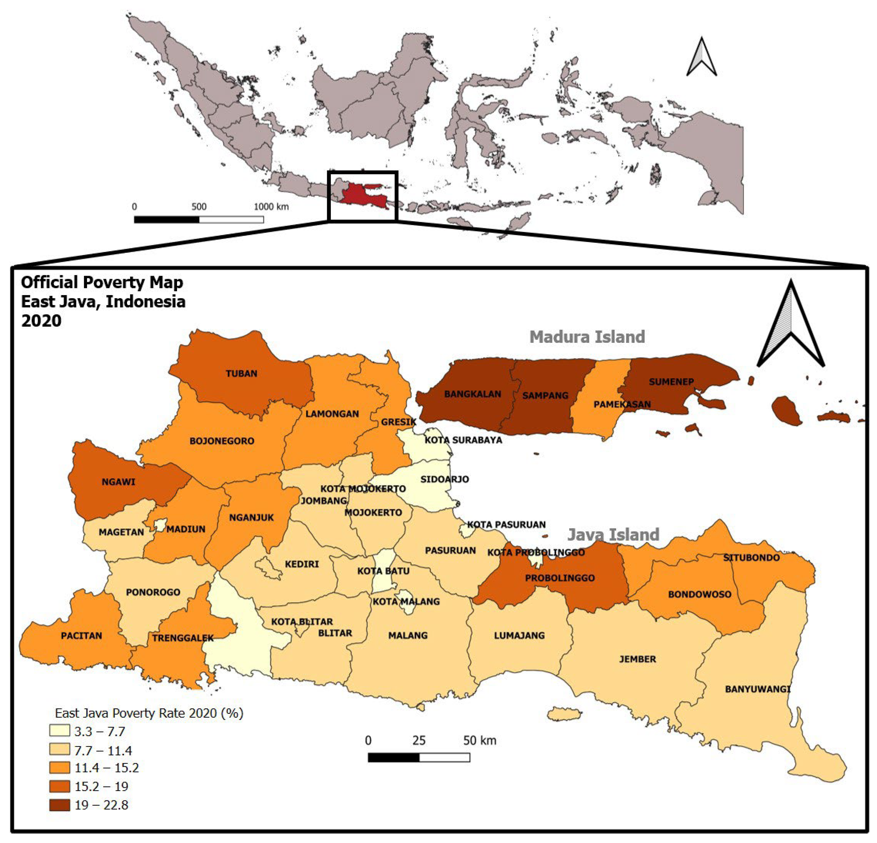
2.1. Study Area
2.2. Data Used in This Study
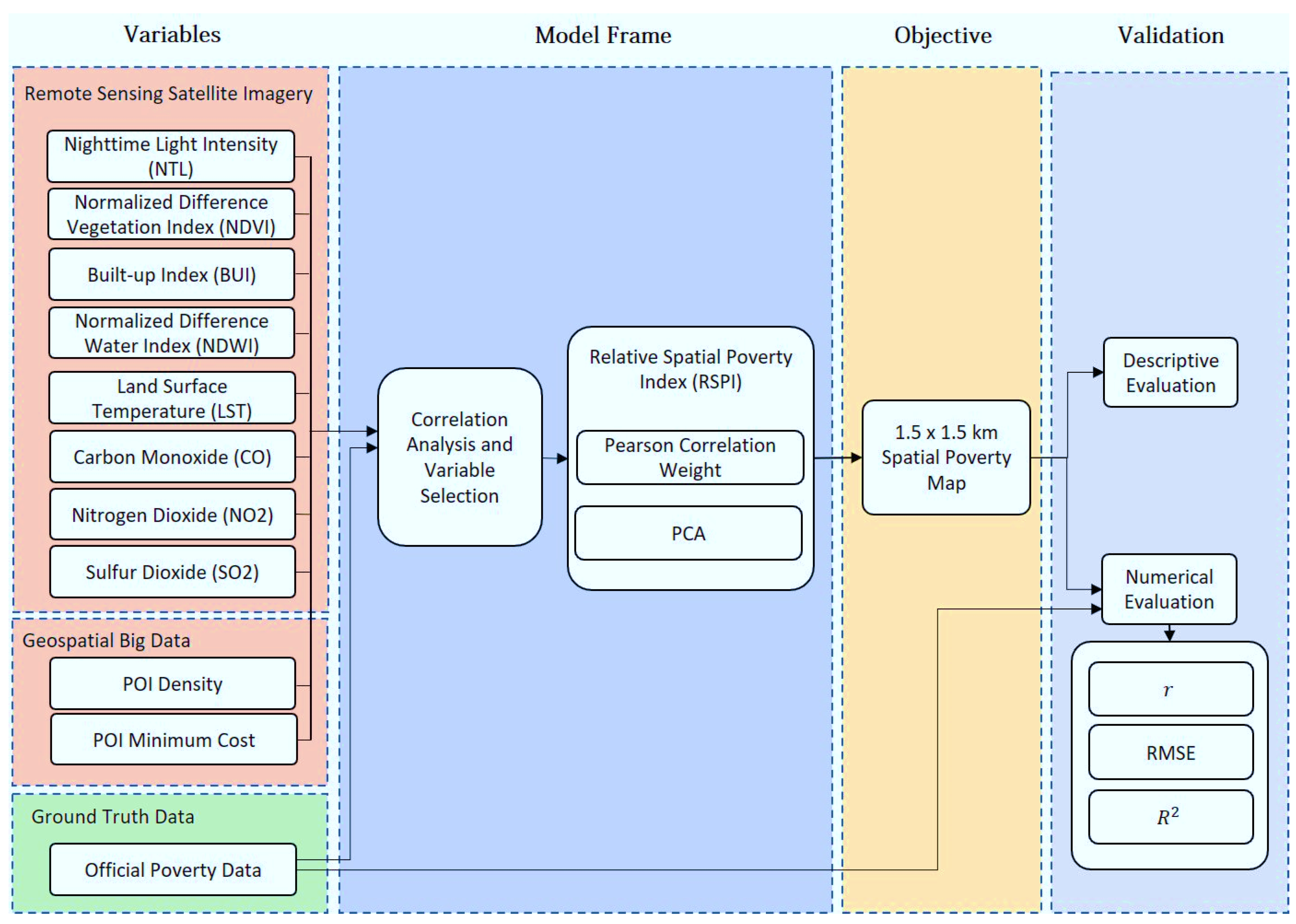
2.3. Methodology
2.3.1. Data Collection and Pre-Processing
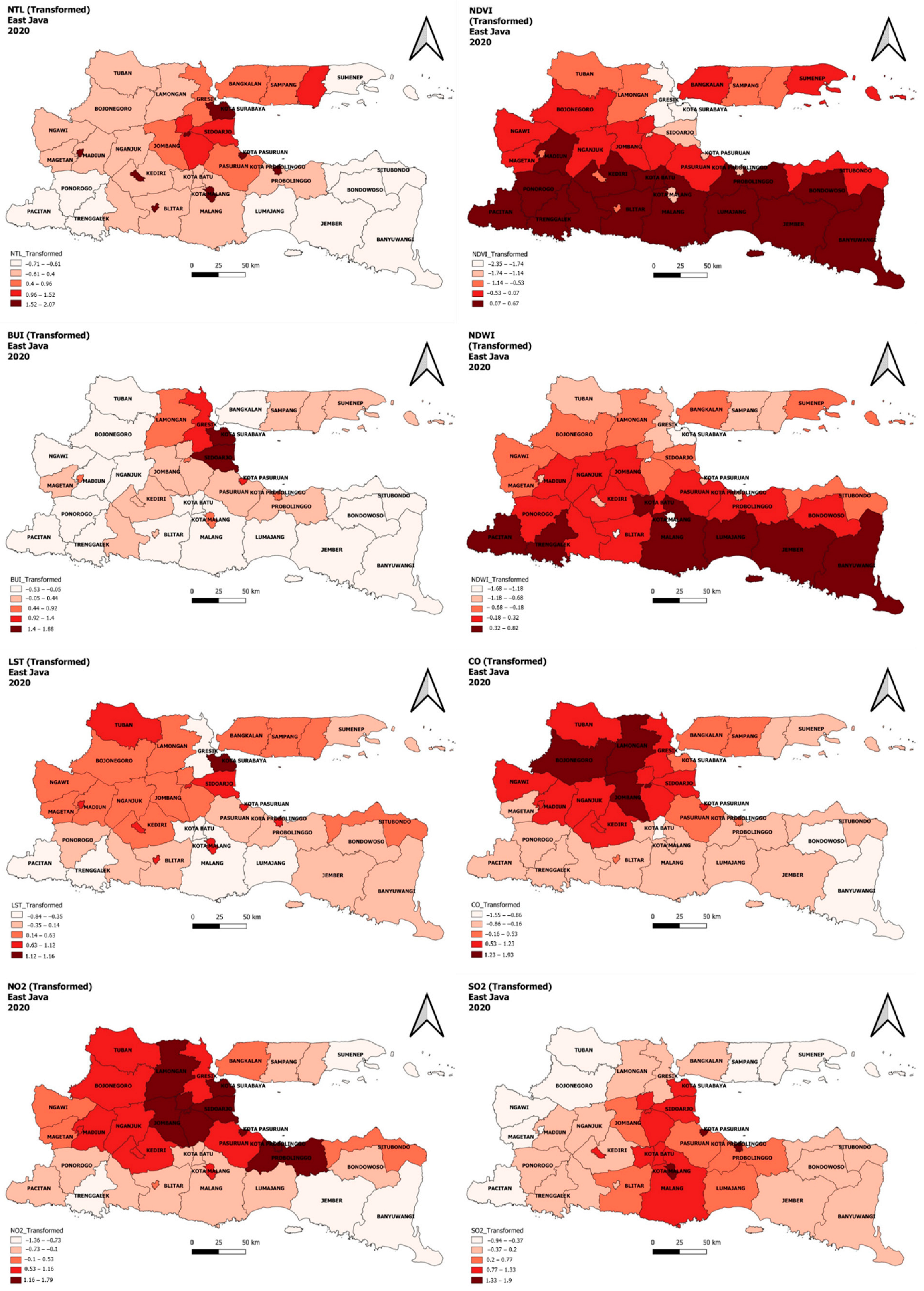
Remote Sensing Satellite Imagery Data Pre-Processing
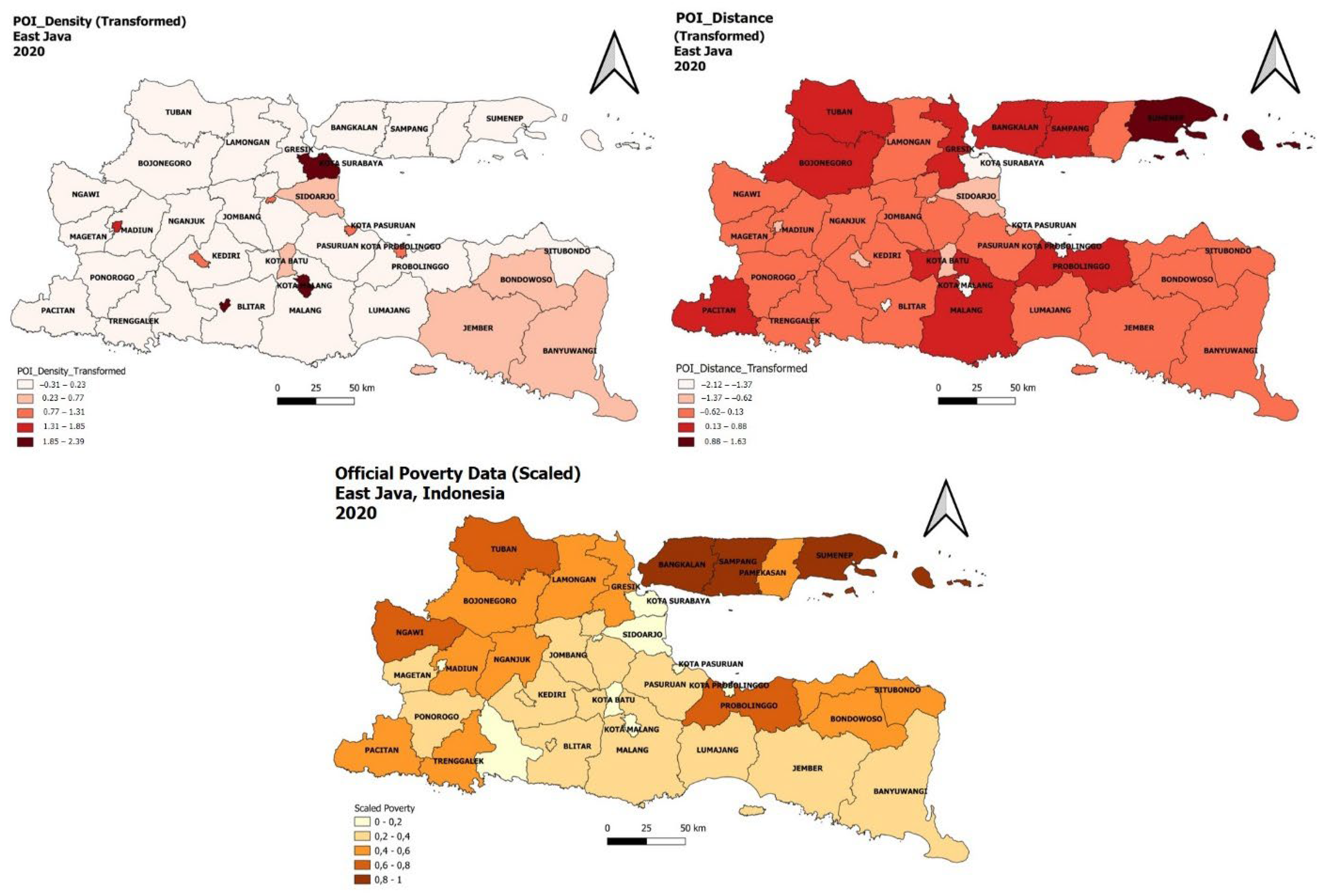
Geospatial Big Data Pre-Processing
2.3.2. Data Transformation
2.3.3. Data Integration
2.3.4. Correlation Analysis and Variable Selection
2.3.5. Relative Spatial Poverty Index (RSPI) Calculation
2.3.6. Validation Assessment
3. Results
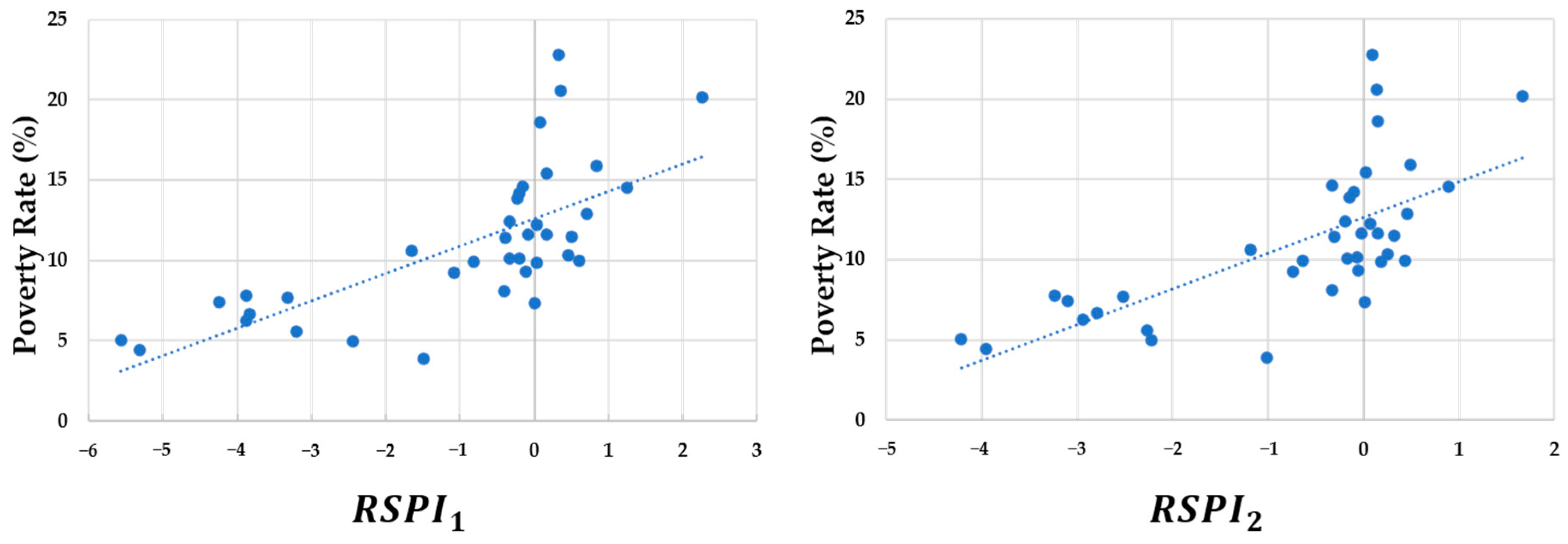
3.1. Correlation Model Development
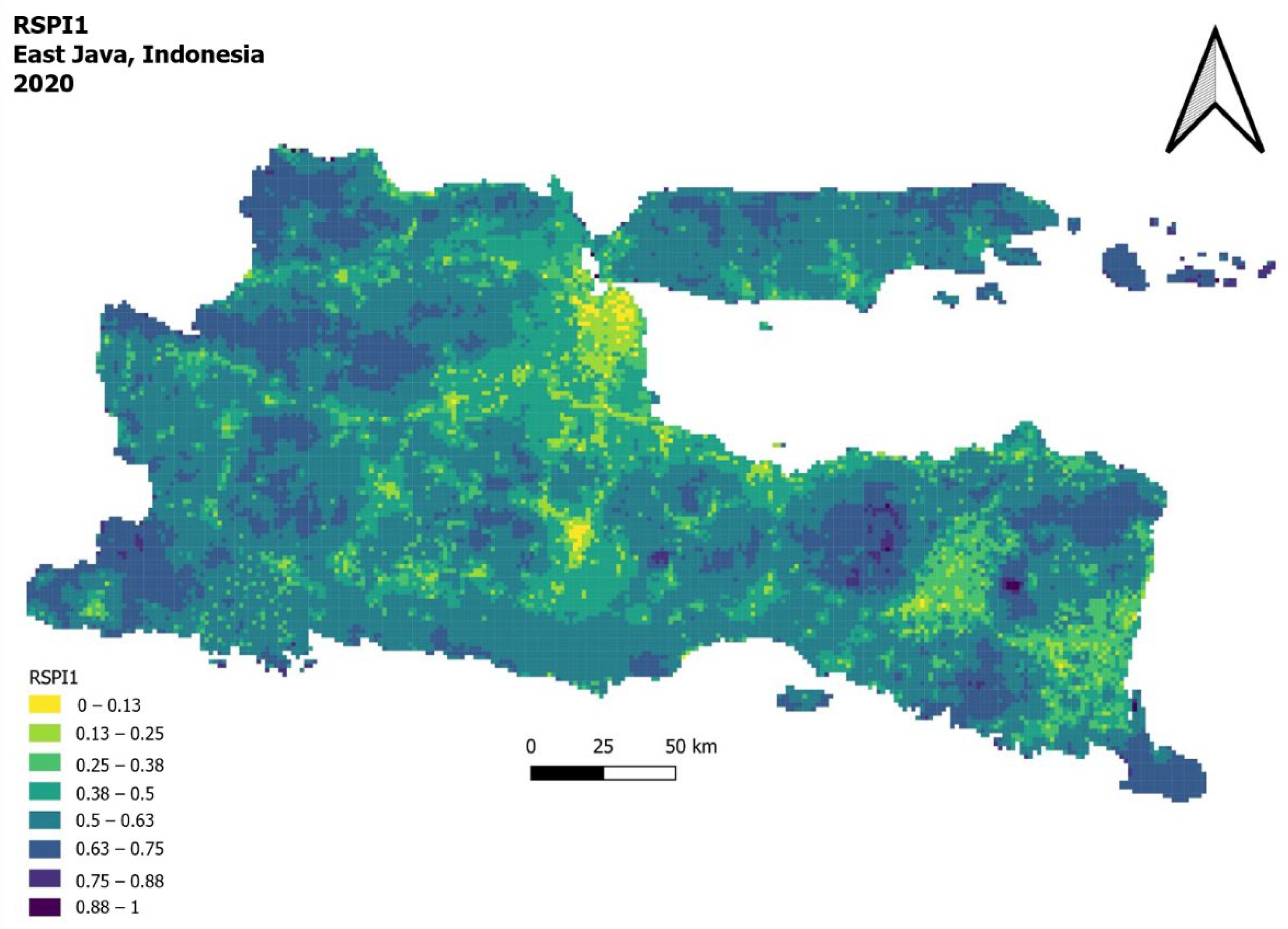
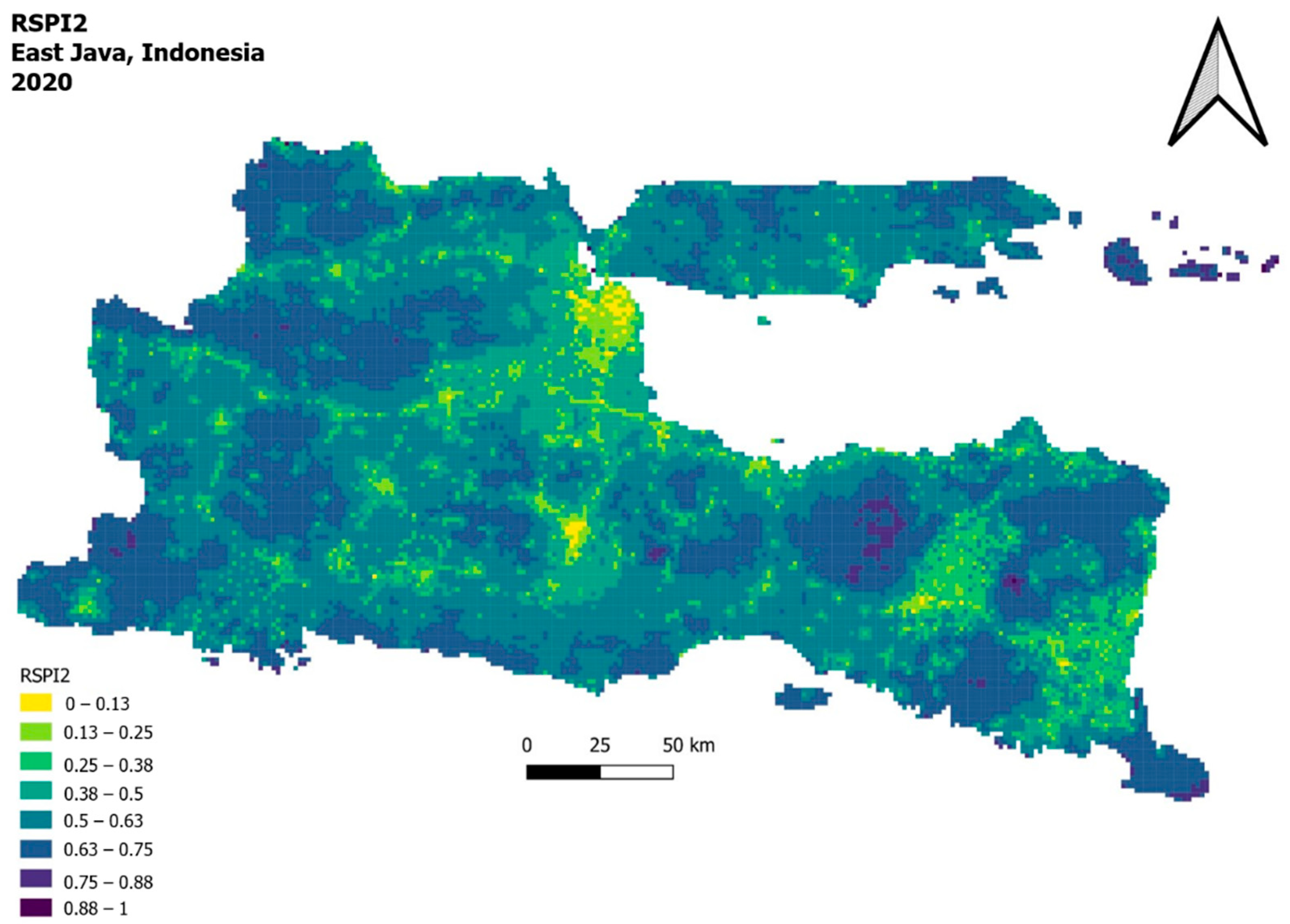
3.2. Relative Spatial Poverty Index Calculation
4. Discussion
4.1. RSPI Numerical Evaluation
4.2. RSPI Ground Truth Analysis
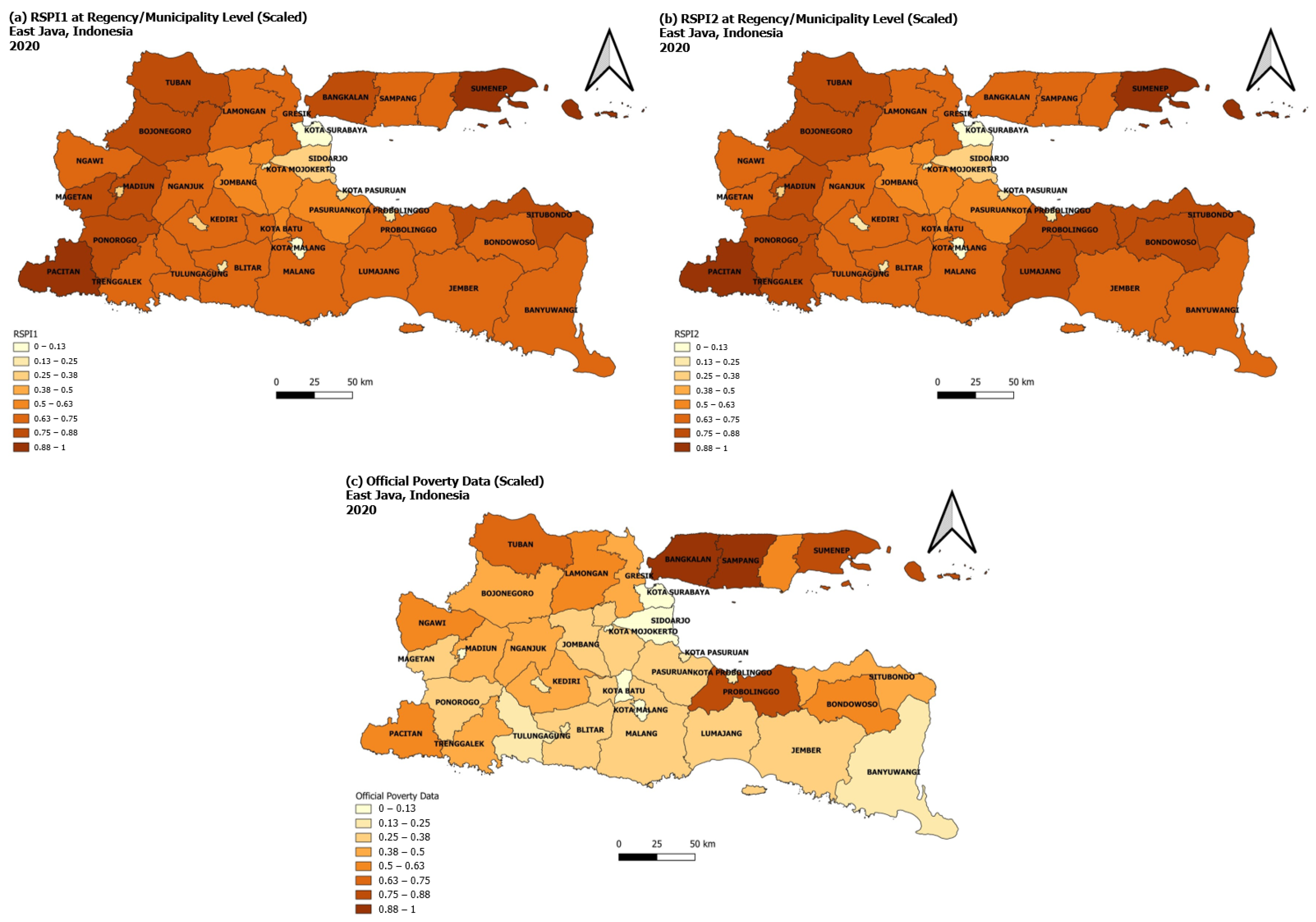
4.3. Comparison between the Obtained RSPI and the Official Poverty Data
4.4. Limitations and Future Possible Directions
5. Conclusions
Author Contributions
Funding
Informed Consent Statement
Data Availability Statement
Acknowledgments
Conflicts of Interest
Appendix A
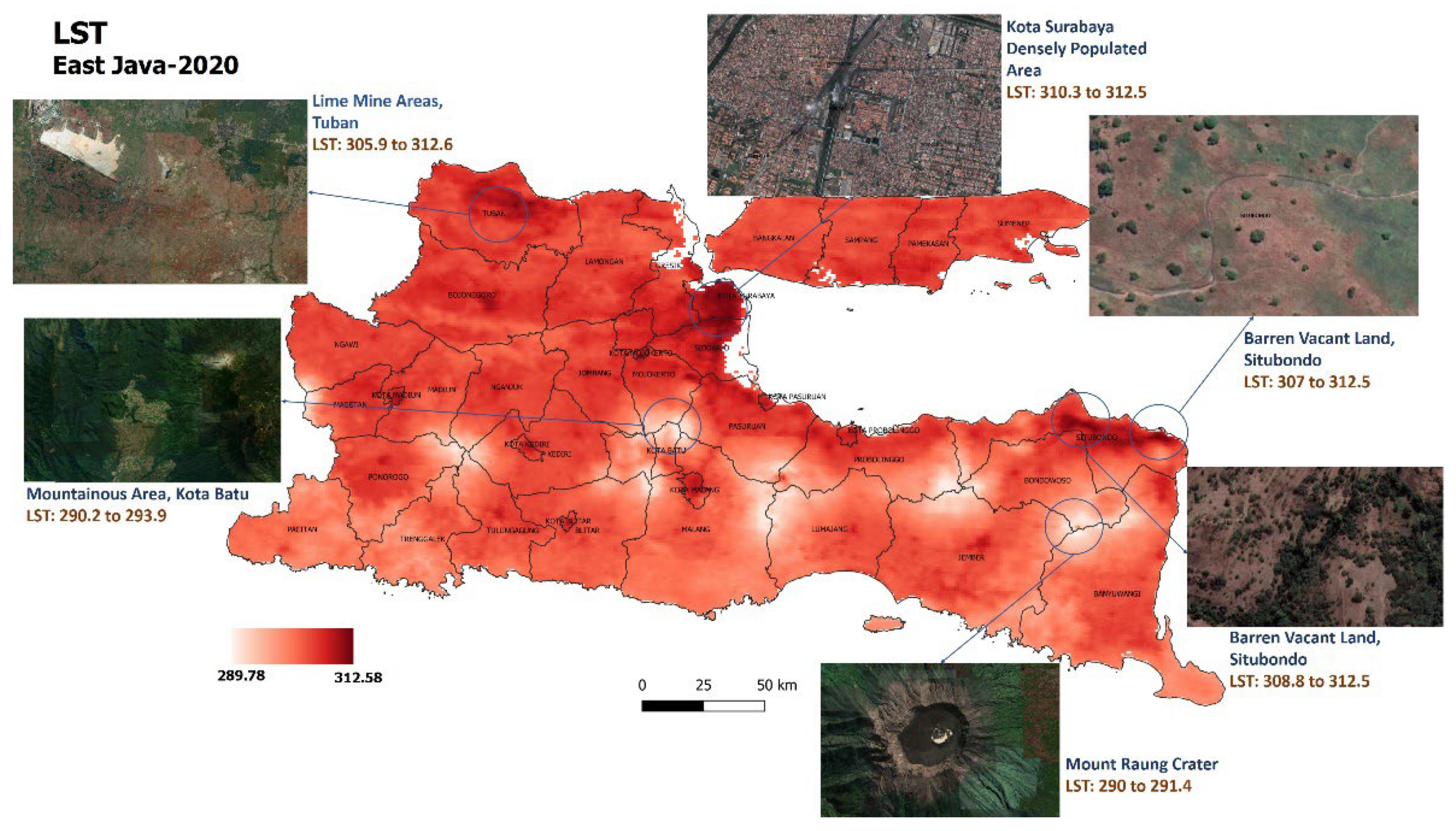
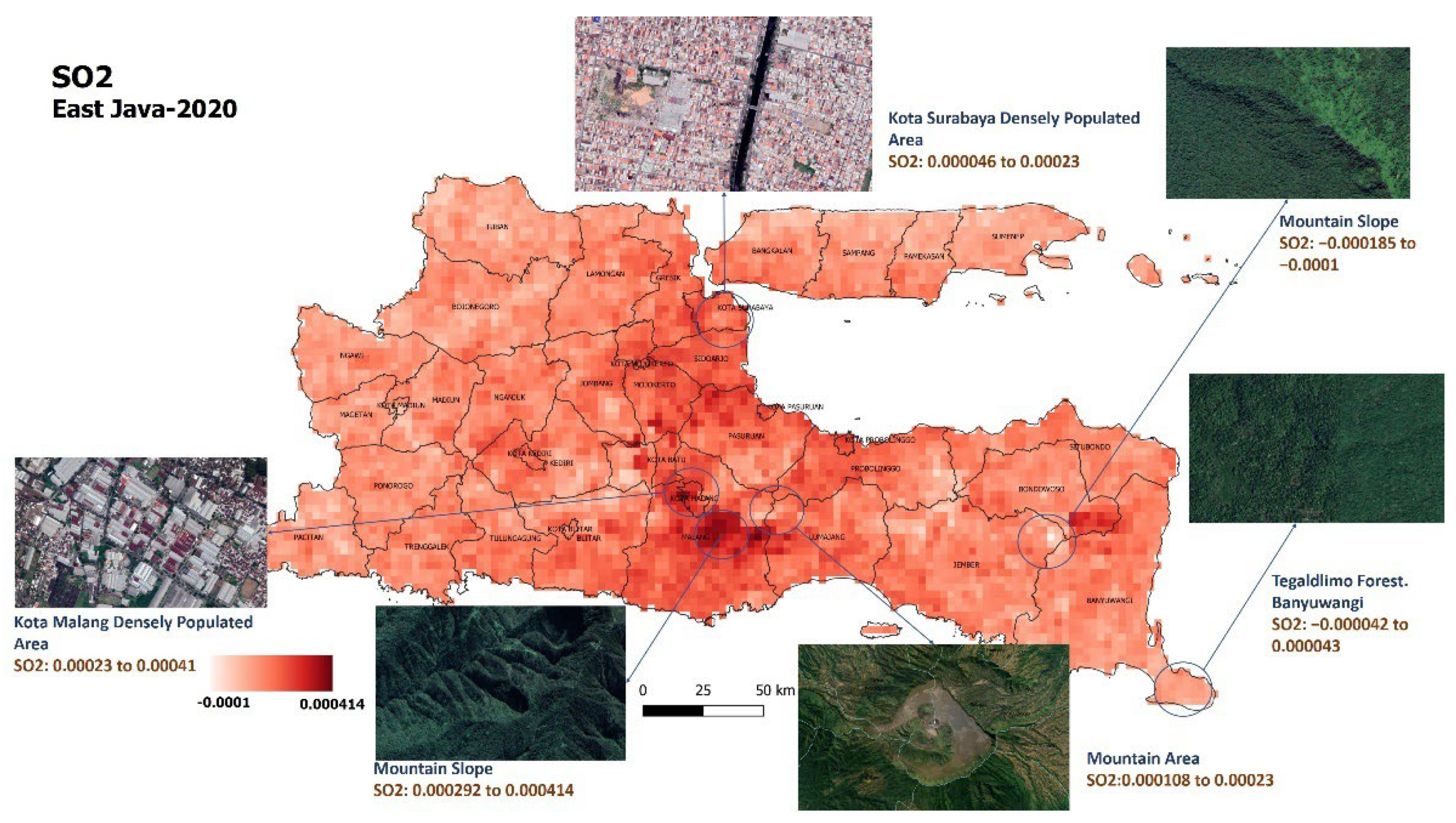
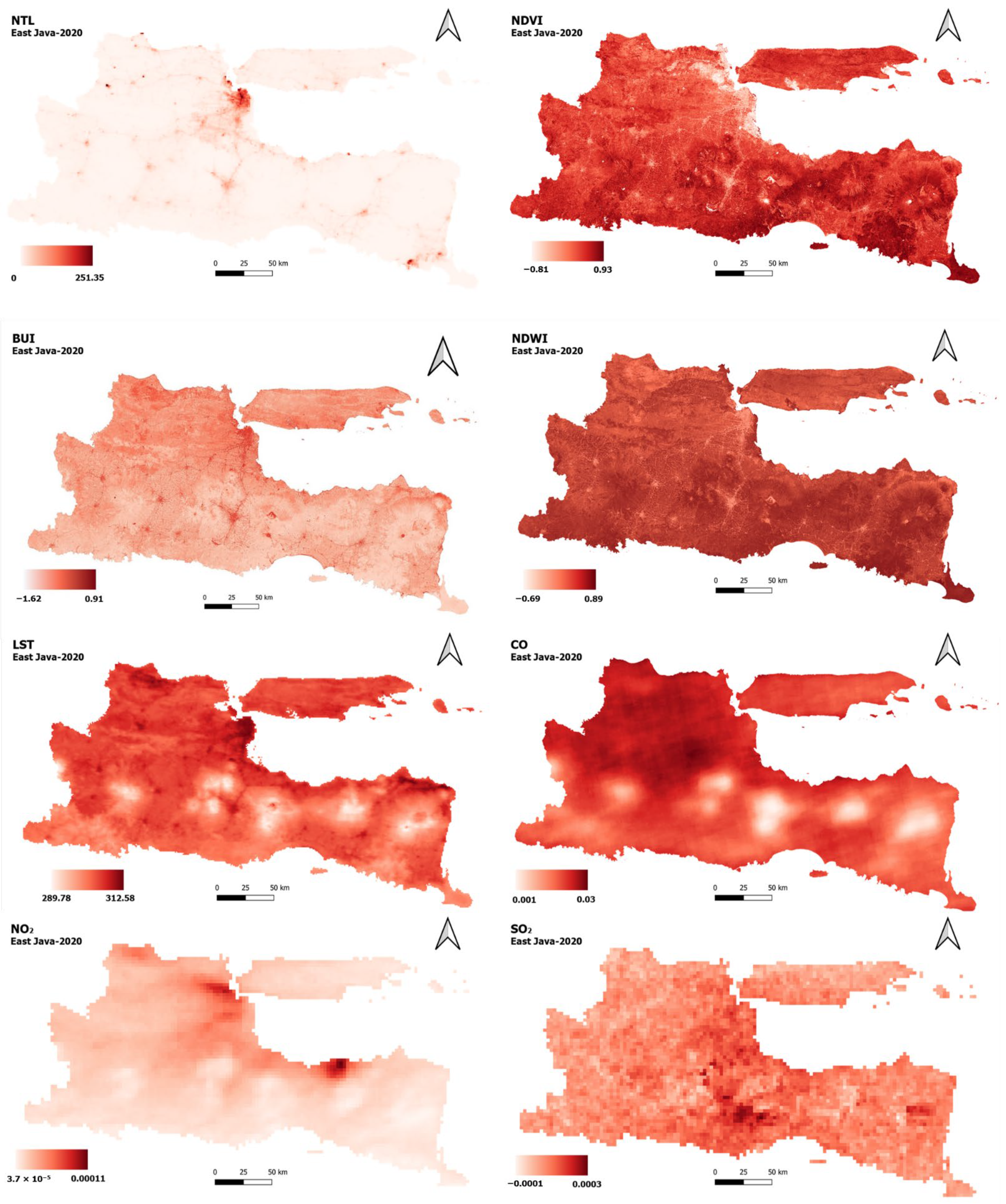
Remote-Sensing Variables Ground-Truth Check


References
- Steele, J.E.; Sundsøy, P.R.; Pezzulo, C.; Alegana, V.A.; Bird, T.J.; Blumenstock, J.; Bjelland, J.; Engø-Monsen, K.; de Montjoye, Y.-A.; Iqbal, A.M.; et al. Mapping Poverty Using Mobile Phone and Satellite Data. R. Soc. 2017, 14, 20160690. [Google Scholar] [CrossRef] [PubMed]
- United Nations End Poverty in All Its Forms Everywhere. Available online: https://unstats.un.org/sdgs/report/2020/goal-01/ (accessed on 23 December 2021).
- United Nations Ending Poverty. Available online: https://www.un.org/en/global-issues/ending-poverty (accessed on 1 March 2022).
- United Nations about the Sustainable Development Goals. Available online: https://www.un.org/sustainabledevelopment/sustainable-development-goals/ (accessed on 23 December 2021).
- Zhao, X.; Yu, B.; Liu, Y.; Chen, Z.; Li, Q.; Wang, C.; Wu, J. Estimation of Poverty Using Random Forest Regression with Multi-Source Data: A Case Study in Bangladesh. Remote Sens. 2019, 11, 375. [Google Scholar] [CrossRef] [Green Version]
- Statistics Indonesia (BPS). Regency/Municipality Poverty Data and Information in 2021; Statistics Indonesia: Jakarta, Indonesia, 2021.
- Indonesia National Development Planning Agency (Bappenas). Indonesia SDGs Roadmap Towards 2030; Indonesia National Development Planning Agency: Jakarta, Indonesia, 2017.
- Jerven, M. Benefits and Costs of the Data for Development Targets for the Post-2015 Development Agenda. Data Dev. Assess. Pap. 2014, 16, 14. [Google Scholar]
- Laurentcia, S.; Yusran, R. Evaluation of the Non-Cash Food Assistance Program in Poverty Reduction in Padang District. J. Civ. Educ. 2021, 4, 7–17. [Google Scholar] [CrossRef]
- Indonesia National Development Planning Agency (Bappenas). National Mid-Term Development Plan (RPJMN) 2020–2024; Indonesia National Development Planning Agency: Jakarta, Indonesia, 2020.
- Triscowati, D.W.; Sartono, B.; Kurnia, A.; Domiri, D.D.; Wijayanto, A.W. Multitemporal Remote Sensing Data for Classification of Food Crops Plant Phase Using Supervised Random Forest. In Proceedings of the 6th Geoinformation Science Symposium, Yogyakarta, Indonesia, 26–27 August 2019; Volume 11311, p. 1131102. [Google Scholar]
- Triscowati, D.W.; Sartono, B.; Kurnia, A.; Dirgahayu, D.; Wijayanto, A.W. Classification of Rice-Plant Growth Phase Using Supervised Random Forest Method Based on Landsat-8 Multitemporal Data. Int. J. Remote Sens. Earth Sci. 2020, 16, 187–196. [Google Scholar] [CrossRef]
- Wijayanto, A.W.; Triscowati, D.W.; Marsuhandi, A.H. Maize Field Area Detection in East Java, Indonesia: An Integrated Multispectral Remote Sensing and Machine Learning Approach. In Proceedings of the 2020 12th International Conference on Information Technology and Electrical Engineering (ICITEE), Yogyakarta, Indonesia, 6–8 October 2020; pp. 168–173. [Google Scholar]
- Shi, K.; Chang, Z.; Chen, Z.; Wu, J.; Yu, B. Identifying and Evaluating Poverty Using Multisource Remote Sensing and Point of Interest (POI) Data: A Case Study of Chongqing, China. J. Clean. Prod. 2020, 255, 120245. [Google Scholar] [CrossRef]
- Fauzi, A.I.; Sakti, A.D.; Yayusman, L.F.; Harto, A.B.; Prasetyo, L.B.; Irawan, B.; Wikantika, K. Evaluating mangrove forest deforestation causes in Southeast Asia by analyzing recent environment and socio-economic data products. In Proceedings of the 39th Asian Conference on Remote Sensing: Remote Sensing Enabling Prosperity, ACRS 2018, Kuala Lumpur, Malaysia, 15–19 October 2018; Asian Association on Remote Sensing: Kuala Lumpur, Malaysia, 2018; Volume 2, pp. 880–889. [Google Scholar]
- Pokhriyal, N.; Zambrano, O.; Linares, J.; Hernández, H. Estimating and Forecasting Income Poverty and Inequality in Haiti Using Satellite Imagery and Mobile Phone Data; Inter-American Development Bank: Washington, DC, USA, 2020. [Google Scholar]
- Ghosh, T.; Anderson, S.J.; Elvidge, C.D.; Sutton, P.C. Using Nighttime Satellite Imagery as a Proxy Measure of Human Well-Being. Sustainability 2013, 5, 4988–5019. [Google Scholar] [CrossRef] [Green Version]
- Rajagukguk, Y.S.; Sakti, A.D.; Yayusman, L.F.; Harto, A.B.; Prasetyo, L.B.; Irawan, B.; Wikantika, K. Evaluation of Southeast Asia mangrove forest deforestation using longterm remote sensing index datasets. In Proceedings of the 39th Asian Conference on Remote Sensing: Remote Sensing Enabling Prosperity, ACRS 2018, Kuala Lumpur, Malaysia, 15–19 October 2018; Asian Association on Remote Sensing: Kuala Lumpur, Malaysia, 2018; Volume 2, pp. 931–937. [Google Scholar]
- Zhao, N.; Liu, Y.; Cao, G.; Samson, E.L.; Zhang, J. Forecasting China’s GDP at the Pixel Level Using Nighttime Lights Time Series and Population Images. GISci. Remote Sens. 2017, 54, 407–425. [Google Scholar] [CrossRef]
- Shi, K.; Yu, B.; Huang, Y.; Hu, Y.; Yin, B.; Chen, Z.; Chen, L.; Wu, J. Evaluating the Ability of NPP-VIIRS Nighttime Light Data to Estimate the Gross Domestic Product and the Electric Power Consumption of China at Multiple Scales: A Comparison with DMSP-OLS Data. Remote Sens. 2014, 6, 1705–1724. [Google Scholar] [CrossRef] [Green Version]
- Putri, S.R.; Suganda, T.G.; Pramana, S. Bayesian Network Implementation for Modelling Indonesia’s Green Economy Condition Based on Big Data. In Proceedings of the Seminar Nasional Official Statistics, Jakarta, Indonesia, 25 September 2021; Volume 2021, pp. 1054–1064. [Google Scholar]
- Sakti, A.D.; Rinasti, A.N.; Agustina, E.; Diastomo, H.; Muhammad, F.; Anna, Z.; Wikantika, K. Multi-Scenario Model of Plastic Waste Accumulation Potential in Indonesia Using Integrated Remote Sensing, Statistic and Socio-Demographic Data. ISPRS Int. J. Geo-Inf. 2021, 10, 481. [Google Scholar] [CrossRef]
- Chen, Z.; Yu, B.; Hu, Y.; Huang, C.; Shi, K.; Wu, J. Estimating House Vacancy Rate in Metropolitan Areas Using NPP-VIIRS Nighttime Light Composite Data. IEEE J. Sel. Top. Appl. Earth Obs. Remote Sens. 2015, 8, 2188–2197. [Google Scholar] [CrossRef]
- Shi, K.; Yang, Q.; Fang, G.; Yu, B.; Chen, Z.; Yang, C.; Wu, J. Evaluating Spatiotemporal Patterns of Urban Electricity Consumption within Different Spatial Boundaries: A Case Study of Chongqing, China. Energy 2019, 167, 641–653. [Google Scholar] [CrossRef]
- Sutton, P.; Roberts, D.; Elvidge, C.; Baugh, K. Census from Heaven: An Estimate of the Global Human Population Using Night-Time Satellite Imagery. Int. J. Remote Sens. 2001, 22, 3061–3076. [Google Scholar] [CrossRef]
- Shi, K.; Yu, B.; Hu, Y.; Huang, C.; Chen, Y.; Huang, Y.; Chen, Z.; Wu, J. Modeling and Mapping Total Freight Traffic in China Using NPP-VIIRS Nighttime Light Composite Data. GISci. Remote Sens. 2015, 52, 274–289. [Google Scholar] [CrossRef]
- Elvidge, C.D.; Sutton, P.C.; Ghosh, T.; Tuttle, B.T.; Baugh, K.E.; Bhaduri, B.; Bright, E. A Global Poverty Map Derived from Satellite Data. Comput. Geosci. 2009, 35, 1652–1660. [Google Scholar] [CrossRef]
- Yu, B.; Tang, M.; Wu, Q.; Yang, C.; Deng, S.; Shi, K.; Peng, C.; Wu, J.; Chen, Z. Urban Built-up Area Extraction from Log-Transformed NPP-VIIRS Nighttime Light Composite Data. IEEE Geosci. Remote Sens. Lett. 2018, 15, 1279–1283. [Google Scholar] [CrossRef]
- Yin, J.; Qiu, Y.; Zhang, B. Identification of Poverty Areas by Remote Sensing and Machine Learning: A Case Study in Guizhou, Southwest China. ISPRS Int. J. Geo-Inf. 2020, 10, 11. [Google Scholar] [CrossRef]
- Sapena, M.; Ruiz, L.A.; Taubenböck, H. Analyzing Links between Spatio-Temporal Metrics of Built-up Areas and Socio-Economic Indicators on a Semi-Global Scale. ISPRS Int. J. Geo-Inf. 2020, 9, 436. [Google Scholar] [CrossRef]
- Tian, Y.; Wang, Z.; Zhao, J.; Jiang, X.; Guo, R. A Geographical Analysis of the Poverty Causes in China’s Contiguous Destitute Areas. Sustainability 2018, 10, 1895. [Google Scholar] [CrossRef] [Green Version]
- Dawson, T.; Sandoval, J.S.; Sagan, V.; Crawford, T. A Spatial Analysis of the Relationship between Vegetation and Poverty. ISPRS Int. J. Geo-Inf. 2018, 7, 83. [Google Scholar] [CrossRef] [Green Version]
- Kaimaris, D.; Patias, P. Identification and Area Measurement of the Built-up Area with the Built-up Index (BUI). Int. J. Adv. Remote Sens. GIS 2016, 5, 1844–1858. [Google Scholar] [CrossRef] [Green Version]
- Alkire, S.; Chatterje, M.; Conconi, A.; Seth, S.; Vaz, A. Poverty in Rural and Urban Areas: Direct Comparisons Using the Global MPI 2014. Briefing 2014. [Google Scholar] [CrossRef]
- Huang, G.; Zhou, W.; Cadenasso, M.L. Is Everyone Hot in the City? Spatial Pattern of Land Surface Temperatures, Land Cover and Neighborhood Socioeconomic Characteristics in Baltimore, MD. J. Environ. Manag. 2011, 92, 1753–1759. [Google Scholar] [CrossRef] [PubMed]
- Ahmed, S. Assessment of Urban Heat Islands and Impact of Climate Change on Socioeconomic over Suez Governorate Using Remote Sensing and GIS Techniques. Egypt. J. Remote Sens. Space Sci. 2018, 21, 15–25. [Google Scholar] [CrossRef]
- Zheng, Y.; Zhou, Q.; He, Y.; Wang, C.; Wang, X.; Wang, H. An Optimized Approach for Extracting Urban Land Based on Log-Transformed DMSP-OLS Nighttime Light, NDVI, and NDWI. Remote Sens. 2021, 13, 766. [Google Scholar] [CrossRef]
- Baloch, M.A.; Khan, S.U.-D.; Ulucak, Z.S.; Ahmad, A. Analyzing the Relationship between Poverty, Income Inequality, and CO2 Emission in Sub-Saharan African Countries. Sci. Total Environ. 2020, 740, 139867. [Google Scholar] [CrossRef]
- Sakti, A.D.; Fauzi, A.I.; Takeuchi, W.; Pradhan, B.; Yarime, M.; Vega-Garcia, C.; Agustina, E.; Wibisono, D.; Anggraini, T.S.; Theodora, M.O.; et al. Spatial Prioritization for Wildfire Mitigation by Integrating Heterogeneous Spatial Data: A New Multi-Dimensional Approach for Tropical Rainforests. Remote Sens. 2022, 14, 543. [Google Scholar] [CrossRef]
- Wang, Y.; Li, J.; Wang, L.; Lin, Y.; Zhou, M.; Yin, P.; Yao, S. The Impact of Carbon Monoxide on Years of Life Lost and Modified Effect by Individual-and City-Level Characteristics: Evidence from a Nationwide Time-Series Study in China. Ecotoxicol. Environ. Saf. 2021, 210, 111884. [Google Scholar] [CrossRef]
- Sakti, A.D.; Rahadianto, M.A.E.; Pradhan, B.; Muhammad, H.N.; Andani, I.G.A.; Sarli, P.W.; Abdillah, M.R.; Anggraini, T.S.; Purnomo, A.D.; Ridwana, R.; et al. School Location Analysis by Integrating the Accessibility, Natural and Biological Hazards to Support Equal Access to Education. ISPRS Int. J. Geo-Inf. 2022, 11, 12. [Google Scholar] [CrossRef]
- Han, C.; Gu, Z.; Yang, H. EKC Test of the Relationship between Nitrogen Dioxide Pollution and Economic Growth—A Spatial Econometric Analysis Based on Chinese City Data. Int. J. Environ. Res. Public Health 2021, 18, 9697. [Google Scholar] [CrossRef]
- Bakhsh, K.; Akmal, T.; Ahmad, T.; Abbas, Q. Investigating the Nexus among Sulfur Dioxide Emission, Energy Consumption, and Economic Growth: Empirical Evidence from Pakistan. Environ. Sci. Pollut. Res. 2022, 29, 7214–7224. [Google Scholar] [CrossRef] [PubMed]
- Duque, J.C.; Patino, J.E.; Ruiz, L.A.; Pardo-Pascual, J.E. Measuring Intra-Urban Poverty Using Land Cover and Texture Metrics Derived from Remote Sensing Data. Landsc. Urban Plan. 2015, 135, 11–21. [Google Scholar] [CrossRef]
- Sakti, A.D.; Tsuyuki, S. Spectral Mixture Analysis of Peatland Imagery for Land Cover Study of Highly Degraded Peatland in Indonesia. In The International Archives of the Photogrammetry, Remote Sensing and Spatial Information Science; Copernicus Publications: Göttingen, Germany, 2015; Volume XL-7/W3. [Google Scholar]
- Niu, T.; Chen, Y.; Yuan, Y. Measuring Urban Poverty Using Multi-Source Data and a Random Forest Algorithm: A Case Study in Guangzhou. Sustain. Cities Soc. 2020, 54, 102014. [Google Scholar] [CrossRef]
- Zhou, Y.; Liu, Y. The geography of poverty: Review and research prospects. J. Rural Stud. 2019. in press. Available online: https://www.sciencedirect.com/science/article/abs/pii/S0743016718303899 (accessed on 30 September 2021). [CrossRef]
- Statistics Indonesia (BPS). Regency/Municipality Poverty Data and Information in 2020; Statistics Indonesia: Jakarta, Indonesia, 2020.
- Wasonowati, C.; Sulistyaningsih, E.; Indradewa, D.; Kurniasih, B. Physiological Characters of Moringa Oleifera Lamk in Madura. In AIP Conference Proceedings; American Institute of Physics: University Park, MD, USA, 2019; Volume 2120, p. 30024. [Google Scholar]
- Wisnubroto, E.I.; Rustiadi, E.; Fauzi, A.; Murtilaksono, K. The Dynamic Changes in Peri-Urban Agricultural Area and Typology of Multi-Function Agriculture in Batu City, Indonesia. IOP Conf. Ser. Earth Environ. Sci. 2021, 667, 12093. [Google Scholar] [CrossRef]
- Setiawan, F.C.; Rahadian, S. Social, Cultural and Political Conditions in Malang Before Kanjuruhan Kingdom. Soc. Sci. Stud. Sustain. ISSUES 2019, 63, 63–69. [Google Scholar]
- Santoso, E.B.; Aulia, B.U. Ecological Sustainability Level of Surabaya City Based on Ecological Footprint Approach. IOP Conf. Ser. Earth Environ. Sci. 2018, 202, 12044. [Google Scholar] [CrossRef]
- Nurmasari, Y.; Wijayanto, A.W. Oil Palm Plantation Detection in Indonesia Using Sentinel-2 and Landsat-8 Optical Satellite Imagery (Case Study: Rokan Hulu Regency, Riau Province). Int. J. Remote Sens. Earth Sci. 2021, 18, 1–18. [Google Scholar] [CrossRef]
- Saadi, T.D.T.; Wijayanto, A.W. Machine Learning Applied to Sentinel-2 and Landsat-8 Multispectral and Medium-Resolution Satellite Imagery for the Detection of Rice Production Areas in Nganjuk, East Java, Indonesia. Int. J. Remote Sens. Earth Sci. 2021, 18, 19–32. [Google Scholar]
- Putri, S.R.; Wijayanto, A.W. Learning Bayesian Network for Rainfall Prediction Modeling in Urban Area Using Remote Sensing Satellite Data (Case Study: Jakarta, Indonesia). In Proceedings of the International Conference on Data Science and Official Statistics, Online, 13–14 November 2021; Volume 2021, pp. 77–90. [Google Scholar]
- Tingzon, I.; Orden, A.; Sy, S.; Sekara, V.; Weber, I.; Fatehkia, M.; Garcia, M.; Dohyung, H. Mapping Poverty in the Philippines Using Machine Learning, Satellite Imagery, and Crowd-Sourced Geospatial Information. SPRS-Int. Arch. Photogramm. Remote Sens. Spat. Inf. Sci. 2019, 42, 425–431. [Google Scholar] [CrossRef] [Green Version]
- Ledesma, C.; Garonita, O.L.; Flores, L.J.; Tingzon, I.; Dalisay, D. Interpretable Poverty Mapping Using Social Media Data, Satellite Images, and Geospatial Information. arXiv 2020, arXiv:2011.13563. [Google Scholar]
- Earth Observation Group Payne Institute for Public Policy Colorado School of Mines VIIRS Nighttime Day/Night Band Composites Version 1. Available online: https://developers.google.com/earth-engine/datasets/catalog/NOAA_VIIRS_DNB_MONTHLY_V1_VCMCFG (accessed on 10 September 2021).
- Zhao, N.; Cao, G.; Zhang, W.; Samson, E.L.; Chen, Y. Remote Sensing and Social Sensing for Socioeconomic Systems: A Comparison Study between Nighttime Lights and Location-Based Social Media at the 500 m Spatial Resolution. Int. J. Appl. Earth Obs. Geoinf. 2020, 87, 102058. [Google Scholar] [CrossRef]
- Zhou, N.; Hubacek, K.; Roberts, M. Analysis of Spatial Patterns of Urban Growth across South Asia Using DMSP-OLS Nighttime Lights Data. Appl. Geogr. 2015, 63, 292–303. [Google Scholar] [CrossRef]
- Copernicus ESA European Union Sentinel-2 MSI: MultiSpectral Instrument, Level-2A. Available online: https://developers.google.com/earth-engine/datasets/catalog/COPERNICUS_S2_SR (accessed on 10 September 2021).
- Purevdorj, T.S.; Tateishi, R.; Ishiyama, T.; Honda, Y. Relationships between Percent Vegetation Cover and Vegetation Indices. Int. J. Remote Sens. 1998, 19, 3519–3535. [Google Scholar] [CrossRef]
- Lee, J.; Lee, S.S.; Chi, K.H. Development of an Urban Classification Method Using a Built-up Index. In Proceedings of the 6th WSEAS International Conference on Remote Sensing, Takizawa, Japan, 4–6 October 2010; pp. 39–43. [Google Scholar]
- McFeeters, S.K. The Use of the Normalized Difference Water Index (NDWI) in the Delineation of Open Water Features. Int. J. Remote Sens. 1996, 17, 1425–1432. [Google Scholar] [CrossRef]
- NASA LP DAAC at the USGS EROS Center MOD11A1.006 Terra Land Surface Temperature and Emissivity Daily Global 1 km. Available online: https://developers.google.com/earth-engine/datasets/catalog/MODIS_006_MOD11A1 (accessed on 15 September 2021).
- Copernicus ESA European Union Sentinel-5P OFFL CO: Offline Carbon Monoxide. Available online: https://developers.google.com/earth-engine/datasets/catalog/COPERNICUS_S5P_OFFL_L3_CO (accessed on 10 September 2021).
- Copernicus ESA European Union Sentinel-5P OFFL NO2: Offline Nitrogen Dioxide. Available online: https://developers.google.com/earth-engine/datasets/catalog/COPERNICUS_S5P_OFFL_L3_NO2?hl=en (accessed on 10 September 2021).
- Copernicus ESA European Union Sentinel-5P OFFL SO2: Offline Sulphur Dioxide. Available online: https://developers.google.com/earth-engine/datasets/catalog/COPERNICUS_S5P_OFFL_L3_SO2 (accessed on 10 September 2021).
- Open StreetMap Open StreetMap. Available online: https://www.openstreetmap.org/ (accessed on 15 July 2020).
- Tamilselvi, R.; Sivasakthi, B.; Kavitha, R. An Efficient Preprocessing and Postprocessing Techniques in Data Mining. Int. J. Res. Comput. Appl. Robot. 2015, 3, 80–85. [Google Scholar]
- Fauzi, A.I.; Sakti, A.D.; Robbani, B.F.; Ristiyani, M.; Agustin, R.T.; Yati, E.; Nuha, M.U.; Anika, N.; Putra, R.; Siregar, D.I.; et al. Assessing Potential Climatic and Human Pressures in Indonesian Coastal Ecosystems Using a Spatial Data-Driven Approach. ISPRS Int. J. Geo-Inf. 2021, 10, 778. [Google Scholar] [CrossRef]
- Zha, Y.; Gao, J.; Ni, S. Use of Normalized Difference Built-up Index in Automatically Mapping Urban Areas from TM Imagery. Int. J. Remote Sens. 2003, 24, 583–594. [Google Scholar] [CrossRef]
- Raymaekers, J.; Rousseeuw, P.J. Transforming Variables to Central Normality. Mach. Learn. 2021, 1–23. [Google Scholar] [CrossRef]
- Sugiyono. Educational Research Methods: Quantitative, Qualitative and R&D Approaches; Alfabeta: Bandung, Indonesia, 2010. [Google Scholar]
- Wang, B.; Tian, J.; Yang, P.; He, B. Multi-Scale Features of Regional Poverty and the Impact of Geographic Capital: A Case Study of Yanbian Korean Autonomous Prefecture in Jilin Province, China. Land 2021, 10, 1406. [Google Scholar] [CrossRef]
- Liu, Y.; Xu, Y. A Geographic Identification of Multidimensional Poverty in Rural China under the Framework of Sustainable Livelihoods Analysis. Appl. Geogr. 2016, 73, 62–76. [Google Scholar] [CrossRef]
- Wang, Y.; Chen, Y. Using VPI to Measure Poverty-Stricken Villages in China. Soc. Indic. Res. 2017, 133, 833–857. [Google Scholar] [CrossRef]
- Goyal, M.K.; Singh, V.; Meena, A.H. Geospatial and Hydrological Modeling to Assess Hydropower Potential Zones and Site Location over Rainfall Dependent Inland Catchment. Water Resour. Manag. 2015, 29, 2875–2894. [Google Scholar] [CrossRef]
- Uddin, M.N.; Islam, A.K.M.S.; Bala, S.K.; Islam, G.M.T.; Adhikary, S.; Saha, D.; Haque, S.; Fahad, M.G.R.; Akter, R. Mapping of Climate Vulnerability of the Coastal Region of Bangladesh Using Principal Component Analysis. Appl. Geogr. 2019, 102, 47–57. [Google Scholar] [CrossRef]
- Cartone, A.; Postiglione, P. Principal Component Analysis for Geographical Data: The Role of Spatial Effects in the Definition of Composite Indicators. Spat. Econ. Anal. 2021, 16, 126–147. [Google Scholar] [CrossRef]
- Sakti, A.D.; Takeuchi, W. A data-intensive approach to address food sustainability: Integrating optic and microwave satellite imagery for developing long-term global cropping intensity and sowing month from 2001 to 2015. Sustainability 2020, 12, 3227. [Google Scholar] [CrossRef] [Green Version]
- Varshney, K.R.; Chen, G.H.; Abelson, B.; Nowocin, K.; Sakhrani, V.; Xu, L.; Spatocco, B.L. Targeting Villages for Rural Development Using Satellite Image Analysis. Big Data 2015, 3, 41–53. [Google Scholar] [CrossRef] [PubMed] [Green Version]
- Assael, H.; Keon, J. Nonsampling vs. Sampling Errors in Survey Research. J. Mark. 1982, 46, 114–123. [Google Scholar] [CrossRef]
- Sarmah, H.K.; Hazarika, B.B.; Choudhury, G. An Investigation on Effect of Bias on Determination of Sample Size on the Basis of Data Related to the Students of Schools of Guwahati. Int. J. Appl. Math. Stat. Sci. 2013, 2, 33–48. [Google Scholar]
- Sari, F.E.K.; Fitria, I.; Hariyanto, D.D.; Fachriansyah, M.A. Internship Lecture Report Analysis of Internal Control Activities of the National Socio-Economic Survey (Susenas) Central Bureau of Statistics Jombang Regency; STIE PGRI Dewantara: Surabaya, Indonesia, 2019. [Google Scholar]
- Afifah, U.N.; Faradis, R. Sosial Ekonomi Nasional Survey (Susenas) Data Optimization with Small Area Estimation (SAE) Case Study: Village Level Proverty Estimation in Belitung Timur Regency. In Proceedings of the Seminar Nasional Official Statistics, Jakarta, Indonesia, 24 September 2019; Volume 2019, pp. 132–139. [Google Scholar]
- Chakravarty, S.R.; Deutsch, J.; Silber, J. On the Watts Multidimensional Poverty Index and Its Decomposition. World Dev. 2008, 36, 1067–1077. [Google Scholar] [CrossRef]
- Jalan, J.; Ravallion, M. Geographic Poverty Traps? A Micro Model of Consumption Growth in Rural China. J. Appl. Econom. 2002, 17, 329–346. [Google Scholar] [CrossRef] [Green Version]
- Grant, U. The Chronic Poverty Report 2004–2005; Institute for Development Policy & Management, University of Manchester: Manchester, UK, 2004. [Google Scholar]
- Addison, T.; Harper, C.; Prowse, M.; Shepherd, A.; Barrientos, A.; Braunholtz-Speight, T.; Evans, A.; Grant, U.; Hickey, S.; Hulme, D.; et al. The Chronic Poverty Report 2008–2009: Escaping Poverty Traps. Eur. J. Dev. Res. 2008, 21, 159. [Google Scholar]
- Maurya, R.; Gupta, P.R.; Shukla, A.S.; Sharma, M.K. Building Extraction from Very High Resolution Multispectral Images Using NDVI Based Segmentation and Morphological Operators. In Proceedings of the IEEE-International Conference on Advances In Engineering, Science and Management (ICAESM-2012), Nagapattinam, India, 30–31 March 2012; pp. 577–581. [Google Scholar]
- Mia, B.; Bhattacharya, R.; Woobaidullah, A.S.M. Correlation and Monitoring of Land Surface Temperature, Urban Heat Island with Land Use-Land Cover of Dhaka City Using Satellite Imageries. Int. J. Res. Geogr. 2017, 3, 10–20. [Google Scholar]
- Wu, J.; He, L.-Y.; Zhang, Z. Does China Fall into Poverty-Environment Traps? Evidence from Long-Term Income Dynamics and Urban Air Pollution. FEEM Work. Pap. 2019, 5, 1–27. [Google Scholar]


| Source | Spatial Resolution | Variable | Band Used | Year Data Analysis | Units | Socio-Economic References |
|---|---|---|---|---|---|---|
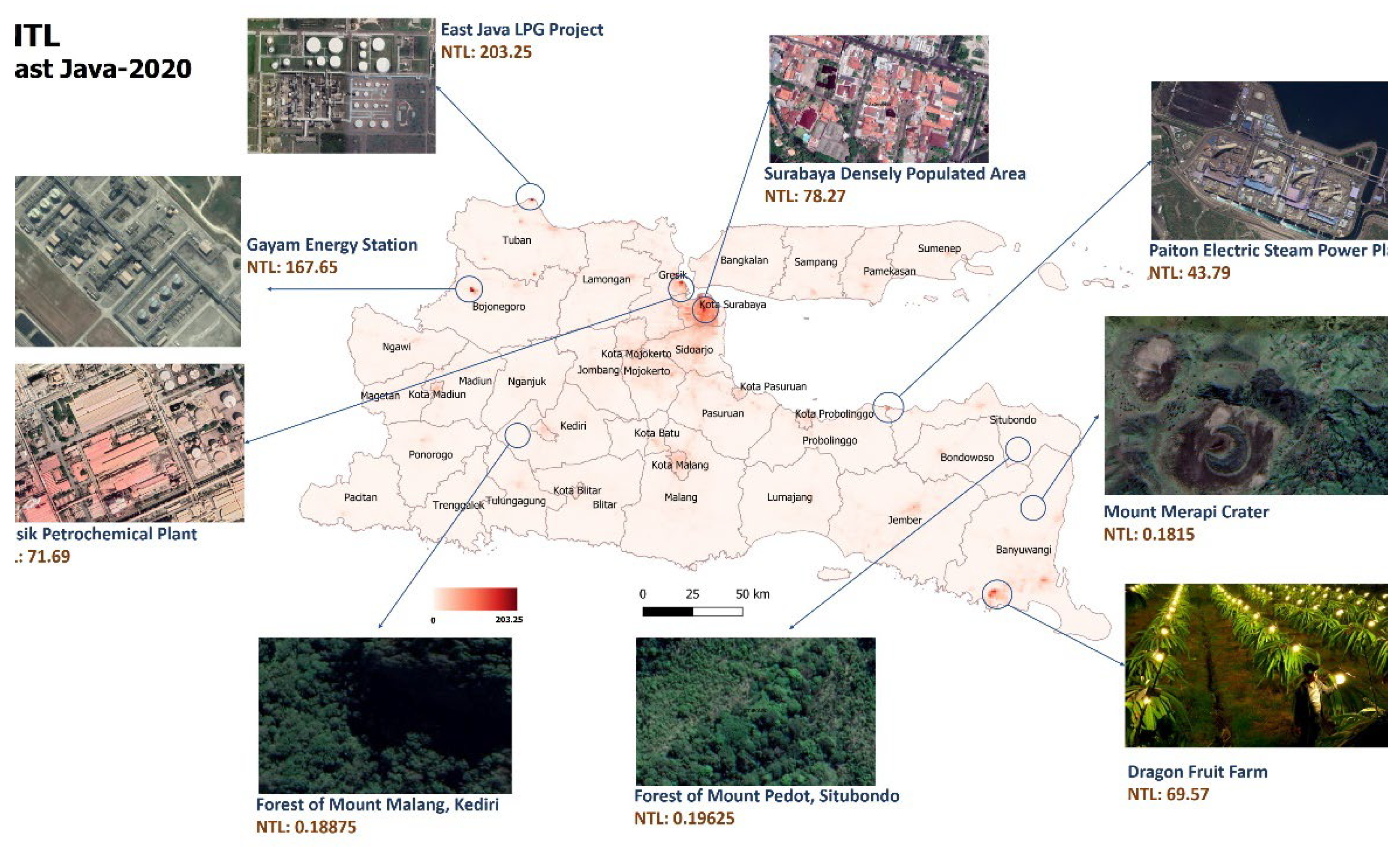
| NOAA-VIIRS [58] | 750 m | Night-time Light Intensity (NTL) | avg_rad | One-year NTL value | nanowatts/ cm2/sr | [17,24,25,26,27,28,59,60] |
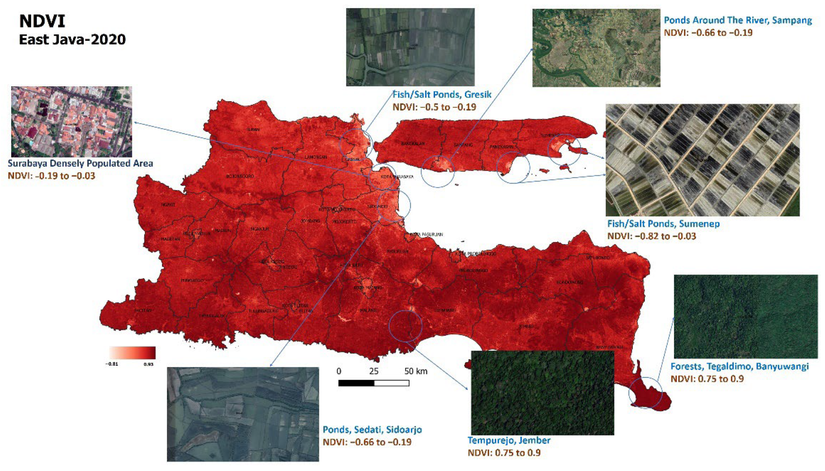
| Sentinel-2 [61] | 10 m | Normalized Difference Vegetation Index (NDVI) [62] | B4 (Red) and B8 (NIR) | The median value of 2315 cloud masked images. | index | [32,36,37] |
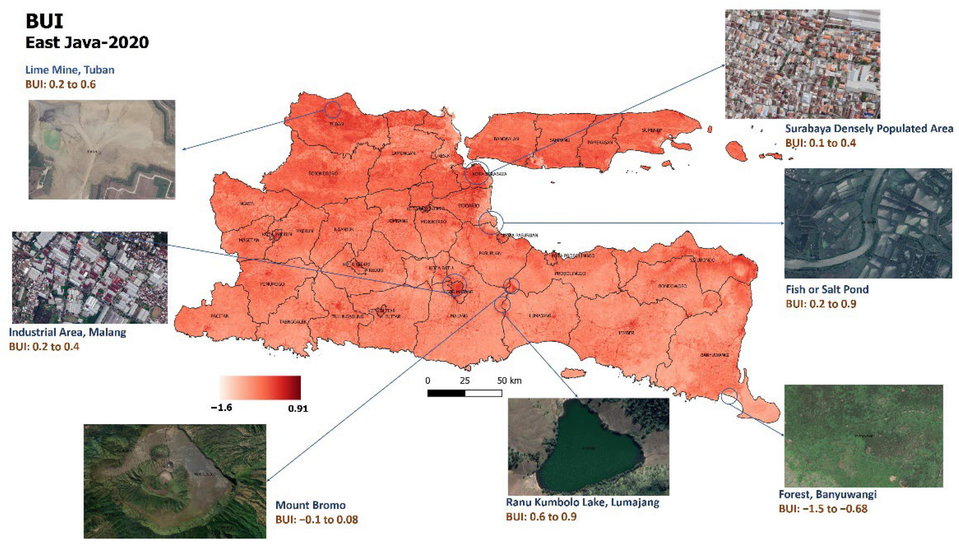
| Built-Up Index (BUI) [63] | B4 (Red), B8 (NIR), and B11 (SWIR 1) | index | [33,63] | |||
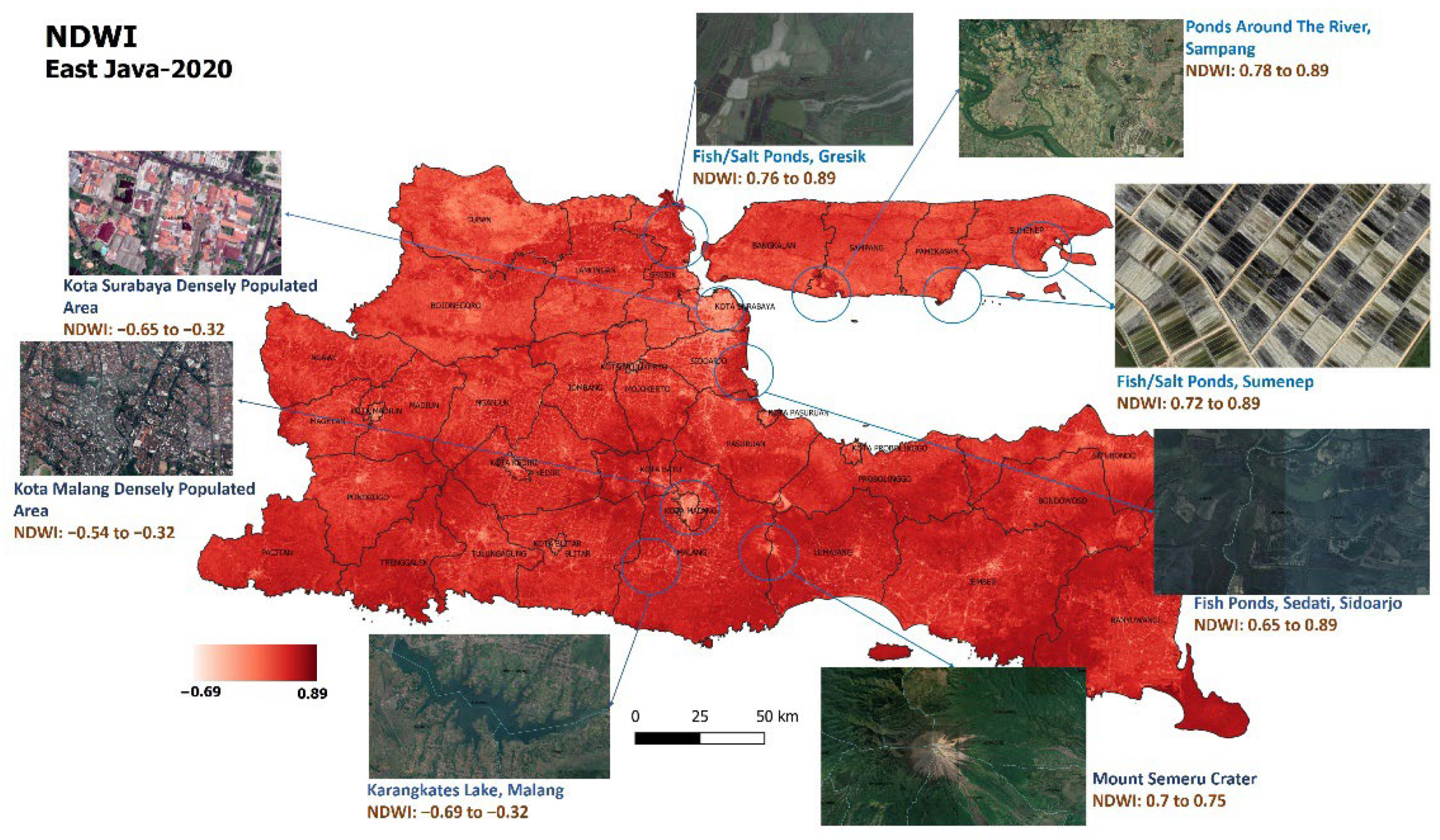
| Normalized Difference Water Index (NDWI) [64] | B3 (Green) and B8 (NIR) | index | [36,37] | |||
| MODIS [65] | 1000 m | Land Surface Temperature (LST) | LST_Day_1 km | The median value of 365 cloud-masked images. | Kelvin | [35,36] |
| Sentinel-5P [66,67,68] | 1113.2 m | Carbon Monoxide (CO) | CO column number density | The median value of the obtained images in 2020. | mol/m2 | [40] |
| Nitrogen Dioxide (NO2) | NO2 column number density | mol/m2 | [42] | |||
| Sulfur Dioxide (SO2) | SO2 column number density | mol/m2 | [43] | |||
| Open Street Map [69] | - | POI Density | - | The number of points in a 1.5 km × 1.5 km grid. | points | [14] |
| - | POI Distance | - | The distance from the center of the 1.5 km × 1.5 km grid to the nearest point. | meter | [56,57] |
| Satellite Data Source | Band | Value |
|---|---|---|
| Sentinel-2 | QA60 | Bit 10 (opaque clouds) equal 0 Bit 11 (cirrus clouds) equal 0 |
| MODIS Terra LST Daily | QC_Day | Bits 0–1 (Mandatory QA flags) equal 0 |
| Correlation Coefficient | Interpretation |
|---|---|
| Very Weak | |
| Weak | |
| Moderate | |
| Strong | |
| Very Strong |
| Variable | Pearson Correlation | Spearman Rank Correlation | Closeness | Direction | Statistically Significant | ||
|---|---|---|---|---|---|---|---|
| Correlation Coefficient | p-Value | Correlation Coefficient | p-Value | ||||
| NTL | −0.5 | 0.001 | −0.49 | 0.001 | Moderate | Negative | Yes |
| NDVI | 0.25 | 0.130 | 0.21 | 0.205 | Weak | Positive | No |
| BUI | −0.45 | 0.004 | −0.44 | 0.005 | Moderate | Negative | Yes |
| NDWI | 0.14 | 0.401 | 0.14 | 0.401 | Weak | Positive | No |
| LST | −0.29 | 0.077 | −0.31 | 0.058 | Weak | Negative | No |
| CO | −0.065 | 0.698 | −0.054 | 0.747 | Very Weak | Negative | No |
| NO2 | −0.25 | 0.130 | −0.26 | 0.114 | Weak | Negative | No |
| SO2 | −0.6 | −0.63 | Strong | Negative | Yes | ||
| POI Density | −0.64 | −0.72 | Strong | Negative | Yes | ||
| POI Distance | 0.73 | 0.79 | Strong | Positive | Yes | ||
| Variable | ||
|---|---|---|
| NTL | −0.5 | 0.5 |
| BUI | −0.45 | 0.26 |
| SO2 | −0.6 | 0.29 |
| POI Density | −0.64 | 0.5 |
| POI Distance | 0.75 | 0.58 |
| Index | Pearson Correlation | Spearman Rank Correlation | Closeness | Direction | Statistically Significant | ||
|---|---|---|---|---|---|---|---|
| Correlation Coefficient | p-Value | Correlation Coefficient | p-Value | ||||
| 0.71 | 0.77 | Strong | Positive | Yes | |||
| 0.69 | 0.72 | Strong | Positive | Yes | |||
| Model | ||
| RMSE | 3.18% | 3.25% |
| 0.50 | 0.48 |
Publisher’s Note: MDPI stays neutral with regard to jurisdictional claims in published maps and institutional affiliations. |
© 2022 by the authors. Licensee MDPI, Basel, Switzerland. This article is an open access article distributed under the terms and conditions of the Creative Commons Attribution (CC BY) license (https://creativecommons.org/licenses/by/4.0/).
Share and Cite
Putri, S.R.; Wijayanto, A.W.; Sakti, A.D. Developing Relative Spatial Poverty Index Using Integrated Remote Sensing and Geospatial Big Data Approach: A Case Study of East Java, Indonesia. ISPRS Int. J. Geo-Inf. 2022, 11, 275. https://doi.org/10.3390/ijgi11050275
Putri SR, Wijayanto AW, Sakti AD. Developing Relative Spatial Poverty Index Using Integrated Remote Sensing and Geospatial Big Data Approach: A Case Study of East Java, Indonesia. ISPRS International Journal of Geo-Information. 2022; 11(5):275. https://doi.org/10.3390/ijgi11050275
Chicago/Turabian StylePutri, Salwa Rizqina, Arie Wahyu Wijayanto, and Anjar Dimara Sakti. 2022. "Developing Relative Spatial Poverty Index Using Integrated Remote Sensing and Geospatial Big Data Approach: A Case Study of East Java, Indonesia" ISPRS International Journal of Geo-Information 11, no. 5: 275. https://doi.org/10.3390/ijgi11050275
APA StylePutri, S. R., Wijayanto, A. W., & Sakti, A. D. (2022). Developing Relative Spatial Poverty Index Using Integrated Remote Sensing and Geospatial Big Data Approach: A Case Study of East Java, Indonesia. ISPRS International Journal of Geo-Information, 11(5), 275. https://doi.org/10.3390/ijgi11050275