Managing Inhomogeneity in the Control Point Network during Staking Out Cadastral Boundaries in Austria

Abstract

The coordinate system of the Austrian cadastre is physically realised through control points provided by the national institution for surveying. Due to historical development over the centuries and changes in measurement technologies, inhomogeneities can occur within the local control point network. These inhomogeneities affect the derived boundary point coordinates. When staking out boundary points in an area with inhomogeneous control points, deviations from the boundary marks in the field can occur that exceed the accuracy requirements of the ordinance for surveying. Examples show that a suitable approach to tackle this issue has to be selected on a case-based strategy. Different situations might require different approaches. This needs to be considered in the legal framework to enable cadastral experts to select the optimal approach.

1. Introduction

Staking out boundary points for the purpose of marking property boundaries in the field is a frequently performed activity in any cadastre. When transferring the coordinates from a cadastral map to the field, deviations from the current location of the boundary marks may occur. In this work, deviations that are a result of strains in the network of control points are investigated. In Austria, the network of control points, as a physical representation of the national coordinate system, forms the technical basis for determining the coordinates of boundary points. Since 1817, the neighbourhood relations of the control points have shown strains, which are subsequently also transferred to the derived boundary point coordinates. Differences will arise between the coordinates of the boundary markings in the real world and those according to the legal boundary cadastre [1] when staking out boundary points from the legal boundary cadastre using the official control point network according to the current Austrian surveying ordinance (VermV2016, Vermessungsverordnung). The legal boundary cadastre was introduced in 1969 and provides a guarantee for the parcel boundaries. The coordinates of the boundary points of the land parcels are derived from the nearest control points in accordance with the surveying ordinance applicable at the time of surveying and are indicated in the surveying document.

The optimal method that should be used to obtain the best results when staking out points from old cadastral surveys in a region with an inhomogeneous control point network is still up for debate. This question is significant because legal regulations dictate technical processes for special situations. If inadequate methods have to be applied, the users of the cadastre will have to deal with possible negative consequences. This paper uses three test cases to analyse different methods for staking out points based on coordinates—or, rather, the deviations that occur when applying different methods to connect to the control point network.

Old documents contain points (boundary points, polygon points, or others, such as corners of buildings) that may still exist in the real world today. These can be used for the transformation and subsequent reconstruction of boundary points, if they are physically identical. Without identification points, the staking out of points based on coordinates is not easy. Staking out coordinates from the legal boundary cadastre is only possible if the control points originally used are still present, at the same position, and do not have large strains with adjacent control points. This is not always the case.

Possible approaches are the classical Helmert transformation with or without interpolation of the residual slacks of the control points used, the interpolation of the homogeneous vectors of the control points, or the connection to the control point network by means of GNSS RTK (Global Navigation Satellite System—Real-Time Kinematic) transformation according to VermV2016. Distance-weighted interpolation, for example, can be applied to the residual gaps or homogeneous vectors to stake out boundary points in the survey area. The official pre-transformation with Austrian-wide transformation parameters from the BEV (Federal Office of Metrology and Surveying) for the transition from ETRS89 (European Terrestrial Reference System 1989) to MGI (historical Austrian Military-Geographic Institute, Militär-Geographisches Institut) coordinates still used for the Austrian cadastre can be performed for each control point determined by GNSS measurement. The difference between the (homogeneous) ETRS coordinates transformed to MGI and the original/official (inhomogeneous) MGI coordinates can be represented as a homogeneous vector. These homogeneous vectors can also be interpolated for the survey area and thus the coordinates from the legal boundary cadastre can be staked out. The difference from the homogeneous coordinates is actually a gap vector, which is called a homogeneous vector in the following sections, as in the documents of the BEV.

The legal boundary cadastre relies on the control point network. In case of inhomogeneities in the control point network, the basis for the staking out can change due to loss or movement of control points, or new coordinates of control points due to readjustment. Thus, newly derived coordinates for boundary points may change, even if the boundary marks are physically unchanged in the real world. § 13 VermG (Austrian Survey Act) provides the possibility to correct coordinates in the legal boundary cadastre by means of an ordinance issued by the surveying office with local responsibility (out of currently 41 local surveying offices). Whether a highly inhomogeneous control point network can be invoked as a reason for a correction according to § 13(1) VermG is interpreted differently by the courts, since, as opposed to administrative bodies, they are free in the choice of evidence. In any case, § 13(4) VermG explicitly offers the possibility to correct coordinates in legal boundary cadastres by an ordinance if the control point network changes due to an adjustment to a superordinate reference frame.

The broader topic of georeferencing is not only relevant for Austria. Land movement can occur abruptly or can gradually change the position of control points. A well-documented example for the first case is the Christchurch earthquake in New Zealand in 2011 [2]. Slow land movement can happen anywhere, and affects the use of all kinds of geographical data. There are various approaches to protect land rights. Kiepke states that there are more solutions for ownership protection in the European Union than there are countries [3]. The Austrian cadastre is a case where the legal design of the solution demands a high level of positional accuracy. However, even countries using GNSS solutions as a spatial reference might be affected by land movements since they change the position of boundaries and therefore their coordinates.

2. Austrian Cadastre

The Austrian land administration system consists of the cadastre defining the parcel boundaries and the land registry connecting people and parcels by rights, restrictions, and responsibilities. The land registry is based on a title registration system. The cadastre forms the geometrical basis for the land registration. It was created in 1817, and since 1883, the data have been kept up-to-date by a continuous process of documenting boundary changes. Although parcels are shown in cadastral maps, the position of the boundary can only be determined by looking at the situation in reality, by referring, for example, to boundary stones, walls, fences, or simple extent of use. Only if these elements are non-existent are the old survey documents used to reconstruct the boundary. In 1969, the quality of legal boundary cadastres was added, where the parcel owner and all neighbours agree on the position of the boundary. The agreement is documented by a licensed surveyor, who also determines the coordinates of the boundary points. The surveying authority guarantees these points to be reconstructable if boundary marks in the field are lost [4]. The coordinates of the boundary points are then proof of the boundary itself. This requires a stable control point network, which provides the geodetic reference frame.

A triangulation network and an area-wide dense control point network based on it form the basis for the cadastre. Triangulation was performed under the Austrian–Hungarian monarchy based on seven plane coordinate systems. The scale in each of the systems was determined from already existing local baseline measurements. The triangulation points should provide a reference for subsequent graphic triangulation. Due to time restrictions, the triangulation was not performed in strictly descending order. Additionally, some triangulation points were not stabilised until decades after the measurements were taken, leading to high point losses and a lack of certainty regarding the identity of the points [5,6,7,8].

In 1917, the Gauss–Krüger projection replaced plane coordinate systems. The progressive densification of the triangulation network after the Second World War created the technical basis for the legal boundary cadastre [5,6,7,9,10,11]

Since 1953, lower-level control points have been introduced, which are not determined by triangulation. With a target control point density of 10 points per square kilometre, measurements with terrestrial methods have reached their limits. The technical advancement of photogrammetry drove the rapid densification of the control point network by means of aerial photo evaluation. From today’s point of view, the photogrammetric consolidation of the control point network is to be regarded critically, since the assumed accuracy for the point location has not been achieved and is significantly lower than required for modern cadastral surveying, as already noticed in the late 1970s ([12], p. 32).

With the first surveying law, enacted in 1968, the creation and maintenance of a close-meshed network of control points became an official task of the national survey, and the connection of cadastral surveys to the control point network became a legal obligation. The goal of the legal boundary cadastre was to create a legal and technical framework that avoids boundary disputes by replacing documents that are subject to interpretation by an objective measure in the form of coordinates. A prerequisite for the creation of the legal boundary cadastre is the availability of a sufficiently accurate control point network in the respective cadastral municipality. Due to technical progress in the field of measuring instruments, especially electronic distance measurement, the control point network has been continuously re-measured, and the coordinates of the control points have been recalculated and adjusted. There are still several thousand control points in Austria whose determination has been carried out exclusively by photogrammetry, and which are therefore also subject to random deviations up to a few decimetres. In 2000, the control point network reached a maximum number of 300,000 control points. Due to point losses, e.g., from construction activities and lack of maintenance, the number has been decreasing since then [5,8,13,14].

With the availability of high-precision positioning with satellite navigation services, ETRS89 coordinates are also determined by the BEV for all control points, which have been handed over to customers since 2011 ([14], p. 38). By using this method for coordinate determination, the existing density of the control point network is no longer required for new surveys. However, to reconstruct the control point connection from previous surveys, it is still necessary to include the location of the control points used in order to be able to comply with the neighbourhood accuracy. The contradiction between an inhomogeneous, maintenance-intensive control point network and the comparatively inexpensive homogeneous ETRS89 system confronts the BEV with the task of modernising the control point network [8]. Currently (as of October 2021), the Austrian control point network comprises 56,800 triangulation points and 153,000 lower-level control points. Of these, official ETRS89 coordinates are available for all triangulation points and for 119,000 (72.5%) lower-level points.

Until the introduction of the Austrian Survey Act on 1 January 1969, the cadastre was used to visualise parcels. Since the introduction of the legal boundary cadastre, the coordinates of boundary points have provided legally binding proof of the boundary’s position for parcels in the legal boundary cadastre. The legal boundary cadastre enjoys public faith; thus, everyone can trust its accuracy. Before its introduction, boundary markers such as hewn granite stones were set to mark boundaries in the field. Sometimes, the coordinates of these boundary points are known, but they are not legally binding if the stone is lost. The boundary in the field also plays a role in connection with the legal boundary cadastre, albeit a subordinate one. Since every measurement is subject to errors, the boundary in the field is decisive only within the uncertainty of the paper boundary, or the boundary derived using the documentation only. The point accuracy of the documentation varies over time with different versions of the regulations (VermG, VermV1994, VermV2010, VermV2016): ±20 cm until 1994, ±15 cm from 1994 to 2010, and ±5 cm since 2010. The advantage of the legal boundary cadastre is that, in case of lost boundary markers, the legally valid boundary can be restored by staking out the boundary points using the registered coordinates. Obviously, this requires a stable control point network [15,16,17].

In the practical application of the legal boundary cadastre, which is usually handled by licensed surveyors, one of the problems lies in defining the legally binding boundaries in the field by coordinates. Practical experience shows that there are situations where no solution exists that fulfils all theoretical and practical requirements. In these situations, professional judgement is necessary to find a solution.

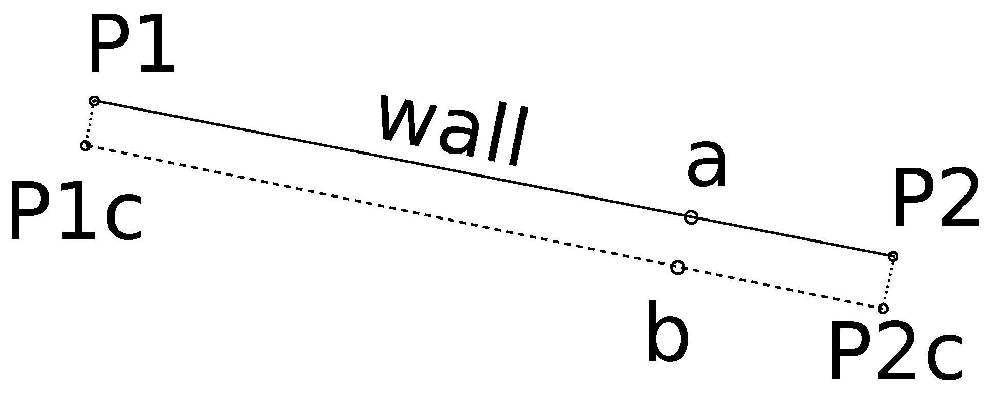
Müller-Fembeck presents a situation where currently no legally clean solution exists [16]. A wall, which was surveyed in the 1970s, marks a boundary. At that time, a deviation of 20 cm was acceptable. What if a surveyor needs to define a point on this wall today, e.g., as a boundary point separating two parcels on the same side of the wall? The limited accuracy of the original survey could lead to the situation shown in Figure 1.

Figure 1. Visualisation of the problem discussed by [16].

The solid line represents the surface of the wall, which should coincide with the boundary line. The distance between the wall points (P1 and P2) and the positions determined by the coordinates (P1c and P2c) is almost 20 cm. They are treated as equal, i.e., by law, the wall is identical to the boundary line. In version a, the point is marked and surveyed directly at the wall. This results in a bent boundary line (P1c–a–P2c). In version b, the new boundary point is calculated mathematically, but when staking it out, the position that has to be marked is not on the boundary in the field.

3. GNSS Positioning and Transformations

3.1. Reference Frames

The representation of positions in a reference system requires the definition of a coordinate system. There are local and global definitions, and the latter ones are relevant, for example, when using GNSS. The currently used global reference frame is the International Terrestrial Reference System (ITRS). Due to continental drift and other influences, the Eurasian plate moves in the range of centimetres per year [18]. Thus, the global reference system ITRS is not suitable for many applications in the European context. ETRS89 is the European realisation of the datum definition. The currently valid reference frame in Austria as a realisation of the ETRS89 is EUREF Austria 2002 [14,19,20].

The Austrian geodetic reference system is the MGI system defined in 1892. The Bessel ellipsoid from 1841 serves as a reference surface. The Gauss–Krüger projection (transversal cylindrical projection) provides the mapping to the planar coordinate system [5,10,14,21]. The control points realise the national system MGI and serve as a starting point for the surveys in the national coordinate system. The stabilisation of the triangulation points is primarily based on granite stones with underground backup. This ensures the permanent representation of the national coordinate system. Other types of stabilisation, such as iron tubes or metal plates, are also common in the case of lower-level control points. § 1 VermV stipulates the precision in the determination of control points using a two-dimensional simple mean point-position accuracy of 2 cm for triangulation points and 3 cm for the lover-level control points. This is determined by adjustment of measurements in MGI. However, the law acknowledges that this validity is limited by systematic effects due to ground movements, network stresses, or changes in stabilisation [10,13,14,22,23].

3.2. GNSS Positioning and RTK Implementation in Austria

The position of a GNSS receiver is determined by the time-of-flight measurement to at least four satellites. By differential measurement and the use of reference stations with known coordinates, RTK measurements can achieve accuracy better than 1 cm in position [24]. With a receiver close to the reference station, it can be assumed that the position errors are approximately the same as those directly at the reference station, due to the described error influences, and thus, the calculated correction data can also be transferred to the moving receiver [20].

High-precision positioning using satellite navigation systems for the entire territory of Austria requires a nationwide infrastructure of reference stations. The Austrian Positioning Service (APOS) is operated by the BEV and currently comprises 36 permanent GNSS reference stations (average distance of 50 km) throughout Austria, as well as additional stations in neighbouring countries for cross-border networking. Since 2019, APOS, as a multi-GNSS service, has used the signals of GPS, GLONASS, and GALILEO systems, and thus provides a real-time service for homogeneous 3D coordinates in the ETRS89 system. With an availability of 99.5% (24 h a day, 7 days a week) and almost 1500 customers (as of October 2021), the Austrian service is reliable and in-demand. The BEV offers APOS Real Time in various data formats, and mount points for users of RTCM-capable GNSS receivers [25,26].

When using APOS, it is possible to choose between the two concepts, namely Virtual Reference Station (VRS) and Master-Auxiliary Concept (MAC), for the network RTK solution. The service provides its own mount points for this purpose, via which the correction data for the respective method can be obtained. The basic principle follows the determination of correction values of the satellite signals at a coordinate-known reference station, and the calculation and transmission of the corrections of a moving receiver in the vicinity of the reference station. By using a network of reference stations, the corrections can be determined more accurately and the data can be calculated in a networked manner at a master station. Therefore, this case is referred to as network RTK [14,20].

In the VRS concept, a virtual reference station is generated in the immediate vicinity of the moving receiver, with virtual measurement data and correction data based on calculations in the computing station, derived from the measurements in the reference station network. In this process, the receiver sends its approximated position to the processing centre and receives the corresponding correction data via a wireless data link. By attaching the correction data to the receiver’s measurements, the error effects of the inaccurate satellite orbit data, as well as the propagation delay of the signals through the troposphere and ionosphere, are corrected, enabling centimetre-accurate positioning [14,27].

The second RTK variant of point determination that is possible with APOS is the MAC. In contrast to VRS, where most of the evaluation takes place externally in the data centre, here, the calculation takes place directly at the moving receiver. First, the user sends their approximate position to the APOS centre and receives the raw GNSS data measured there from the nearest reference station (master). From further reference stations (auxiliary) included in this concept, defined by a fixed number or a selected radius, the receiver receives coordinate and correction differences relative to the master station. These data are then used on the receiver side to calculate the position. The advantage of this method is the traceability of the position determination, since the baseline evaluation is not completed with respect to a virtual reference station, but to a physically existing station with fixed coordinates [14,20,27].

4. Methods to Stake Out Points within the Legal Boundary Cadastre

Current surveying regulations demand that boundary markers in the real world are determined and compared with the markers shown in the original surveying document. In addition, the unchanged positions of the boundary points need to be checked, considering the tolerances at the time of the last survey. Boundary markers must be physically identical (§5(2) VermV) and undamaged. This excludes the use of a lying or oblique boundary marker. Boundary points from the legal boundary cadastre are reconstructed from their coordinates if the markers are missing. The coordinates of the boundary points refer to the (inhomogeneous) geodetic reference system (MGI). The Austrian Survey Act defines the closest control points as being in the survey area and ensuring a homogeneous neighbourhood relationship in terms of accuracy theory. This allows for the elimination of a control point that lies within the survey area, but shows large tensions when compared to the surrounding points. In case of terrestrial measurement, at least two control points must be used, and in case of GNSS measurement, there must be at least four control points. The legal requirement is a maximum deviation of 5 cm between a new determination of boundary points and their original coordinates.

GNSS measurements have become standard in cadastral surveying due to their cost and time benefits. Since 2010, it has been legally possible to connect to MGI purely with GNSS. However, there were no specifications for the number of control points used, for the maximum values of the residual gaps, or for the maximum scale factor until 2016. All surveys conducted before 2010 rely on datum definition from terrestrial measurements only. Inhomogeneities in the control point network can cause significant deviations between coordinates determined by terrestrial surveys and GNSS surveys. In addition, control points suitable for a terrestrial survey are not necessarily usable with GNSS, e.g., due to obstructions. This can lead to different configurations of control points for the datum determination.

MGI suffers from historical surveying problems. The network was determined by terrestrial triangulation with a single distance measurement in each of the plane coordinate systems (base length 2.5–10 km). Due to missing calculation resources in the 19th century, the network was never fully adjusted before using it as a basis for cadastral surveys. The attempt to adopt photogrammetry in the 1970s failed to achieve the required quality with the available budget. A resurvey of control points with GNSS revealed a nationwide inhomogeneity of up to 1.5 m, with a much better relative accuracy [25]. Distortion vectors can be derived from the control point database of the BEV. The BEV provides an Austrian-wide NTv2-based grid solution [28], the GIS GRID, to eliminate the distortions and transform between ETRS89 and MGI. However, the quality of this grid was not intended for cadastral applications and is not fit for purpose in this context [29], since the lower-level control points were not used for the parameter estimation. This prevents the use of this approach, and the transformation parameters have to be determined separately for each local survey.

Two situations need to be distinguished:

• Reconstruction in an area with a homogeneous control point network;
• Reconstruction in an area with a distorted control point network.

4.1. Homogeneous Control Point Network (M1)

A (sufficiently) homogeneous control point requires that positioning based on more than four nearest control points leads to a precision value of the boundary points of less than 2 cm ($1\sigma$) and a maximum residual of 5 cm. In such a situation, the coordinates determined by GNSS or terrestrial surveys will not differ significantly, and either solution is suitable for the reconstruction.

The transformation needed due to regulations is a 2D Helmert transformation, which is a conformal transformation [30] with at least four identical points (points where the coordinates are known in both coordinate systems). The geometrical configuration of the control points must guarantee good coverage of the surveyed cadastral area and consider the neighbourhood relations in the control point network [23].

4.2. Distorted Control Point Network

In case of a distorted control point network, a 2D Helmert transformation is also used to reconstruct point positions (coordinates). However, the scale can be much larger than in the homogeneous situation. § 1 (17) VermV regulates that the scale must not exceed a change of 100 ppm (parts per million). The transformation parameters are determined based on identical points. Identical points are boundary points that are shown in the survey document and are clearly identified and still located in their original position in reality. Proving this unchanged position is usually achieved by visual inspection and distance measures to other identified points. MGI coordinates have to be available for the identical points, but they do not need to be in the legal boundary cadastre. The problem with this solution is that the control points receive new coordinates. Since their coordinates are fixed, the residuals need to be eliminated. This can either be solved by local distribution of the residuals or by the use of homogeneous vectors.

4.2.1. Transformation Based on Local Distribution of the Residuals (M2)

An inverse distance-weighted interpolation (IDW) provides one method to eliminate the residuals [31]. For a new point, the coordinate correction is determined via the known residuals of the surrounding control points from the transformation. The shorter the distance between the new point and control point, the greater the influence of the residual of the respective control point on the correction of the new point. The calculation must be carried out individually for the Y and X coordinates of each point.

The advantage of this method is the simplicity of calculation. It does not assume much, except for a continuous decrease in correlation with distance. However, as with other, more complex approaches, it cannot cope well with breaks in the spatial relation. Older surveys creating the parcel structure for a larger area might be consistent in geometry. However, the survey might be based on only three control points and may ignore control points that do not fit these points. Surveys based on these ignored points will cause break lines in the transformation parameters along the border of the surveying areas. These break lines may cause residuals of 10 or 15 cm, and cannot be handled well by methods such as IDW or similar approaches such as the membrane method [32]. In general, approaches such as rubber-sheeting [33] will fail when parts of the cadastral boundaries or the control network move, and the user will not receive a warning.

4.2.2. Transformation Based on Homogeneous Vectors (M3)

It is possible to determine homogeneous coordinates for all Austrian control points by resurveying the points with GNSS. Unfortunately, these coordinates cannot be used as a reference system because positions determined from them do not match positions determined earlier, in the distorted, old system. This would seriously impact the use of all historical data. The difference between the coordinates of a point in the homogeneous and the old system is called a homogeneous vector, and simplifies the transformation between ETRS89 and MGI [14]. The components of these homogeneous vectors are then used as input for IDW.

4.3. Comparison of Methods on Three Examples

The methods discussed were tested for their practical suitability by means of three examples. The examples were taken from the daily office routine of the company geolanz ZT-GmbH and were selected as representative examples of surveys in the legal boundary cadastre under different conditions. Supplementary measurements were taken to check the original document. Calculations and plots were performed with rmGEO, GeoMapper, and rmMap software by rmDATA. The calculation of IDW was implemented in Microsoft Excel. For evaluation and comparison of the calculated values, the interpolated positions are compared with the coordinates according to the cadastre.

4.3.1. Case Study Gallneukirchen

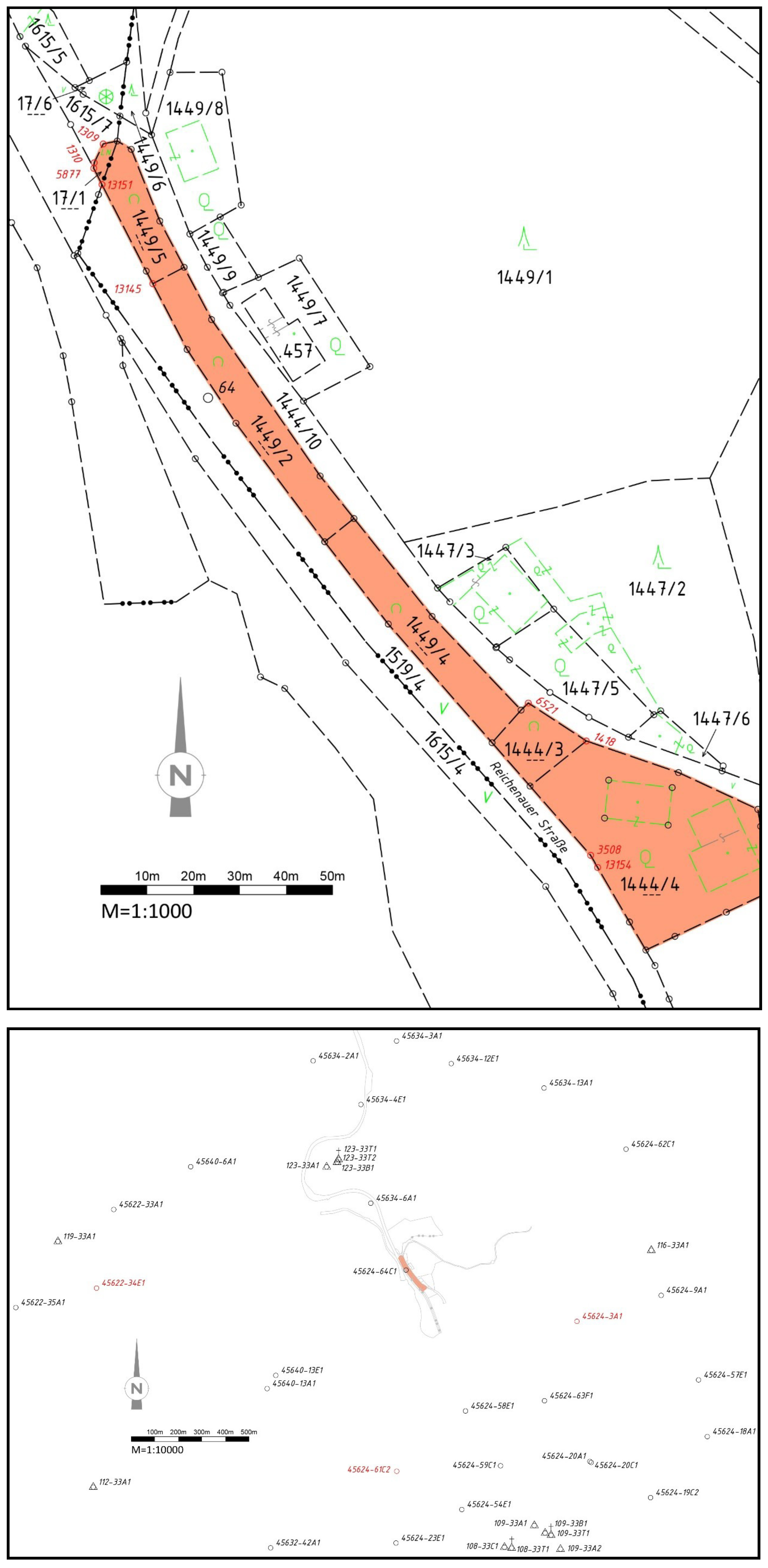
The boundaries of parcels 17/1 (in Oberndorf), 1444/3, 1444/4, 1449/2, 1449/4, and 1449/5 (in Gallneukirchen) should be made visible in the real world (compare Figure 2 top). All parcels were converted into the legal boundary cadastre in 2001. During the survey, nine boundary marks, which are identical with the original document, were found in the real world, but show a shift when compared to the results of georeferencing according to the current surveying regulations.

Figure 2. Cadastral map showing the affected parcels (top) and overview of the control point network (bottom). The control points marked in red do exist but are suspended from use (data: BEV).

The bottom of Figure 2 shows the control point network in the area. Control points 45634-6A1 and 45634-34E1 were originally used to connect it to the cadastral survey. The originally used control point 45634-34E1 was lost in 2001. Point 45624-64C1 (approximately 20 cm from the original point) is used for the further calculations in this example. The effects of network distortions on this point are assumed to correspond to those of the lost point.

The overview of the distortion of the control point network published by the BEV (Figure 3) shows that the distortions of 45634-6A1 (determined by photogrammetry) and 45624-64C1 (determined by terrestrial survey), represented by arrows, point in different directions. The magnitude of the distortion is in the decimetre range, although both points should have a precision of a few centimetres. However, since the point definition was achieved independently, the deviations might have added up, and the magnitude of distortion shows that the requested precision was not reached. Figure 3 also clearly shows a large variation in the direction of the distortion. Using these two points to determine transformation parameters resulted in a small rotation of 1.3 arcseconds and residual gaps of almost 11 cm (compare Table 1). This is a further indication of an inconsistent control point network. The residual gaps exceed the maximum value of 5 cm required by surveying laws. However, there is often a lack of alternatives for reconstructing the datum definition of a surveying document.

Figure 3. Distortion of the control points in Gallneukirchen. The red arrows show the direction and amount of large distortions (data: BEV).

Table 1. Residuals of control points after conformal transformation.

Point	Residual Y [cm]	Residual X [cm]
116-33A1	−4.8	−1.7
123-33A1	−4.4	0.2
45622-33A1	−2.1	−3.0
45622-34E1	5.5	4.3
45624-3A1	9.8	−1.2
45624-58E1	3.1	−1.7
45624-59C1	−5.8	−8.8
45624-62C1	−1.8	10.5
45624-63F1	−3.6	1.5
45624-64C1	−3.5	−4.2
45624-9A1	2.2	2.9
45634-12E1	−0.1	−2.8
45634-13A1	1.2	−4.2
45634-4E1	−2.5	5.7
45634-6A1	5.7	0.9
45640-13E1	1.2	−3.1
45640-6A1	4.6	4.6

The residuals of points 45624-64C1 and 45634-6A1 differ by 9.2 cm in the y-direction and by 5.1 cm in the x-direction. The distortion between these two neighbouring control points (distance approximately 320 m) is obvious.

All nine boundary marks of the survey that were found in the real world were re-measured according to surveying regulations. Boundary points 3508, 13145, and 13151 had to be eliminated, because the residuals exceeded the 5 cm per coordinate acceptable to assume an identical point position. The elimination was performed iteratively, and one point was eliminated per iteration until the residuals of the remaining points were below the limit. The remaining point coordinates are assumed to be homogeneous, and can be used as tie points for a local transformation. Table 2 shows the residuals for the boundary points of the first iteration.

Table 2. Results of the different methods: M1 (local transformation by 2D Helmert transformation), M2 (IDW based on residuals), and M3 (IDW based on homogeneous vectors).

Point	M1		M2		M3		Comment
	Y [cm]	X [cm]	Y [cm]	X [cm]	Y [cm]	X [cm]
1309	−5.6	5.3	−7.1	2.8	−7.4	2.2
1310	−6.1	2.2	−7.7	−0.4	−7.9	−0.9
1418	−7.6	0.5	−10.8	−1.5	−11.1	−2.1
3508	−5.5	7.7	−6.9	5.8	−7.2	5.2	residuals > 5 cm
5877	−5.0	0.5	−6.5	−2.1	−6.8	−2.8
6521	−6.6	−3.0	−8.2	−5.2	−8.4	−5.8
13145	−15.3	−1.2	−16.3	−4.1	−16.6	−4.7	residuals > 5 cm
13151	−11.6	3.2	−13.2	0.6	−13.5	0.0	residuals > 5 cm
13154	−8.4	0.3	−9.8	−1.6	−10.0	−2.2

In this example, the boundary points satisfy the legal requirements of a misplacement of less than 10 cm at least for several points. Thus, M1 is a suitable procedure. The other methods do not significantly improve the misplacement.

4.3.2. Case Study Gramastetten

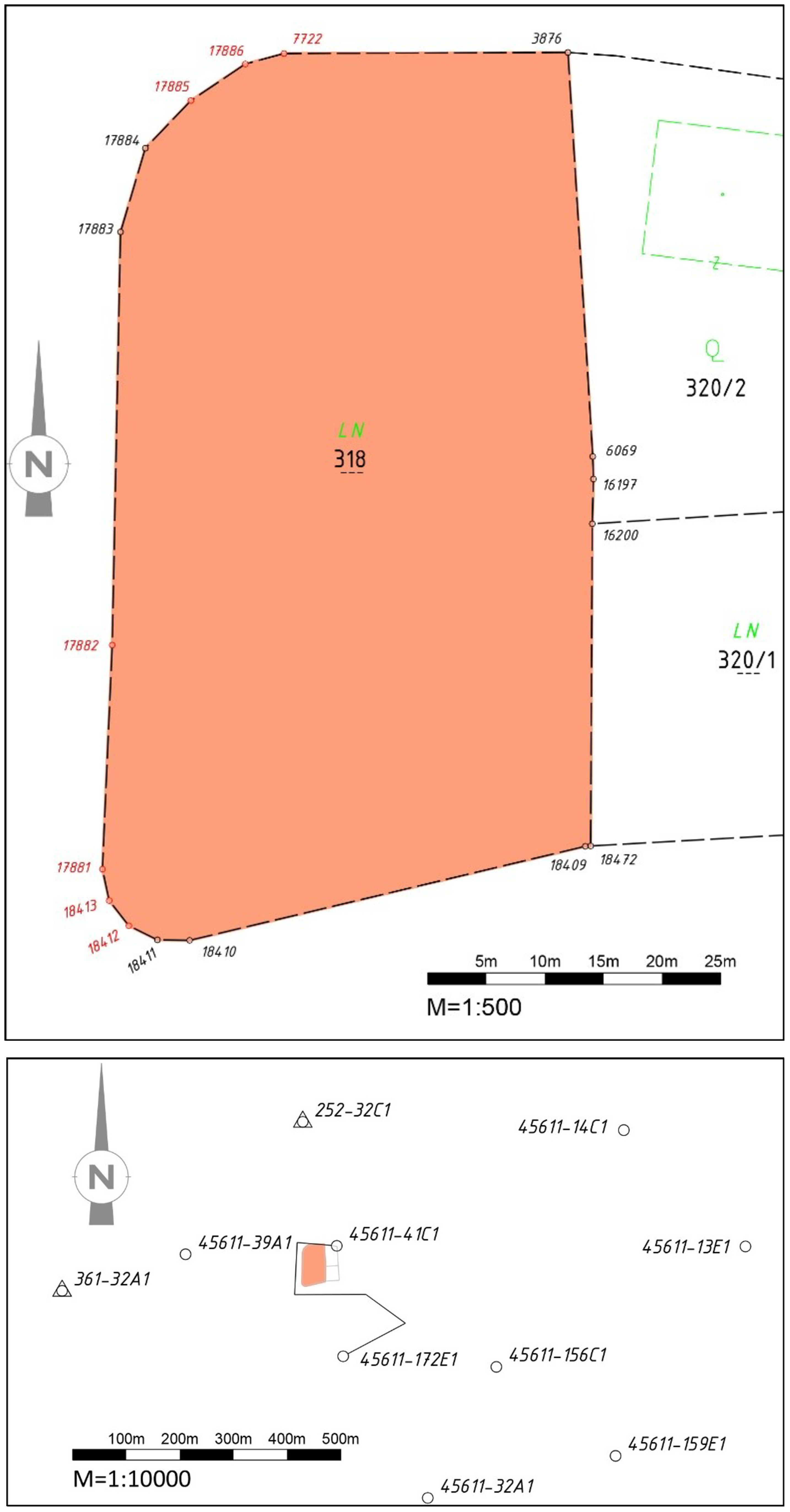
The task here was the parcellation of large parcel number 318 (Figure 4 top), which was transferred to the legal boundary cadastre in 2006. The bottom of Figure 4 shows the available control points in the area.

Figure 4. Cadastral maps showing the affected parcel. Boundary marks that have been found in the real world are plotted in red (top). Overview of the control point network including the traverse used to survey the parcel (bottom).

The survey from 2006 used photogrammetrically determined control points (45611-41C1 and 45611-172E1). The church in the centre of the figure (252-32T1) was used for orientation, although it is too close to the measurement area so aiming is difficult. During the new GNSS survey of the existing boundary markers, a systematic positional deviation of the boundary points in the Y- and in X-directions was detected when using GNSS. The control points still exist, but the polygon points created for the survey are lost. Table 3 lists the control points used and the associated residuals from the GNSS transformation with a scale of 1.

Table 3. Residuals of control points after conformal transformation.

Point	Residual Y [cm]	Residual X [cm]
252-32C1	1.3	−0.1
361-32A1	−1.6	−2.1
45611-13E1	−2.7	−5.7
45611-14C1	−1.6	−2.4
45611-156C1	4.2	1.1
45611-159E1	−0.7	0.9
45611-172E1	8.4	6.9
45611-32A1	−2.9	3.0
45611-39A1	−0.2	−7.9
45611-41C1	−4.3	6.4

The control points 45611-172E1 and 45611-41C1 have relative residuals (the difference between their respective residuals) of 12.7 cm in the Y-direction and 0.5 cm in the X-direction. The distance between them is only 206 m, resulting in a scale factor of 617 ppm, exceeding the limit of 100 ppm. Possible reasons for this include problems with the original determination of the coordinates or soil movement. The problem was not present in the 2006 survey. Two aspects seem plausible: (i) the traverse used in 2006 has an s-shape—the limits for the traverse tolerance use the length of the traverse and this could have masked the stress—or (ii) the land movement started to accelerate after 2006. Overall, the control point network in the area is distorted. 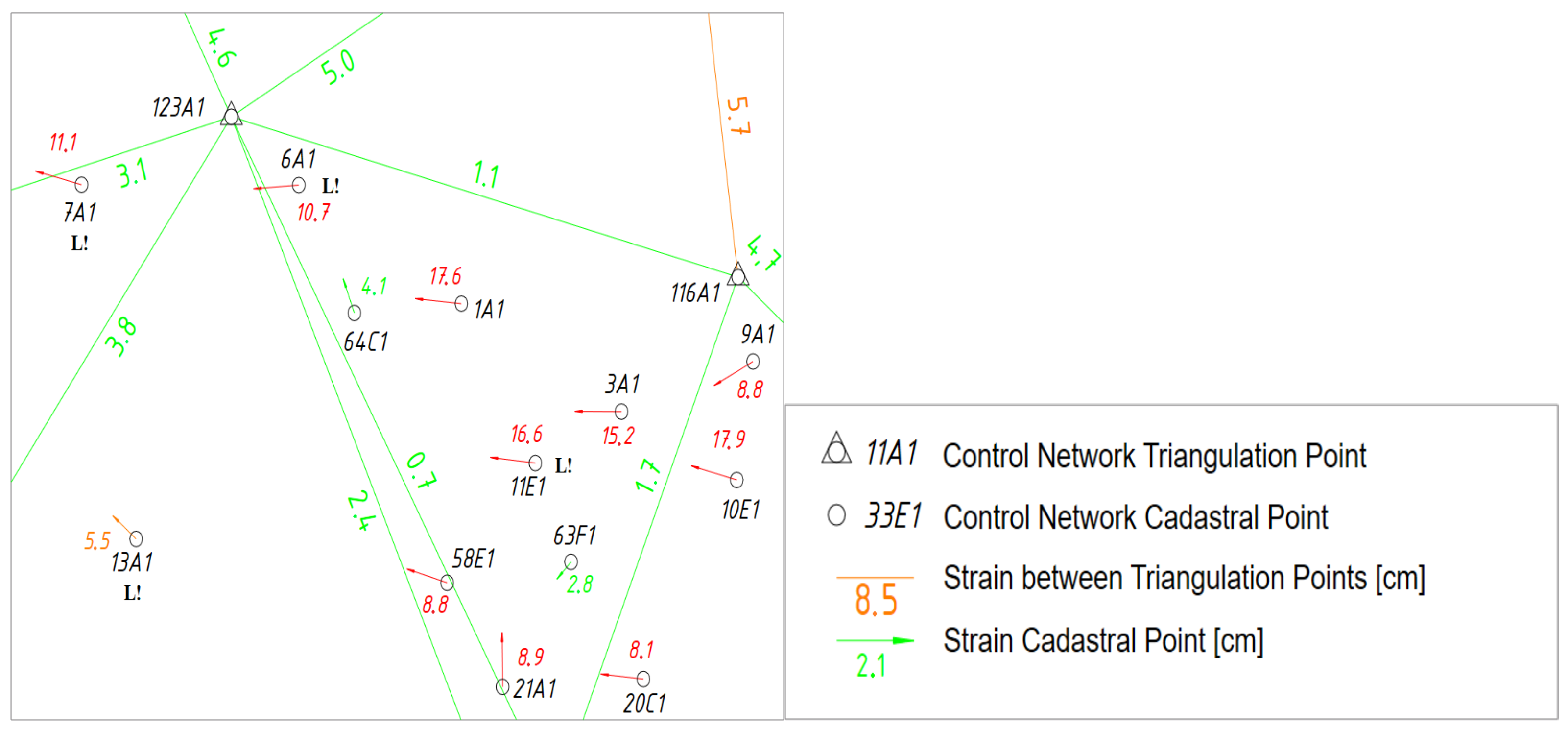Figure 5 shows the strains of the homogeneous vectors of the control points. The colour, size, and direction of the arrows provide information about the homogeneity of the individual control points. The annotation “L!” identifies control points determined by aerial photogrammetry in the 1970s. The strains in the network are clearly visible because there is no visible systematic in the direction of the distortion errors. In particular, the large arrows (in red) point in varying directions.

Figure 5. Distortion of the control points in Gramastetten. The red arrows show the direction and amount of distortion (data: BEV).

A 2D Helmert transformation based on found boundary markers from the original survey was possible. The requirements of having at least three identical points and a scale smaller than 100 ppm are met. The rotation of approximately 543cc is an indication that the orientation of the original survey was insufficiently stabilised due to the close church tower used for the orientation. The resulting residuals are less than 2 cm. This confirms the quality of the internal geometry of the original survey. However, connection to the control point network is difficult. Table 4 shows the results of different approaches if using the control points from the original survey. The accuracy does not fulfil the legal requirements. The residuals are again only a few centimetres. The absolute deviations of the calculated coordinates, however, are up 8 cm, which exceeds the legal limits of 5 cm. The distortion of the control points 45611-41C1 and 45611-172E1 is likely the reason for these deviations. Table 4 summarises the results. Table 5 shows the results when using all control points within 500 m from the parcel.

Table 4. Results of the different methods using the two originally used control points: M1 (local transformation by 2D Helmert transformation), M2 (IDW based on residuals), and M3 (IDW based on homogeneous vectors).

Point	M1		M2		M3
	Y [cm]	X [cm]	Y [cm]	X [cm]	Y [cm]	X [cm]
7722	4.1	−3.9	1.4	1.0	1.2	0.5
17881	10.3	−4.7	8.7	0.4	8.4	0.0
17882	7.9	−5.5	5.9	−0.4	5.6	−0.9
17885	2.5	−4.0	0.1	0.9	0.0	0.5
17886	3.2	−3.6	0.6	1.3	0.5	0.8
18412	9.4	−6.0	7.7	−1.0	7.4	−1.4
18413	8.2	−4.0	6.7	1.1	6.3	0.7

Table 5. Results of the different methods using all control points within 500 m around parcel 318: M1 (local transformation by 2D Helmert transformation already shown in Table 4), M2 (IDW based on residuals), and M3 (IDW based on homogeneous vectors).

Point	M1		M2		M3
	Y [cm]	X [cm]	Y [cm]	X [cm]	Y [cm]	X [cm]
7722	4.1	−3.9	1.8	−1.2	1.8	−1.8
17881	10.3	−4.7	8.5	−2.8	8.3	−3.1
17882	7.9	−5.5	5.9	−3.2	5.8	−3.8
17885	2.5	−4.0	0.5	−1.5	0.4	−2.0
17886	3.2	−3.6	1.0	−1.0	1.0	−1.7
18412	9.4	−6.0	7.5	−3.9	7.3	−4.5
18413	8.2	−4.0	6.4	−1.8	6.2	−2.4

Due to the strains in the control point network, a conformal transformation is not feasible. It is recommended to use the control points from the original survey to determine the transformation parameters. Using more points does not improve the accuracy of transformation in this situation.

4.3.3. Case Study Lachstadt

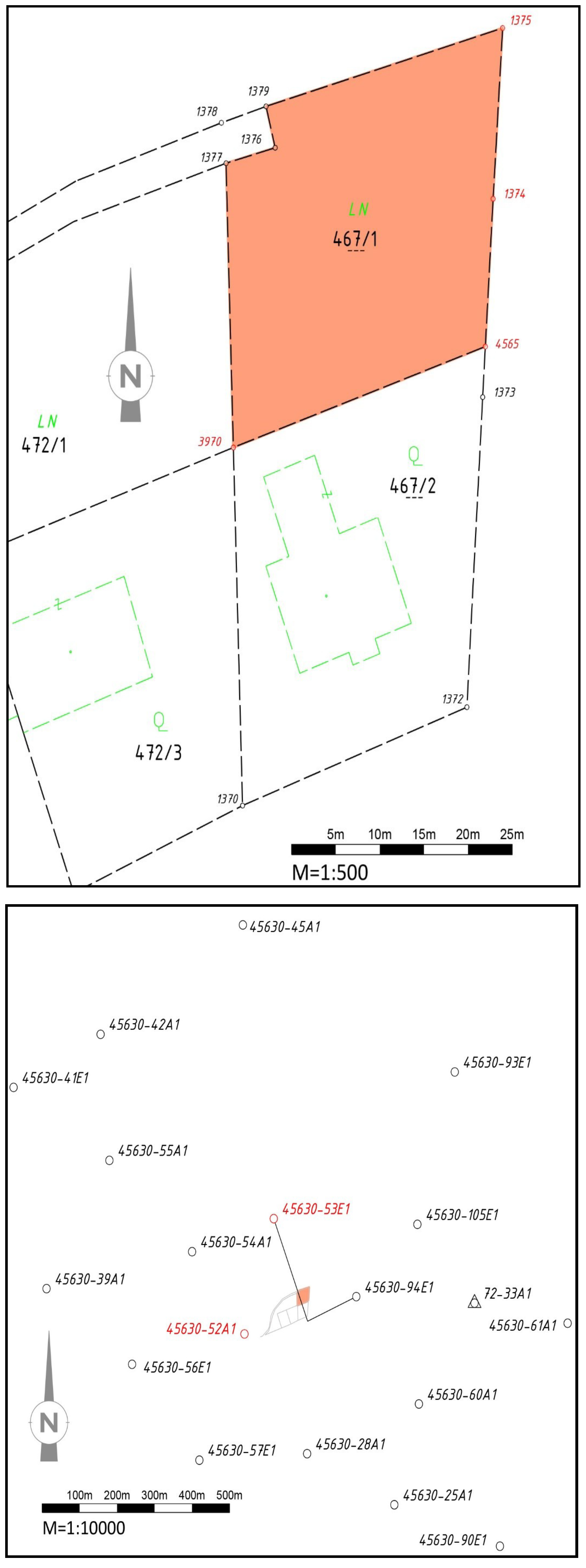
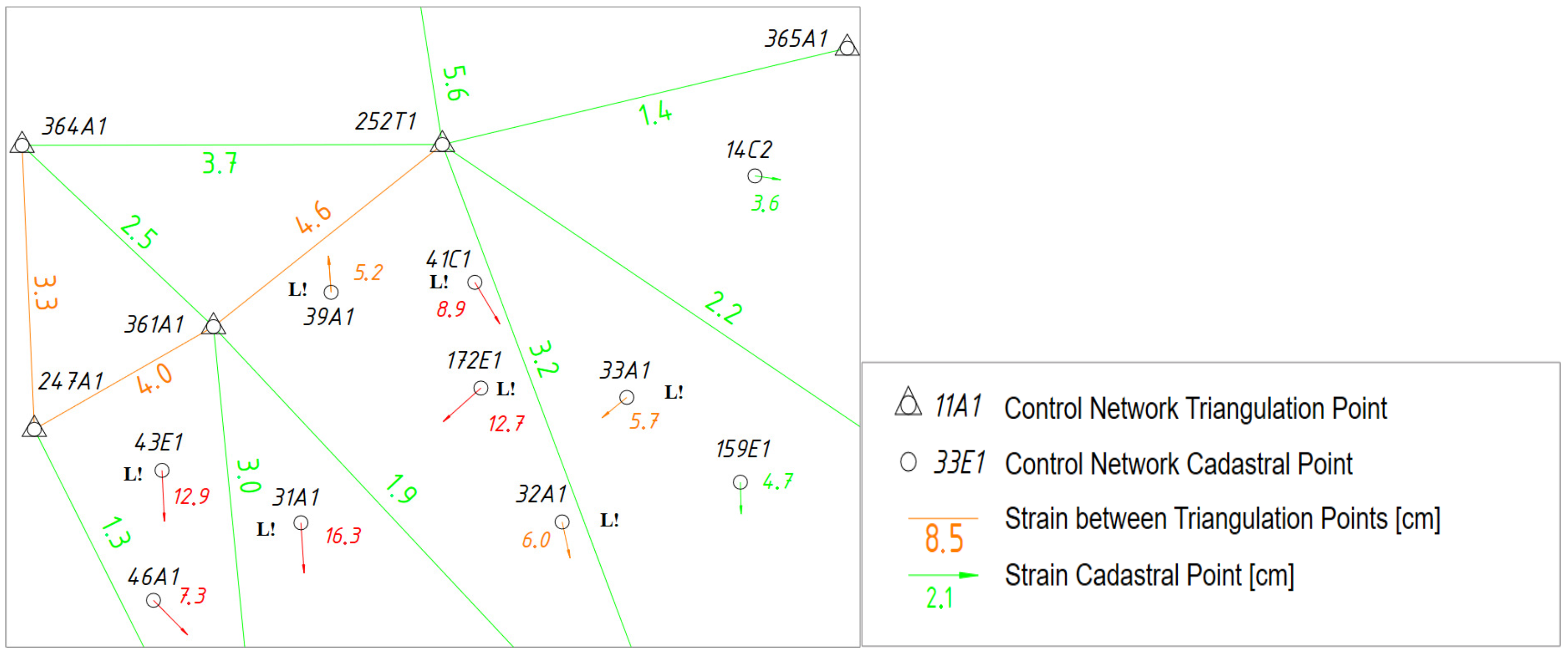
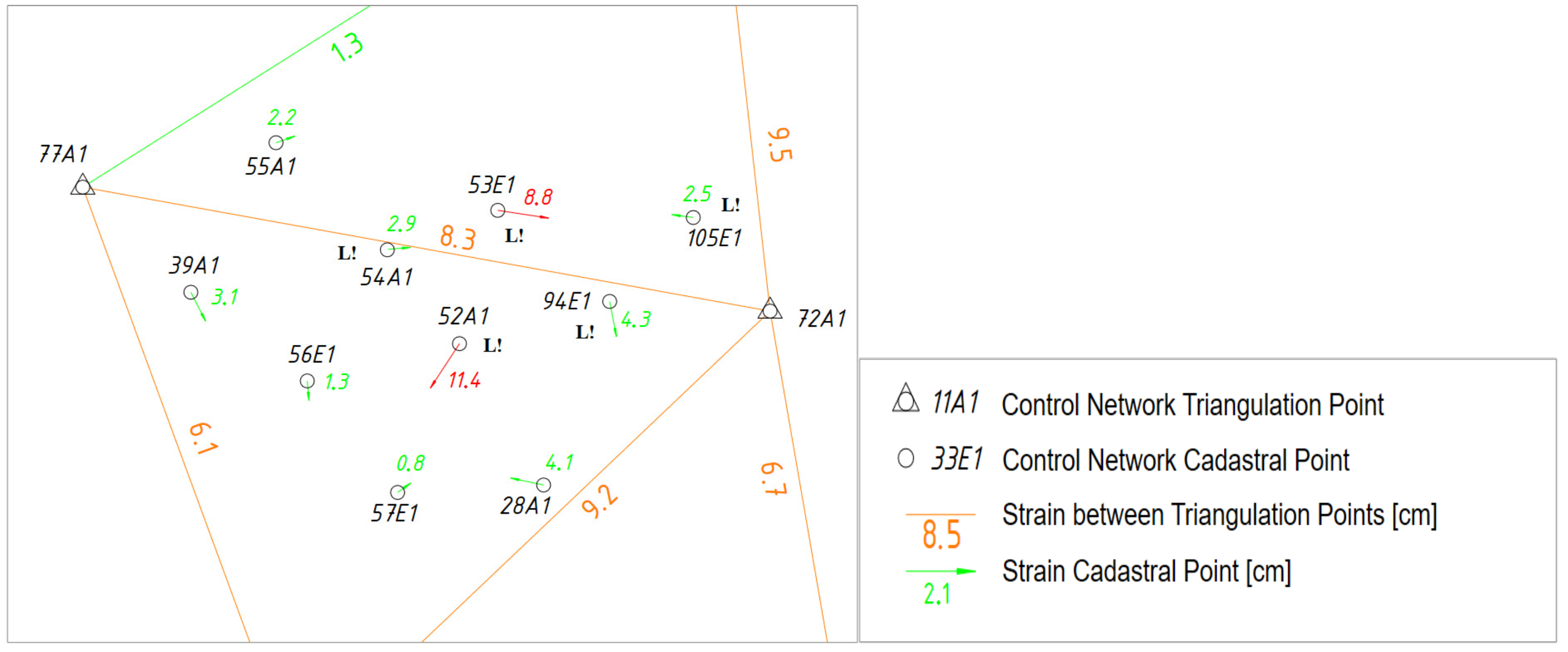
The boundary points of parcel 467/1 (cadastral municipality Lachstadt) were to be staked out. Four boundary markings identical to the survey from 1994 were found, and were used for the local transformation. An extract of the digital cadastral map with boundary points that still physically exist is shown at the top of Figure 6. The control points around the measurement area were determined mostly by photogrammetry. Therefore, the strains in the control point network (Figure 7) do not follow any systematic pattern. The bottom of Figure 6 shows the control point network in the area. The point density is high, which is a result of the photogrammetric measurements. However, Figure 7 shows that the control points 45630-52A1 and 45630-53E1 do not fit the other control points close to the surveying area. Therefore, these two control points were suspended by the BEV and are no longer allowed to be used. The control points used for the original survey are shown in orange in Figure 7.

Figure 6. Cadastral maps showing the affected parcel. Boundary marks that have been found in the real world are plotted in red (top). Overview of the control point network including the traverse used to survey the parcel (bottom).

Figure 7. Distortion of the control points in Lachstadt. The red arrows show the direction and amount of distortion (data: BEV).

The 2D Helmert transformation using all control points results in an approximately homogeneous situation, which, at first glance, does not indicate strains in the control point network, since the closest control points 45630-52A1 and 45630-53E1 are no longer available and the more distant points fit the local network.

Only four identical boundary points still existed, but a 2D Helmert transformation was possible nevertheless. The result is a set of parameters with a scale of −612 ppm, which exceeds the 100 ppm limit. Although, given the limited survey area, this only causes small changes, the legal rules prohibit this solution. Thus, this method is not suitable. The two control points 45630-53E1 and 45630-94E1 have both been given official ETRS89 coordinates, even though the former control point is now no longer available from the BEV. Table 6 shows the interpolated values using the two control points that were connected to in the document of origin.

Table 6. Results of the different methods using the control points originally used: M1 (local transformation by 2D Helmert transformation), M2 (IDW based on residuals), and M3 (IDW based on homogeneous vectors).

Point	M1		M2		M3
	Y [cm]	X [cm]	Y [cm]	X [cm]	Y [cm]	X [cm]
1374	1.1	−7.8	−3.1	−9.5	−3.4	7.1
1375	−2.1	−0.9	−6.4	−2.5	−6.7	−0.2
3970	−1.3	−6.4	−5.7	−8.1	−6.0	−5.9
4565	0.0	−2.6	−4.0	−4.4	−4.3	−1.8

Table 7 shows the result if all control points in the area are used. In contrast to the interpolation with the control points of the origin document, the tendency of the displacement of the boundary points is visible when comparing the results from the residuals (M2) with those of the homogeneous vectors (M3).

Table 7. Results of the different methods using all control points within 500 m around parcel 467/1: M1 (local transformation by 2D Helmert transformation), M2 (IDW based on residuals), and M3 (IDW based on homogeneous vectors).

Point	M1		M2		M3
	Y [cm]	X [cm]	Y [cm]	X [cm]	Y [cm]	X [cm]
1374	1.1	−7.8	−6.5	−9.9	0.7	−6.6
1375	−2.1	−0.9	−9.8	−3.1	−2.7	0.2
3970	−1.3	−6.4	−8.7	−8.2	−1.3	−5.1
4564	0.0	−2.6	−7.5	−4.6	−0.2	−1.4

Since it is impossible to check the geometry of the old document in this example on the basis of the still existing boundary points, only the staking out of boundary points by local transformation is possible in this case. The control point network is nearly homogeneous after the elimination of the control points with the largest residuals.

5. Discussion

Due to the inhomogeneity of the Austrian coordinate system MGI, problems inevitably arise in the cadastre that cannot be solved with standardised approaches. The current surveying regulations provide a legal framework within which cadastral surveying must be carried out. Particularly, when connecting to the official control point network, local deviations must be taken into account and decisions on specific execution must be made on a case-by-case basis. The introduction of legally binding boundary point coordinates in the legal boundary cadastre made it possible to place parcel boundaries under the protection of trust. However, the decades following the introduction of the legal boundary cadastre showed that the control point network is not sufficiently accurate and stable in some parts of Austria. In these areas, the symbolic immutability of the boundary points and their coordinates creates a demanding geodetic challenge in everyday surveying. Staking out points according to their cadastral coordinates requires the analysis of local deviations, which requires legal and technical expertise.

In this paper, we analysed methods that could provide information on the displacement of boundary points in a distorted control point network. The examples showed that it is not possible to predict deviations from the results of local transformation. Rotation of the boundary points of a document remains undetected with the distance-weighted interpolation. The local 2D Helmert transformation yielded the best results for the cases of Gramastetten and Gallneukirchen, by complying with the legal requirements and providing geometries without distortions in areas with a stressed control point network.

The reconstruction of the connection with the control point network from an old survey document contains more uncertainty factors than simply the possible strains of the control points used. Unfortunately, not all surveying approaches adopted in the past meet today’s accuracy needs. Photogrammetrically determined control points in Austria may be an extreme case, but similar situations will occur in other countries too if the network exists for centuries. Control points are lost over time, e.g., due to construction work. On the other hand, control points may shift due to land movement, or have to be suspended because of increasing legal demands regarding the quality of the control point network. Even when the control points are perfectly fine, land movement may affect objects on the ground, including boundary marks, fences, walls, and houses. Technically, this results in the same situation. All of these influences impact cadastral work. It is often impossible to identify the reasons, but this might not be necessary. It is necessary, however, to develop strategies that can cope with these problems.

The approach of mathematically transferring the stresses in the control point network onto the boundary points is based on the assumption that the relation between calculated residuals or homogeneous vectors and the true coordinates of the boundary point is (at least nearly) linear with distance. It is also assumed that the shapes of the parcels are unchanged in the real world, and that the boundary point coordinates listed in the survey document were derived directly from the control points used. However, it is often the case that coordinates are taken from a previous survey, and small deviations between these coordinates and newly derived coordinates are accepted. This procedure is legally valid for boundary points that are not relevant for the survey.

Since there are no ideal conditions in the Austrian cadastre, no statement can be made about the exact amount or direction of the displacement with the help of the interpolation of residuals or homogeneous vectors. The assessment is only possible in a case-based manner, taking into account influences such as the configuration of the control point network and the deviation of the existing boundary marks from the coordinates according to the cadastre. These differences can only be determined by measurements in the area of interest. Similarly to the distance until which control points are usable for interpolation, the assessment of acceptable boundary configurations is also subjective, and eludes simple standard rules. Theoretically, a highly homogeneous control point network would be able to solve this problem. However, this is only true if the relative positions of control points and boundary points do not change, i.e., there is no local, horizontal land movement. This could be the case in flat parts of the world, but mountainous regions will always have such movements. However, the analysis also showed the need for a broader discussion on digital documentation of ownership boundaries in Austria. The contradictions between the intention of the legal boundary cadastre and the technical limitations due to the inhomogeneity of the reference frame, soil movements, and developments in measurement technology need to be thoroughly addressed to avoid constantly facing this kind of challenge.

A limitation of the paper is that the Austrian cadastre is purely 2D. Three-dimensional cadastres [34] have to deal with similar problems, but they expand the range of issues. Every land movement caused by gravitational forces affects both plane coordinates and height. However, there are also situations where land only moves vertically, e.g., due to post-glacial land rise or underground mining. This is not a problem for 2D systems, but it is for 3D systems. Finally, the parcels themselves may move if they are connected to a building sinking into the ground. The question of how to deal with these challenges needs to be addressed in the future.