Landslide Susceptibility Assessment Considering Spatial Agglomeration and Dispersion Characteristics: A Case Study of Bijie City in Guizhou Province, China

Abstract

Landslide susceptibility assessment serves as a critical scientific reference for geohazard control, land use, and sustainable development planning. The existing research has not fully considered the potential impact of the spatial agglomeration and dispersion of landslides on assessments. This issue may cause a systematic evaluation bias when the field investigation data are insufficient, which is common due to limited human resources. Accordingly, this paper proposes two novel strategies, including a clustering algorithm and a preprocessing method, for these two ignored features to strengthen assessments, especially in high-susceptibility regions. Multiple machine learning models are compared in a case study of the city of Bijie (Guizhou Province, China). Then we generate the optimal susceptibility map and conduct two experiments to test the validity of the proposed methods. The primary conclusions of this study are as follows: (1) random forest (RF) was superior to other algorithms in the recognition of high-susceptibility areas and the portrayal of local spatial features; (2) the susceptibility map incorporating spatial feature messages showed a noticeable improvement over the spatial distribution and gradual change of susceptibility, as well as the accurate delineation of critical hazardous areas and the interpretation of historical hazards; and (3) the spatial distribution feature had a significant positive effect on modeling, as the accuracy increased by 5% and 10% after including the spatial agglomeration and dispersion consideration in the RF model, respectively. The benefit of the agglomeration is concentrated in high-susceptibility areas, and our work provides insight to improve the assessment accuracy in these areas, which is critical to risk assessment and prevention activities.

1. Introduction

As the most common natural hazard in mountainous areas, landslides pose a serious threat to human life and property, the ecological environment, and regional economic development due to the difficulties brought by their complexity, group occurrence, suddenness, and uncertainty [1,2,3]. Recently, a more frequently occurring tendency of geohazards in China and an aggravation of risk in local regions has been noticed, and the national authority declared it would strengthen prevention (Ministry of Natural Resources, PRC, 2021 (http://www.gov.cn/zhengce/zhengceku/2021-03/19/content_5593875.htm (accessed on 16 April 2022)) in the context of global climate change and increased extreme precipitation events [4,5]. It has been evidenced that 7840 geohazards occurred nationwide in 2020, an increase of 26.8% over 2019, resulting in 139 deaths (missing), 58 injuries, and direct economic losses of CNY 5.02 billion (http://www.mnr.gov.cn/dt/ywbb/202101/t20210118_2598832.html (accessed on 16 April 2022)). Landslide susceptibility assessment provides a solid reference with its spatial perception of disaster occurrence probability [6,7]. A refined susceptibility map is critical and valuable to reasonably deploy disaster prevention resources and effectively mitigate the geohazard’s influence. Especially for developing countries with limited control experience and resources, the accurate recognition of high-susceptibility areas is urgently needed to guide hidden hazard surveys for the safety of people and assets.

In recent decades, relevant research on landslides has developed fruitful results in theory and modeling, which can be classified into physically or statistically based approaches according to the research perspective. Based on the mechanical analysis of slope stability, the physical model generally incorporates the physical mechanism of disaster occurrence and provides additional information on the hazard’s intensity, thus resulting in a higher prediction accuracy [8,9,10]. However, the intensive data requirement of a high-resolution, sophisticated parameter calibration and simulation process makes it suitable only for small-scale local studies, not to mention the physical condition variation of complex environments [10]. Thereby, feasible methods combined physical-based approaches with statistical techniques have emerged [11]. In contrast, a statistical model driven by historical data can quickly evaluate a credible result from a large spatial scale without many constraints [12], with commonly applied methods including the information quantity model [13], AHP [14], frequency ratio [15], weights of evidence, and the certainty factor [16]. Nevertheless, these traditional statistical methods are weak in revealing the complex nonlinear relationships between landslides and their influencing factors [17]. This flaw has given rise to artificial intelligence. As it overcomes the disadvantages of subjectivity in the process of index selection and weight determination, the machine learning method has gradually become an alternative to the traditional statistics one [18] and the commonly used methods include logistic regression (LR) [19], a support vector machine (SVM) [20], random forest (RF) [21], and artificial neural networks (ANNs) [22]. In addition, new hybrid methods integrating the machine learning method with the statistical method have been successfully used for landslide modeling [23]. Different conclusions have been drawn by researchers when choosing an optimal machine learning method for susceptibility assessment. For example, Cao et al. [18] pointed out that extreme gradient boosting (XGBoost) performed better than RF and the SVM in the geological hazard susceptibility of Jiuzhaigou. Pourghasemi and Rahmati [24] compared 10 advanced machine learning algorithms and found that RF worked best, and Chen et al. [25] reached the same conclusion in Long county in Northwest China, while some studies also stated that the SVM achieved an optimal result [26]. We believe that the marked differences in the natural environment and hazard-forming conditions of various study areas are the key reasons for the discrepancies in applicability of the same method. Different methods will have various performances with the same region and data input. Meanwhile, it is necessary to identify the most appropriate machine learning model for a specific study area [27].

In existing studies, the affecting factors usually contain the aspects of topography, geology, meteorology, hydrology, land cover, and human activity. The spatial distribution of landslides is usually incorporated in modeling as a sample rather than a parameter. Actually, landslides induced by either fault activity or heavy rainfall all exhibit a clustering feature, which means landslides are concentrated spatially and contribute to the distinctive aggregation phenomenon [10,28,29]. Certainly, this aggregation is not accidental; it is essentially formed by the compound conditions of internal environmental (such as geologic structure) and external effects (such as rainstorms or earthquakes) [30]. Therefore, the spatial agglomeration feature itself can reflect the degree of susceptibility and follow the pattern of greater aggregation with higher susceptibility. However, few studies have utilized this feature in modeling, thereby, to some extent, wasting valuable information that might enhance the assessment accuracy. Aiming at this problem, Wang et al. [31] proposed the idea of considering spatial heterogeneity through extracting the clustering result of landslides based on the agglomeration feature, and the resulting susceptibility map with a higher quality proved its feasibility. Other works incorporating heterogeneity information from the spatial distribution perspective had also achieved more reliable results [32,33], whereas another typical spatial feature in many studies, dispersion, expressed by the widely scattered pattern of hazards, interferes with the excavation of spatial heterogeneity [34]. This is because its randomness and contingency blur the relationships between the dependent (landslide occurrence) and independent (driving factors) variables among the various blocks of a study area. In return, the model accuracy will be reduced, and the susceptibility map may be systematically biased in local areas. Unfortunately, this issue has rarely been emphasized and handled within existing research. Kalantar et al. [35] found that the training sample selection had an effect on the accuracy of the susceptibility models and further emphasized the need for the investigation of random training data division. Thus, the spatial dispersion feature of samples may be a viable entry point for addressing this issue.

Moreover, there is a positive correlation between the spatial distribution of geohazards and the classification of susceptibility levels [36]. Based on the above analysis, we speculate that integrating the spatial agglomeration and dispersion feature will further polish an assessment’s effectiveness. On the other hand, much effort nowadays on susceptibility assessment has focused on computational enhancement of model algorithms while ignoring the available information from landslide data itself. Work dedicated to the application of spatial distribution information on this topic is still lacking. Therefore, this paper proposes two innovative methods including clustering attribute extraction and data preprocessing for these two characteristics, respectively. Taking Bijie in Guizhou province in China as an example, differentiated machine learning models are combined to map landslide susceptibility, and the assessment results are analyzed by multiple evaluation metrics. Meanwhile, supplementary experiments are discussed to verify the feasibility of the proposed methods and the possible systematic bias of overestimating less prone areas and underestimating more prone areas in a previous assessment. Our work provides insights on the accuracy and performance improvement of the susceptibility assessment model, especially in high-susceptibility areas, so as to offer more reliable technical supports for the preliminary planning, long-term monitoring, and management decisions of geohazards.

2. Materials and Methods

2.1. Study Area and Data

Bijie is located in the northwest of Guizhou Province, covering an area of 26,900 km² with a permanent population of 6.71 million people. Situated at the eastern edge of the North–South Seismic Belt of China, the terrain here is greatly undulating because of the high altitude in the west and low altitude in the east. The surface is strongly cut and dominated by karst topography and mountainous terrain, with many stratigraphic units and complex lithology in the area. It has a humid subtropical monsoon climate with abundant rainfall throughout the year, and there are 193 inland rivers longer than 10 km, contributing to a dense river network. Meanwhile, this area is rich in mineral resources, with 36.77 billion tons of coal reserves, ranked first in the province. The proven reserves of iron, sulfur, and phosphorus are also abundant, but the past extensive development had led to a relatively fragile ecological and geological environment [37]. These environmental conditions have jointly nurtured a situation of frequent landslides. Aside from economic development needs, the increasing human activities, including mining, urban infrastructure, and agricultural production, would further change the natural environment, contributing to more geohazards. For example, a high-position collapse occurred in Nayong county in Bijie on 28 August 2017 with 27 victims. One important factor inducing the event was the formation of goaf by long-term coal mining. Moreover, as the frequency and intensity of extreme precipitation have increased, being affected by global climate change, landslides induced by rainstorms or prolonged rainfall are increasing. A representative event was the large landslide in Dafang county in Bijie on 1 July 2016 due to continuous heavy rainfall, resulting in 23 victims. Therefore, we used Bijie as a representative area to perform landslide susceptibility assessment, and the relevant results can provide guidance for geohazard prevention and mitigation projects (Figure 1). Here, the online base map of Figure 1 and other geographic figures for spatial analysis in this paper are mapped by ArcMap (Version: 10.6; Copyright: Esri [38]).

The landslide data used in Figure 1 were obtained from “Spatial Distribution Data of Geological Hazard Points” of the Resource and Environment Science and Data Center (http://www.resdc.cn/data.aspx?DATAID=290 (accessed on 12 February 2022)), and relevant studies have corroborated its reliability [41]. This data set is a collection of historical inventories recorded cumulatively over several years in Guizhou, with a total of 1267 landslide events in Bijie.

2.2. Methodology

The proposed technical framework of this study is shown in Figure 2. Based on the observation of the landslide inventory of Bijie in Figure 1, we supposed that the typical spatial agglomeration and dispersion characteristics it presented brought implicit susceptibility information and noise interference, respectively (Figure 2a). First, by mining the clustering attribute implied in agglomeration, critical information that reflected the inter-regional heterogeneity was incorporated into the model (Figure 2b). Secondly, we filtered the original data based on the fishnet grid constructed and, in the meantime, generated the training set and test set (Figure 2c). Then, the clustering attribute, together with 14 other factors, constituted the affecting factors data set (Figure 2d). Once the data set successfully passed the collinearity analysis (Figure 2e), it would be input into multiple machine learning models. Thirdly, through comparing the prediction accuracy and the actual simulation effect of each model (Figure 2f), we identified the optimal method, mapped the landslide susceptibility, and analyzed the degree of susceptibility at the city and county levels (Figure 2g). Finally, two further experiments were designed to verify the advantages of our proposed methods and to quantify the impact of these two spatial features on susceptibility assessment (Figure 2h).

2.2.1. Machine Learning Models

Four representative and classic models were considered in the comparison analyses: LR, SVM, GBDT, and RF. LR is a common probabilistic nonlinear regression model for the binary classification problem, and it has been widely used in landslide susceptibility prediction [42]. The main idea of the SVM is to find a maximum-margin hyperplane which can correctly separate two classes of data points as much as possible and render these two classes as far as possible from the hyperplane [26]. Here, these two classes of points refer to true hazard and non-hazard points. GBDT is an iterative decision tree algorithm using the CART regression tree as the base classifier, and its basic idea is to build a strong classifier with multiple weak classifiers. It can accelerate the convergence to a locally or globally optimal solution while identifying complex nonlinear relationships [31]. Relying on the high accuracy and strong tolerance of outliers and noise, RF is currently recognized as one of the best machine learning models [43]. It is essentially an integrated algorithm consisting of substantial decision trees. The final classification result is determined by winning a majority vote or taking the mean value of the results derived from multiple differentiated trees. Twofold randomness in the sampling and feature selection of RF makes it hard to be over-fitted and enhances the model stability. A detailed introduction of these models is presented in the Supplementary Materials.

2.2.2. Accuracy Evaluation Indexes

Statistical methods and an ROC curve were adopted to evaluate the performance of the test sets. An objective comparison cannot be inferred with solely statistical metrics, and thus we used four indexes, including the $precision$, $recall$, $accuracy$, and $F1 score$. Here are their definitions:

$$Precision=TP/\left(TP+FP\right)$$

(1)

$$Recall=TP/\left(TP+FN\right)$$

(2)

$$Accuracy=\left(TP+TN\right)/\left(TP+FP+TN+FN\right)$$

(3)

$$F1 socre=2\ast Precision\ast Recall/(Precision+Recall)$$

(4)

where $TP$(true positive) is the number of correctly classified hazard points, $TN$ (true negative) is the number of correctly classified non-hazard points, $FP$ (false positive) is the number of misclassified non-hazard points, and $FN$ (false negative) is the number of misclassified hazard points.

A receiver operating characteristic (ROC) curve is a curve plotted with the true positive rate ($TPR$) as the vertical axis and false positive rate ($FPR$) as the horizontal axis at different classification thresholds. As an intuitive evaluation method, it can give objective and neutral advice. Another critical index is the area under the ROC curve (i.e., the AUC), ranging from 0 to 1. A larger area under the curve usually means a superior model:

$$TPR=TP/\left(TP+FN\right)$$

(5)

$$FPR=FP/\left(FP+TN\right)$$

(6)

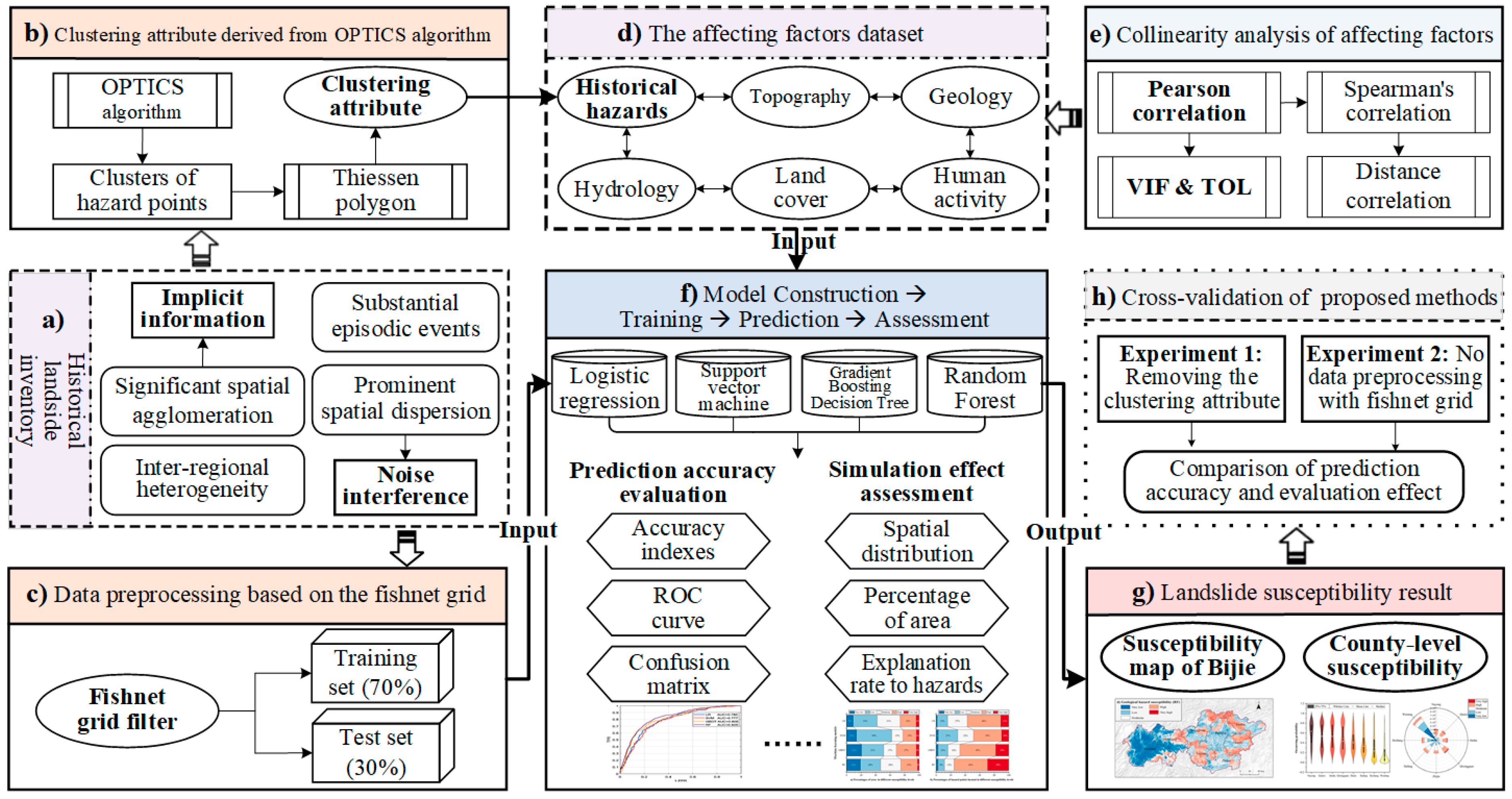
2.3. Strategies Considering the Spatial Characteristics of Landslides

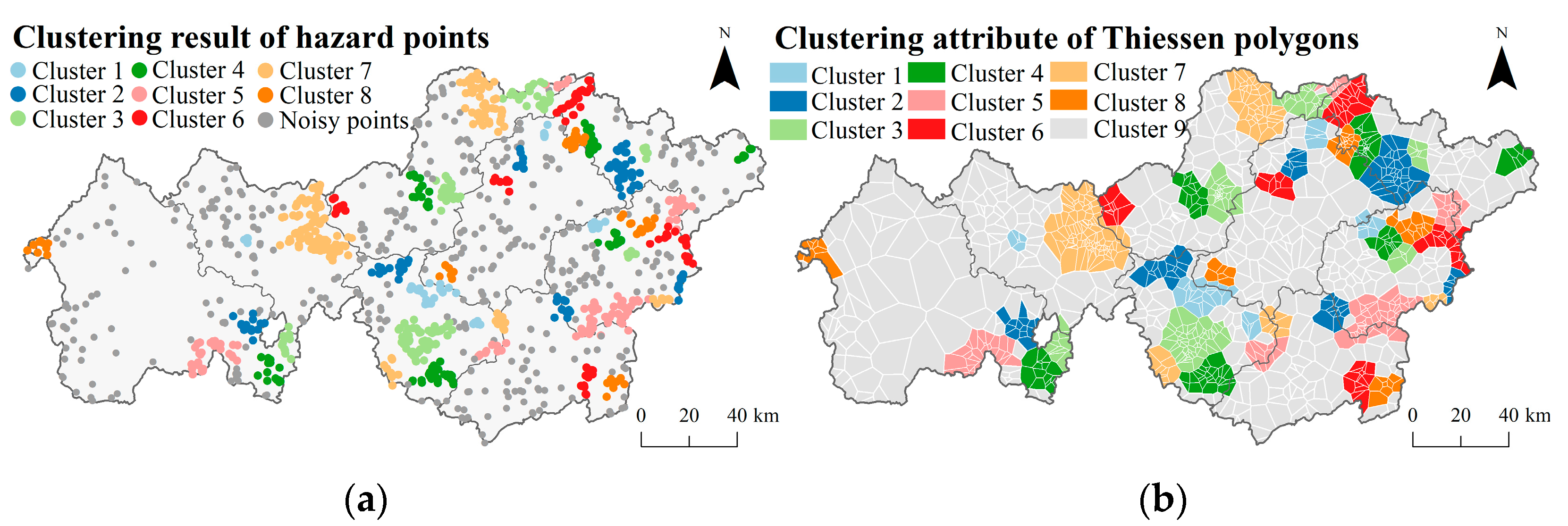
2.3.1. Clustering Attribute Derived from Spatial Agglomeration

As mentioned before, spatial agglomeration can be viewed as an intuitive phenomenon reflected by the long-term evolutionary law of landslides. An area with high agglomeration is more prone to hazards in terms of probability. Accordingly, the unused information it implies is valuable to susceptibility assessment. Here, we used the Ordering Points to Identify the Clustering Structure (OPTICS) algorithm to derive this potentially valuable information. It is a clustering algorithm for finding density-based clusters in spatial data. As an improved version of Density-Based Spatial Clustering of Applications with Noise (DBSCAN), it addresses the problem of detecting meaningful clusters in data of varying densities. Another advantage is there being no need to pre-set the number of clusters due to the automatic, ordered, and interactive cluster analysis [44].

The detailed introduction in the Supplementary Materials reveals that there are two main input parameters in the algorithm: the search distance of the neighborhood and the minimum number of points within it. The spatial scale of analysis is determined by the combination of these two parameters, and under different scales, the algorithm will find distinct clustering results. Therefore, in order to find the clustering attribute closest to the actual one, we tested the main combinations of these two parameters and identified the optimal one by comparing the model training accuracy of each machine learning algorithm (Figure 3). Then, the clustering results of the hazard points were assigned to the vector layer by using a Thiessen polygon (Figure 4) (see Supplementary Materials for the detailed procedure).

It is worth noting the property of the Thiessen polygons that each one of them contained only one hazard point, and the distance from any position of the Thiessen polygon to the hazard point was shorter than that of any other hazard point. This property ensured that each polygon was characterized by the same clustering attribute with the highest probability when the clustering results of the points were assigned to polygons [31]. Furthermore, it maintained similar hazard susceptibility within the same polygon block (composed of polygons with the same attributes), thus ensuring homogeneity in the same block and heterogeneity between different blocks.

Using a 10-fold cross validation training model, the test results indicated that the combination of 6 as the minimum number of points and 5 km as the search distance achieved the highest average accuracy of the 4 models at 76.8%, with RF being the best (up to 78.8%) (Figure 3). In addition, there existed some noteworthy patterns:

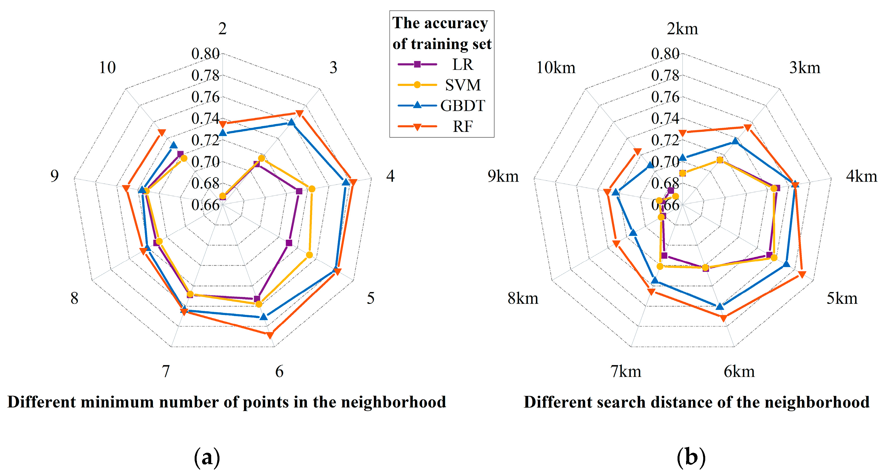
• The integrated algorithms such as GBDT and RF significantly outperformed the traditional machine learning algorithms such as LR and SVM in this study.
• No matter which parameter was taken as the independent variable, the accuracies of the models presented a linear trend of increasing first and then decreasing with the increase in the variable. This pattern implies the potential clustering feature in the spatial distribution of landslides, as we speculated. Meanwhile, the agglomeration reflected here represents the group-occurring characteristic of landslides.
• Demonstrated by the value and variation of the training accuracy, the models were more sensitive to the parameter of the search distance than the minimum number of points, which also manifested the spatial heterogeneity among different polygon blocks in the study area.

In summary, we recognize the optimal result shown in Figure 4 (the combination of 6 as the minimum number of points and 5 km as the search distance) as the final clustering attribute factor.

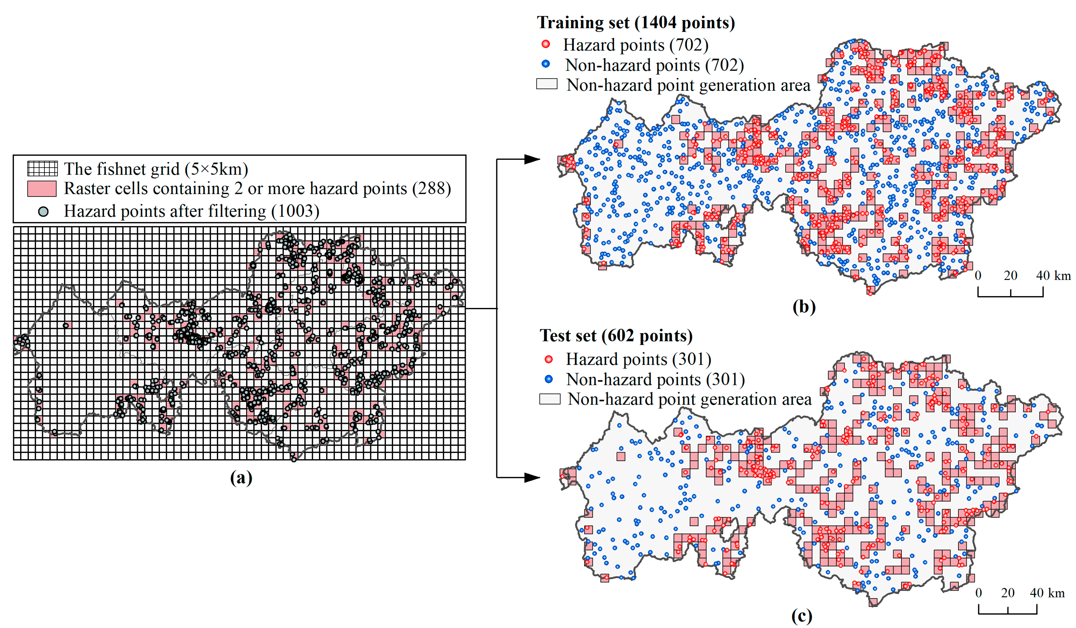
2.3.2. Training and Test Set Generated by the Fishnet Grid

The spatial dispersion areas with isolated hazard points are illustrated in Figure 1. Sparse hazards were usually due to the inherent stability of the slope, soil, and lithology. Limited accessibility to uninhabited areas and difficulty in sampling contributed to sparse hazard nodes as well. Subsequently, these sparse locations may have introduced inherent subjectivity and uncertainty to the data set, concealed the group-occurring feature, and then induced regional assessment bias. From an algorithm perspective, isolated hazards could not consistently reflect the relationship between the affecting factors and landslide occurrence but diluted the relationship between the affecting factors and susceptibility; that is to say, the dispersion feature would reduce the training accuracy by attenuating the factor variability between the non-hazard sites and hazard sites and then making the susceptibility spatially homogeneous. Briefly, the input of isolated points would interfere with the machine learning and weaken the accuracy in high susceptibility areas. Moreover, the presence of noisy points in the clustering result in Figure 4a also justifies the existence of the interference. Therefore, in order to mitigate this negative impact, this study filtered out isolated hazard points by constructing a fishnet grid.

The detailed method is as follows:

• Generate the fishnet grid with a 5-km side length to filter the research area. Here, the basis for 5 km is the optimal search distance of 5 km from the clustering in Section 2.3.1, which most effectively reflects the inter-regional heterogeneity and intra-regional homogeneity of susceptibility and obtained the highest accuracy;
• For each raster cell of the fishnet, if there is only one hazard point in the cell, then this point is excluded; otherwise, it is retained (Figure 5a).

Eventually, 1003 valid hazard points located in 288 cells were reserved after filtering. Of them, 70% (702) were randomly divided as the training set, and the remaining 30% (301) were used as the test set.

To ensure a balance of positive and negative samples, an equal number of non-hazard points should be generated for training and testing. Non-hazard sample points are generally generated by setting certain distance thresholds or constructing buffers to avoid spatial proximity between the non-hazard and hazard points, thus ensuring that the affecting factors of these two are differentiated [45,46]. Here, a buffer was defined based on 288 raster cells where 1003 valid points were located, and the negative samples were randomly generated outside this buffer (Figure 5b,c).

Based on the fishnet filter, we eliminated the negative effect of spatial dispersion. After preprocessing, the differences among the affecting factors could be effectively reflected in modeling while ensuring sample consistency.

3. Results

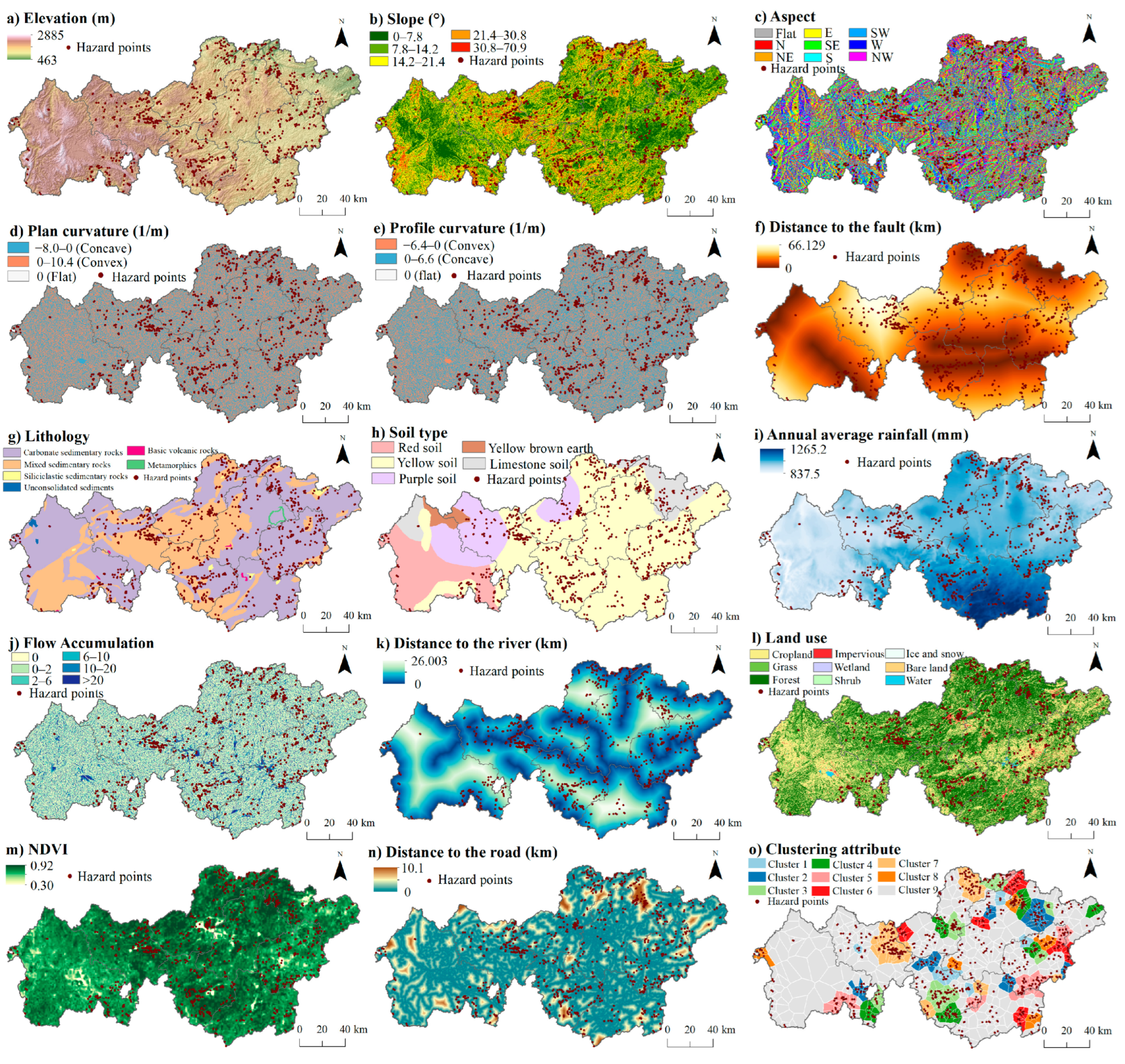
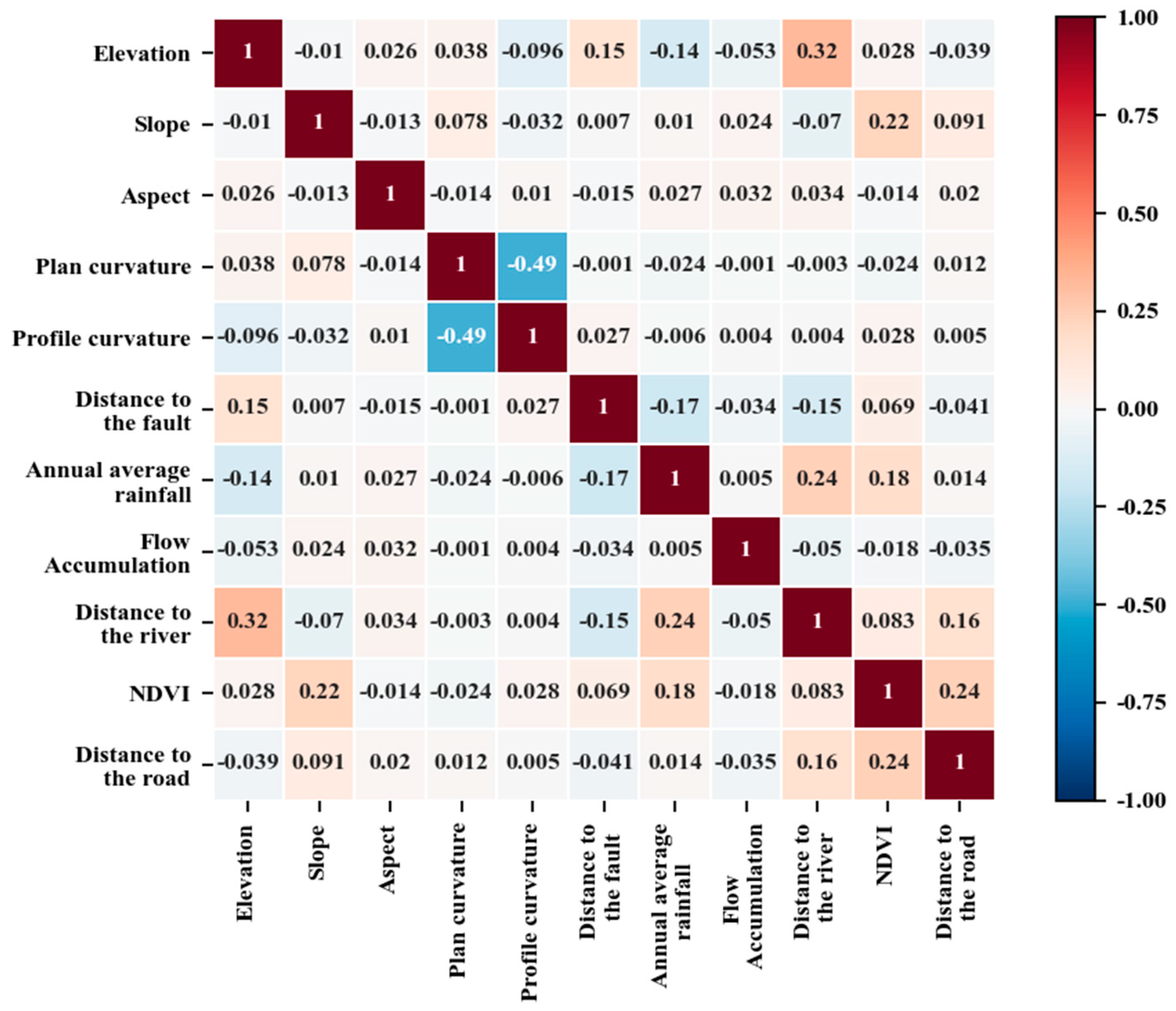
3.1. Constructing the Affecting Factors Data Set

Considering the induced mechanism of landslides, we selected 15 factors from the aspects of topography and geology, soil and hydrology, land cover, human activity, and historical hazards by combining existing studies (

Table 1. Introduction of affecting factors *.

Dimensions	Affecting Factor	Original Resolution	Resampling Technique	Data Source
Topography	Elevation	90 m	-	SRTMDEM (90 m) from Geospatial Data Cloud (http://www.gscloud.cn/ (accessed on 16 April 2022))
	Slope	-	-	Calculated from elevation
	Aspect	-	-
	Plan curvature	-	-
	Profile curvature	-	-
Geology	Distance to the fault	-	-	Fault data from Seismic Active Fault Survey Data Center (http://www.activefault-datacenter.cn/ (accessed on 16 April 2022))
	Lithology	Vector	-	The global lithological map database GLiM (https://doi.org/10.1594/PANGAEA.788537 (accessed on 16 April 2022)) [47]
	Soil type	Vector	-	Resource and Environment Science and Data Center (https://www.resdc.cn/ (accessed on 16 April 2022))
Hydrology	Annual average rainfall	1 km	Bilinear interpolation	Resource and Environment Science and Data Center
	Flow accumulation	-	-	Calculated from elevation
	Distance to the river	-	-	River data from OpenStreetMap (https://www.openstreetmap.org/ (accessed on 16 April 2022))
Land cover	Land use	10 m	Nearest neighbor	Finer Resolution Observation and Monitoring-Global Land Cover (http://data.ess.tsinghua.edu.cn/ (accessed on 16 April 2022)) [48]
	NDVI	1 km	Bilinear interpolation	Resource and Environment Science and Data Center
Human activity	Distance to the road	-	-	Road data from OpenStreetMap (https://www.openstreetmap.org/ (accessed on 16 April 2022))
Historical hazards	Clustering attribute	-	-	Calculated from historical hazard points

* Note: Lithology, soil type, land use, and clustering attribute are categorical variables, and the others are continuous. Distance to the fault, river, and road are the Euclidean distance to the nearest target.

). The spatial distribution map of affecting factors (Figure 6) was drawn based on the WGS_1984_UTM_Zone_48N coordinate system with a resolution of 90 × 90 m. The number of grid rows and columns were 1763 and 3475, respectively, and the total number of grids was 3,389,074. A more detailed explanation on how these factors in Table 1 influence landslide susceptibility is elaborated on in the Supplementary Materials.

If there was a strong collinearity among the affecting factors, the noise from the redundant information would interfere with the model. Therefore, collinearity analysis was essential. Common applied methods for collinearity validation include correlation analysis and the variance inflation factor (VIF) [21,49]. The former concerns the collinearity between two variables, while the latter focuses on the multicollinearity between one variable and other variables. Here, we adopted the Pearson correlation coefficient for correlation analysis, in which values greater than 0.7 are considered to have a strong pairwise collinearity, and tolerance (TOL) and the VIF (the reciprocal of TOL) for multicollinearity analysis, where a TOL less than 0.1 and VIF greater than 10 indicate a serious multicollinearity problem [50,51].

The Pearson correlation requires two variables to be continuous, so the four factors of lithology, soil type, land use, and clustering attribute were excluded from this analysis. All values in the correlation coefficient matrix (Figure 7) were less than 0.7, while the values for TOL ranged from 0.356 to 0.994, and the values for the VIF ranged from 1.006 to 2.807 (

Table 2. Multicollinearity results of affecting factors.

Affecting Factor	TOL	VIF	Affecting Factor	TOL	VIF
Elevation	0.425	2.353	Annual average rainfall	0.453	2.207
Slope	0.771	1.297	Flow accumulation	0.984	1.016
Aspect	0.994	1.006	Distance to the river	0.448	2.234
Plan curvature	0.362	2.762	NDVI	0.545	1.835
Profile curvature	0.356	2.807	Distance to the road	0.781	1.280
Distance to the fault	0.791	1.264	-	-	-

), illustrating there was no collinearity among the affecting factors. It is notable the Pearson correlation coefficient is only a measure of linear correlation and sensitive to outliers. Considering there are some coefficient values in Figure 7 close to zero, this result may ignore other types of relationships or correlations. Thus, we supplemented Spearman’s correlation coefficient and the distance correlation between 15 affecting factors as well as the output variable in the Supplementary Materials. The corresponding results also indicated no significant linear or nonlinear association among any variables. We can presume that the factor selection was feasible.

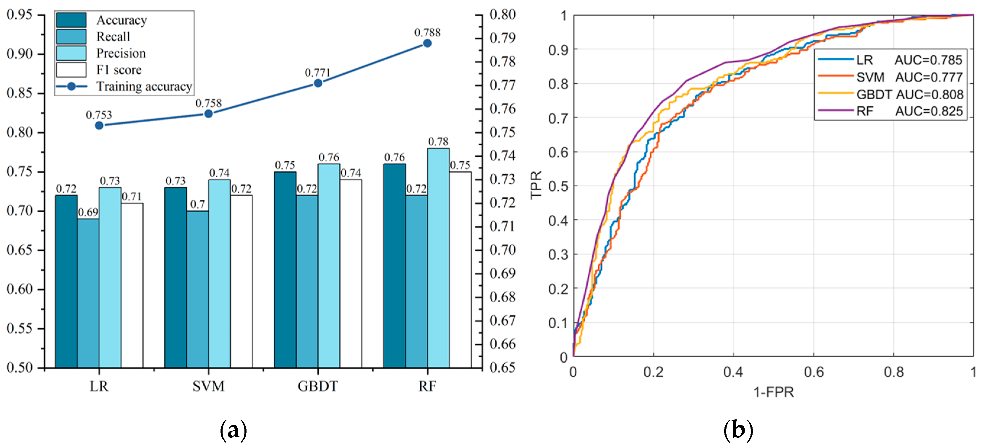
3.2. Evaluation of Model Prediction Accuracy

Based on the input of the affecting factors dataset and training set, models were built and run in MATLAB (Version: 2020b; Copyright: The Math Works, Inc. [52]). Then, the performance of each model in the test set was evaluated in terms of the statistical indexes, ROC curve (Figure 8), and confusion matrix (

Table 3. The confusion matrix for each model in the test set.

	Number	$\mathit{T}\mathit{P}$	$\mathit{F}\mathit{N}$	$\mathit{T}\mathit{N}$	$\mathit{F}\mathit{P}$
Model
LR		208	93	225	76
SVM		210	91	227	74
GBDT		218	83	232	69
RF		217	84	240	61

).

The highest index values of RF in Figure 8a, including the training accuracy (78.8%), test $accuracy$, and $precision$ (76% and 78%, respectively), suggest that the RF model outperformed the others both in the training and test sets. This means that the proportion of positive and negative samples correctly predicted in the RF test results was 76%, with 78% of the predicted hazard points being actual points. However, the $recall$ of the RF model, one indicator describing the proportion of correctly predicted hazard points of all actual points, was relatively low at 72%. Higher $F1 scores$ for the RF and GBDT models revealed a notable conclusion that the integrated algorithms with decision tree-based classifiers performed significantly better than traditional machine learning algorithms such as LR and the SVM. That aside, the training and test accuracy of each model were approximate, representing no overfitting or underfitting. The overall prediction accuracy was quite acceptable, as the AUC values of all four models reached above 0.77 (Figure 8b). The RF model achieved the highest AUC value of 0.825. Meanwhile, combined with the confusion matrix, GBDT as an integrated algorithm slightly outperformed RF in terms of hazard point recognition. Nevertheless, it clearly underperformed on non-hazard points compared with RF. Ultimately, the RF model was the optimal model for the prediction accuracy in this study.

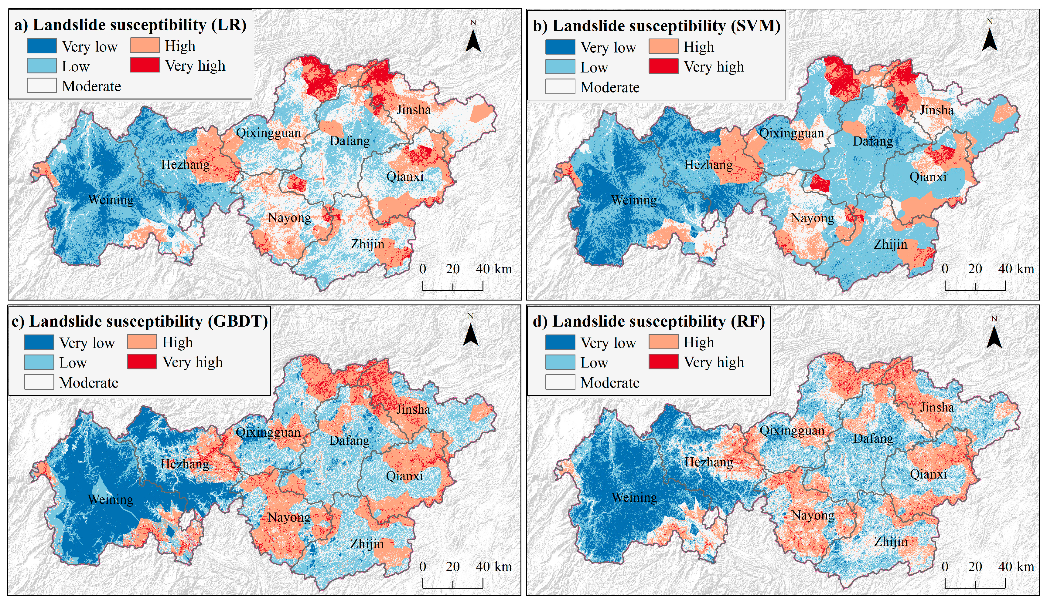
3.3. Mapping the Landslide Susceptibility

According to the models constructed above, we predicted the probability of hazard occurrence ($p$) for each raster cell to draw landslide susceptibility maps for Bijie (Figure 9) and divide the susceptibility into five levels: very low (0 ≤ p ≤ 0.1), low (0.1 < p ≤ 0.3), moderate (0.3 < p ≤ 0.6), high (0.6 < p ≤ 0.9), and very high (0.9 < p ≤ 1). Then, the map reliability was assessed by the quality of the presented information and the indicators in Figure 10. Consistent with the accuracy prediction findings above, the susceptibility map produced by a RF algorithm had a better simulation effect, as reflected by the following:

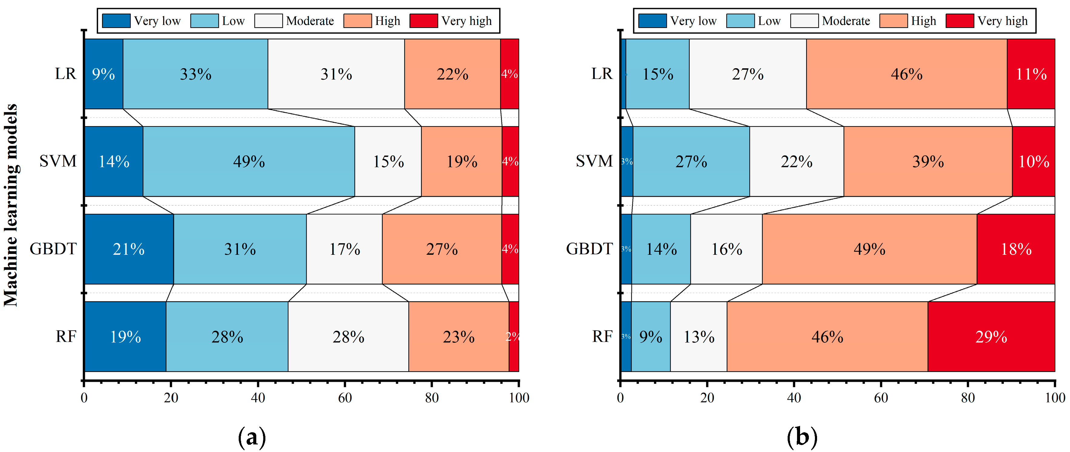
• At the global scale, the spatial distribution and area shares of different levels of susceptibility were more reasonable than those of other methods. For example, the very high susceptibility areas were moderately distributed among the high-value areas of each county (Figure 9d), whereas for LR and the SVM, the very high susceptibility areas were concentrated in blocks in the northernmost areas of Bijie, southwest of Dafang, and northeast of central Qianxi, featuring a local exaggeration which was biased from reality, being especially overestimated in the southwest of Dafang, where there were only six hazard points (Figure 9a,b). For GBDT, the percentage of moderately prone areas was underrepresented, accounting for 17% (Figure 10a).
• At the local scale, the RF map was richer in spatial details and retained a gradual change in susceptibility from high to low in the high-value areas, which is realistic. In contrast, the other three maps were more distinctly patchy, with coarser portrayals of the highly and less prone areas.
• In terms of the interpretation effect of historical hazards, the more-prone areas (including high and very high areas, the same as those shown below) representing 25% of the RF map area contained 75% of the historical hazard points, and the less-prone areas (including low and very low areas, the same as those shown below) representing 47% of the RF area contained only 12% of the hazard points (Figure 10). This strongly proves the capability of the RF map to effectively reflect the true state of susceptibility. However, other maps did not perform as well, such as the GBDT map with a larger proportion of more-prone areas (31%) which explained only 67% of the historical hazards, while the SVM map with less-prone areas (63%) over-explained 30% of the hazards.

Considering the prediction accuracy and mapping effect above, it can be concluded that the LR and SVM models performed similarly in this study and were inferior to the integrated models of GBDT and RF due to the problem of large prediction bias in the more-prone areas. GBDT, although functioning analogously with RF, tended to predict toward the extreme end (i.e., dividing higher or lower values for raster cells), which would result in a skewed distribution. Therefore, we eventually recognized the RF map as the ideal landslide susceptibility situation in Bijie, which was closest to the historical distribution. Derived from it, the overall susceptibility of the city could be attributed to the characteristics of high in the east, low in the west, and frequent regional occurrences. The more-prone areas on alert covered a wide range of Bijie, focusing on the central (Nayong, to the east of Hezhang), northeastern (the intersection of Jinsha, Dafang, and Qixingguan), eastern (north of central Qianxi and the intersection of Qianxi and Zhijin), and southwestern (south of Weining) areas of Bijie.

As disaster risk management is generally implemented at the county administrative level, it is necessary to further analyze the susceptibility at the county level to support decision making. Based on the numerical distribution of hazard occurrence probability in all raster cells of each county (Figure 11a), the counties in Bijie can be ranked as three echelons according to the susceptibility level from high to low: the first echelon (Nayong, Qianxi, Jinsha, and Qixingguan), second echelon (Zhijin, Dafang, and Hezhang), and third echelon (Weining). Reflected by the violin plot width (Figure 11a) and proportion of the sector area (Figure 11b), the counties in first echelon were distinguished by a large proportion and area of higher susceptibility, which should be given priority for monitoring and prevention. Among them, Nayong was the most severe one because it only had a sole peak at the high value of probability, compared with the other counties with bimodal distribution in the high and low values (Figure 11a). The overall susceptibility of counties in the second echelon moderately decreased, as evidenced by the mean and median being at the medium level of occurrence probability and the sole peak at the lower value. However, the aggregation of the more-prone areas situated in the local areas deserve attention. For example, the very high susceptibility area in Hezhang is still vast (Figure 11b), so these similar local blocks of high value in the second echelon should be the focus of further investigation. With the high elevation and wide area in the central zone, landslides rarely happened in central Weining in the third echelon. Instead, it developed a distinctive polarization of susceptibility, and thus the main work on future disaster prevention and mitigation planning is advised to be devoted to some higher susceptibility areas to its southeast and northwest.

In China, the landslide susceptibility map was a critical basis for prevention activities. With efforts in the 12th Five-Year Plan (2010–2015), the comprehensive treatment of geohazards achieved such remarkable results as a reduction of 316,000 casualties, a decrease of 67% over the 11th Five-Year Plan. A susceptibility assessment map with higher accuracy in high susceptibility areas at the city or county level may further improve future prevention effectiveness.

4. Discussion

4.1. Impact of the Spatial Clustering Attribute on the Models

Through the above analyses, it is clear that there exists a significant spatial clustering of landslides in Bijie. The importance for each factor of the RF model (Figure 12a) indicates that the clustering attribute contributed the most to the model, followed by topographic and geological, hydrological, and human activity factors such as elevation, distance to the river, fault, and road, and the annual average rainfall. Meanwhile, this high contribution of the clustering attribute also accounted for the formation of the spatial distribution pattern of high-value areas in the susceptibility map. In order to quantify the impact of the spatial clustering characteristic on the model performance, the clustering attribute was eliminated from the affecting factors data set and remodeled to obtain ROC curves for each model (Figure 12b). Taking the optimal RF model as an example, we measured the actual utility of considering spatial agglomeration by comparing the confusion matrix, accuracy indexes, and simulated map validity (

Table 4. Comparison of confusion matrices and accuracy indexes of the test set before and after exclusion (RF).

Number	Before	After	Index	Before	After
$TP$	217	216	$Accuracy$	0.76	0.71
$FN$	84	85	$Recall$	0.72	0.72
$TN$	240	214	$Precision$	0.78	0.71
$FP$	61	87	$F1 score$	0.75	0.72

and Figure 12c,d) before and after exclusion.

After the exclusion, the training accuracy of the RF model decreased from 78.8% to 72.0%, and the $accuracy$, $precision$, and $F1 score$ of the test set were also greatly reduced (Table 4). Additionally, the AUC values of the four models in Figure 12b dropped significantly (RF from 0.825 to 0.793). The unfavorable changes in these metrics demonstrate that considering the spatial agglomeration feature can effectively improve the model’s prediction accuracy.

On the other hand, the number of $TP$s, $FN$s, and the $recall$ value in Table 4 remained basically unchanged before and after exclusion, while the number of $TN$s and $FP$s changed significantly. It enlightens us that the gaining effect of the agglomeration on the model was mainly in the more accurate discrimination of non-hazard points, as more non-hazard points were correctly identified. Consequently, a model simulation result that does not take into account the agglomeration feature tends to overestimate the susceptibility of less-prone areas and underestimate that of more-prone areas indirectly. Considering that disaster mitigation resources are always limited, accurately delineating the high-susceptibility area of greater concern is critical in planning. This inference is also supported by the comparison of spatial distribution patterns of susceptibility in Figure 9d and Figure 12c, as the less-prone areas (representing non-hazard points correctly identified) after exclusion had very little coverage in central Bijie, while the more- or less-prone areas before exclusion were more reasonably distributed.

The area percentages of the more- and less-prone areas after exclusion decreased significantly from 25% and 47% to 18% and 34%, respectively (Figure 12d), and the more-prone area distribution ended in unacceptable spatial decentralization and homogenization (Figure 12c). In the meantime, this inferior map had the problem of biased estimation and inaccurate judgment of critical hazard areas, as reflected in the failure to identify partially hazard-prone areas (such as south of Nayong and southeast of Zhijin) and the overestimation of local less-prone areas (such as south of Dafang). Furthermore, the exclusion of the clustering attribute remarkably reduced the interpretation of more-prone areas to the historical hazard points by 15% (from 75% to 60%). Despite a 4% reduction (from 12% to 8%) in the interpretation of less-prone areas to hazards, the great reduction of 13% in its area it should be taken into account. Therefore, the final simulation performance of the model after eliminating the clustering attribute was obviously cut down.

In summary, the spatial agglomeration feature had a significant positive impact on improving the models.

4.2. Impact of the Spatial Dispersion Characteristic on the Models

Given that the dispersion characteristic may have a negative effect on model’s prediction, this paper filtered the original hazard inventory and generated the test set based on the fishnet grid proposed. In order to verify the effectiveness of the data preprocessing method, we took no action on the raw data and still divided the training and test sets according to the ratio of 70% and 30% before generating the equal number of non-hazard points without the constraint of a fishnet grid. As shown in Figure 13a, the number of training and test set points were both 1267, and meanwhile, blue non-hazard points fell randomly within the red fishnet grid area, while outside the grid, red hazard points which were filtered before existed.

As expected, the prediction accuracy of each model decreased significantly according to the ROC curve, especially evidenced by the AUC value of the RF model dropping from 0.825 to 0.716 and its training accuracy reaching only 66.3%. Simultaneously, the advantage of the integrated algorithm was no longer obvious compared with the LR and SVM models (Figure 13b). The four accuracy indexes all reduced dramatically by around 10% (

Table 5. Comparison of confusion matrices and accuracy indexes of test set with or without preprocessing (RF).

Number	With	Without	Index	With	Without
$TP$	217	250	$Accuracy$	0.76	0.66
$FN$	84	130	$Recall$	0.72	0.66
$TN$	240	251	$Precision$	0.78	0.66
$FP$	61	129	$F1 score$	0.75	0.66

), which further revealed the prominent availability of a fishnet grid preprocessing scheme in improving the model.

Similar to the drawbacks of the map in Figure 12c, there were also several problems in the map depicted without using a fishnet grid in Figure 13c, and they are as follows:

• There was an unreasonable allocation of area for the different susceptibility levels, which was reflected both in the area percentage and the spatial distribution. Specifically, the area percentages of the more- and less-prone areas distinctly decreased by 6% and 13%, respectively, while that of the moderate susceptibility areas increased steeply to 47% (Figure 13d). Combined with reality, it seems to be too aggressive to state that nearly half the area of Bijie is moderately susceptible. Secondly, the overall spatial distribution also suffered from the problem of overestimation in the less-prone areas and underestimation in the more-prone areas, as shown in Figure 12c, and could not portray the gradual change in susceptibility between neighborhoods, as shown in Figure 9d.
• There was weakening of the interpretation effect on historical hazards. This manifested in the sharp 11% reduction in the interpretation of the very high susceptibility areas. Despite an 8% increase in the interpretation of the more-prone areas, there was an unexpected decrease in the relative proportion of very high susceptibility areas in the more-prone areas in the interpretation rate from 39% to 22%, as this went against the nature of more hazards occurring at the very high susceptibility level. However, the interpretation effect of the less-prone areas improved with a 10% reduction. The reason behind this was that without preprocessing for filtering, those isolated hazard points representing less-prone levels were fully learned by the model, thus contributing a better interpretation for the less-prone areas but at the expense of the overall accuracy. The loss of the interpretation rate of low susceptibility areas actually reflected the loss of data due to the filtration of isolated points. Compared with the improvement to the whole evaluation’s effectiveness, especially in the high susceptibility area, the data loss was acceptable.

Overall, the preprocessing scheme of the fishnet grid we constructed could remarkably raise the model prediction accuracy and optimize the spatial evaluation results. Although it may force the model to lose some of its interpretation rate in low susceptibility areas, the overall spatial pattern of susceptibility would not be influenced and retain values close to the actual ones. After all, high susceptibility areas always deserve more attentions. Consequently, when applied to other regions, the filtering scale of a fishnet grid can be adjusted according to the historical data to maximize the prediction accuracy with minimal compromising of the interpretation rate. The experiment also proved our inference that the dispersion would cause a biased prediction.

5. Conclusions

Facing the challenge of increased geohazard risk under urbanization and climate change, in-depth understanding of high landslide susceptibility areas is critical to life and asset safety. Committed to this, and taking the city of Bijie in southwestern China with serious landslides as a case, we assessed its susceptibility and discussed the possibility of using information from the landslide data from the perspective of the often-overlooked spatial distribution characteristics of the hazards. The main contribution of our work is that we developed a new reinforcement strategy based on the spatial agglomeration and dispersion features of landslides, which can rectify the possible systematic bias of overestimating low susceptibility areas and underestimating high susceptibility areas in previous assessments, which improves the assessment accuracy and effectiveness, especially in high susceptibility regions. Specifically, the strategy includes clustering attribute extraction derived from the OPTICS algorithm (for spatial agglomeration) and a data preprocessing method based on the fishnet grid (for spatial dispersion). Further experiments demonstrated that the neglect of these two spatial features reduced the reliability of the assessment outcome. Our detailed findings are summarized as follows:

• Indicator selection: Adding a spatial clustering attribute as one affecting factor can effectively enhance the model’s ability to recognize non-hazard points and in turn increase the model’s accuracy by nearly 5%. Most importantly, it corrects for the formerly unnoticed systematic assessment bias. The improvements in accurate identification in higher susceptibility areas and interpretation to historical hazards will help optimize the deployment of disaster prevention structures.
• Data processing: When using the fishnet grid as a mask to process the original data, the entire spatial pattern of susceptibility will not change, the training and testing accuracies will be improved by about 10%, and the spatial division of each susceptibility level will be more in line with the historical data, which may better serve disaster monitoring and control in the real world.
• Model construction: The integrated algorithms represented by the RF and GBDT algorithms outperformed the traditional ones such as LR and the SVM. Among them, the RF model was the best, with its $accuracy$ of up to 76% and $precision$ of up to 78%. Moreover, the superiority of the RF map lies in the more accurate positioning of higher susceptibility areas globally and the richer spatial portrayal of susceptibility locally, which reflects the necessary spatial group-occurring, inter-regional heterogeneity, and gradual variability characteristics of susceptibility.
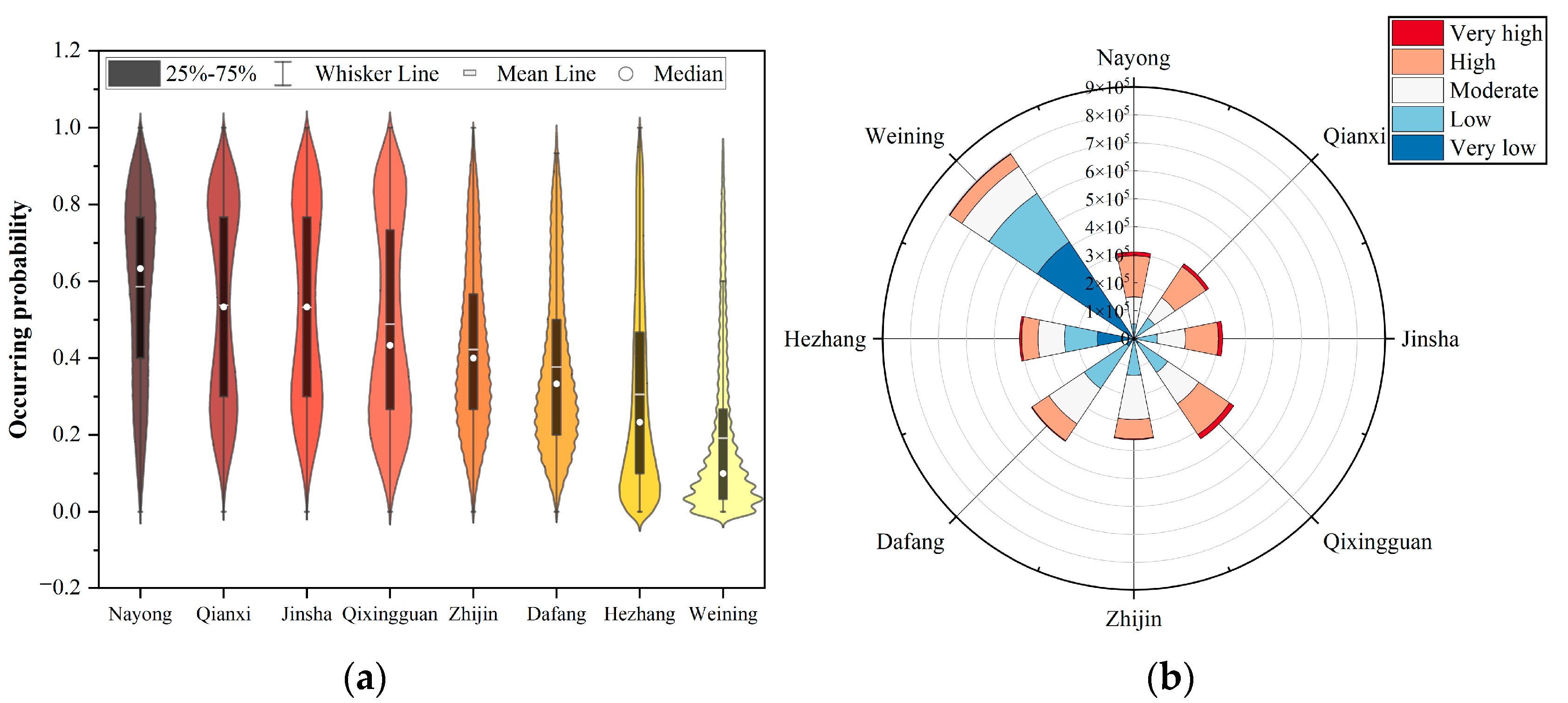
• Management suggestion: The landslide susceptibility in Bijie presented a high susceptibility in the east, low susceptibility in the west, and a regional clustering pattern, with its central, northeastern, eastern edge, and southwestern areas having a high susceptibility level. The counties in Bijie can be divided into three echelons in descending order of susceptibility. For the first echelon, with a wide range and large proportion of more-prone areas, an adequate professional inspection of the geological environment should be implemented in place as a priority before regular slope monitoring and stabilization measures. Despite a moderate reduction in the susceptibility degree for the second and third echelons, the regional concentrations of high-susceptibility areas still deserve particular attention and warrant relevant authorities taking actions to develop adaptive development strategies for balancing human activities and the natural environment.

For geological hazard-prone countries and regions with vast land and complicated topographies, the resources for risk reduction are always limited. The accurate recognition of high landslide susceptibility achieved by our strategy is instructive to the field survey for hidden hazard areas and the investment of risk prevention measures for high susceptibility areas with dense populations and assets. Certainly, there are still limitations to this study in some aspects, such as the absence of consideration of time-varying factors, the uncertainty of the global optimal solution of the search distance in the clustering algorithm, and the lack of case validation in other regions. We will expand this study from these aspects and refine our model through developing hybrid algorithms for higher accuracy and quality simultaneously.

References

1. Aleotti, P.; Chowdhury, R. Landslide hazard assessment: Summary review and new perspectives. Bull. Eng. Geol. Environ. 1999, 58, 21–44. [Google Scholar] [CrossRef]
2. Sepúlveda, S.A.; Rebolledo, S.; Vargas, G. Recent catastrophic debris flows in Chile: Geological hazard, climatic relationships and human response. Quatern. Int. 2006, 158, 83–95. [Google Scholar] [CrossRef]
3. Cui, P. Progress and prospects in research on mountain hazards in China. Prog. Geogr. 2014, 33, 145–152. [Google Scholar]
4. Donat, M.G.; Lowry, A.L.; Alexander, L.V.; O Gorman, P.A.; Maher, N. More extreme precipitation in the world’s dry and wet regions. Nat. Clim Chang. 2016, 6, 508–513. [Google Scholar] [CrossRef]
5. Shi, P.; Yang, W. Compound effects of earthquakes and extreme weathers on geo-hazards in mountains. Clim. Chang. Res. 2020, 16, 405. [Google Scholar]
6. Yesilnacar, E.; Topal, T. Landslide susceptibility mapping: A comparison of logistic regression and neural networks methods in a medium scale study, Hendek region (Turkey). Eng. Geol. 2005, 79, 251–266. [Google Scholar] [CrossRef]
7. Chen, W.; Peng, J.; Hong, H.; Shahabi, H.; Pradhan, B.; Liu, J.; Zhu, A.; Pei, X.; Duan, Z. Landslide susceptibility modelling using GIS-based machine learning techniques for Chongren County, Jiangxi Province, China. Sci. Total Environ. 2018, 626, 1121–1135. [Google Scholar] [CrossRef]
8. Yilmaz, I.; Keskin, I. GIS based statistical and physical approaches to landslide susceptibility mapping (Sebinkarahisar, Turkey). Bull. Eng. Geol. Environ. 2009, 68, 459–471. [Google Scholar] [CrossRef]
9. Stamatopoulos, C.A.; Di, B. Analytical and approximate expressions predicting post-failure landslide displacement using the multi-block model and energy methods. Landslides 2015, 12, 1207–1213. [Google Scholar] [CrossRef]
10. Nie, Y.; Li, X.; Zhou, W.; Xu, R. Dynamic hazard assessment of group-occurring debris flows based on a coupled model. Nat. Hazards 2021, 106, 2635–2661. [Google Scholar] [CrossRef]
11. Goetz, J.N.; Guthrie, R.H.; Brenning, A. Integrating physical and empirical landslide susceptibility models using generalized additive models. Geomorphology 2011, 129, 376–386. [Google Scholar] [CrossRef]
12. Liu, C.; Li, W.; Wu, H.; Lu, P.; Sang, K.; Sun, W.; Chen, W.; Hong, Y.; Li, R. Susceptibility evaluation and mapping of China’s landslides based on multi-source data. Nat. Hazards 2013, 69, 1477–1495. [Google Scholar] [CrossRef]
13. Tan, Y.; Guo, D.; Xu, B. A geospatial information quantity model for regional landslide risk assessment. Nat. Hazards 2015, 79, 1385–1398. [Google Scholar] [CrossRef]
14. Panchal, S.; Shrivastava, A.K. A comparative study of frequency ratio, Shannon’s entropy and analytic hierarchy process (AHP) models for landslide susceptibility assessment. ISPRS Int. J. Geo-Inf. 2021, 10, 603. [Google Scholar] [CrossRef]
15. Ding, Q.; Chen, W.; Hong, H. Application of frequency ratio, weights of evidence and evidential belief function models in landslide susceptibility mapping. Geocarto Int. 2017, 32, 619–639. [Google Scholar] [CrossRef]
16. Pourghasemi, H.R.; Pradhan, B.; Gokceoglu, C.; Mohammadi, M.; Moradi, H.R. Application of weights-of-evidence and certainty factor models and their comparison in landslide susceptibility mapping at Haraz watershed, Iran. Arab. J. Geosci. 2013, 6, 2351–2365. [Google Scholar] [CrossRef]
17. He, S.; Pan, P.; Dai, L.; Wang, H.; Liu, J. Application of kernel-based Fisher discriminant analysis to map landslide susceptibility in the Qinggan River delta, Three Gorges, China. Geomorphology 2012, 171, 30–41. [Google Scholar] [CrossRef]
18. Cao, J.; Zhang, Z.; Du, J.; Zhang, L.; Song, Y.; Sun, G. Multi-geohazards susceptibility mapping based on machine learning—a case study in Jiuzhaigou, China. Nat. Hazards 2020, 102, 851–871. [Google Scholar] [CrossRef]
19. Ayalew, L.; Yamagishi, H. The application of GIS-based logistic regression for landslide susceptibility mapping in the Kakuda-Yahiko Mountains, Central Japan. Geomorphology 2005, 65, 15–31. [Google Scholar] [CrossRef]
20. Gao, R.; Wang, C.; Liang, Z.; Han, S.; Li, B. A Research on Susceptibility Mapping of Multiple Geological Hazards in Yanzi River Basin, China. ISPRS Int. J. Geo-Inf. 2021, 10, 218. [Google Scholar] [CrossRef]
21. Cao, J.; Zhang, Z.; Wang, C.; Liu, J.; Zhang, L. Susceptibility assessment of landslides triggered by earthquakes in the Western Sichuan Plateau. Catena 2019, 175, 63–76. [Google Scholar] [CrossRef]
22. Tian, Y.; Xu, C.; Hong, H.; Zhou, Q.; Wang, D. Mapping earthquake-triggered landslide susceptibility by use of artificial neural network (ANN) models: An example of the 2013 Minxian (China) Mw 5.9 event. Geomat. Nat. Hazards Risk 2019, 10, 1–25. [Google Scholar] [CrossRef] [Green Version]
23. Chen, W.; Xie, X.; Peng, J.; Shahabi, H.; Hong, H.; Bui, D.T.; Duan, Z.; Li, S.; Zhu, A. GIS-based landslide susceptibility evaluation using a novel hybrid integration approach of bivariate statistical based random forest method. Catena 2018, 164, 135–149. [Google Scholar] [CrossRef]
24. Pourghasemi, H.R.; Rahmati, O. Prediction of the landslide susceptibility: Which algorithm, which precision? Catena 2018, 162, 177–192. [Google Scholar] [CrossRef]
25. Chen, W.; Xie, X.; Wang, J.; Pradhan, B.; Hong, H.; Bui, D.T.; Duan, Z.; Ma, J. A comparative study of logistic model tree, random forest, and classification and regression tree models for spatial prediction of landslide susceptibility. Catena 2017, 151, 147–160. [Google Scholar] [CrossRef] [Green Version]
26. Marjanović, M.; Kovačević, M.; Bajat, B.; Voženílek, V. Landslide susceptibility assessment using SVM machine learning algorithm. Eng. Geol. 2011, 123, 225–234. [Google Scholar] [CrossRef]
27. Bui, D.T.; Tuan, T.A.; Klempe, H.; Pradhan, B.; Revhaug, I. Spatial prediction models for shallow landslide hazards: A comparative assessment of the efficacy of support vector machines, artificial neural networks, kernel logistic regression, and logistic model tree. Landslides 2016, 13, 361–378. [Google Scholar]
28. Zhang, X.; Li, P.; Li, Z.B.; Yu, G. Characteristics and formation mechanism of the July 25, 2013, Tianshui group-occurring geohazards. Environ. Earth Sci. 2017, 76, 219. [Google Scholar] [CrossRef]
29. Shafizadeh-Moghadam, H.; Minaei, M.; Shahabi, H.; Hagenauer, J. Big data in geohazard; pattern mining and large scale analysis of landslides in Iran. Earth Sci. Inform. 2019, 12, 1–17. [Google Scholar] [CrossRef]
30. Qiu, H.J. Study on the Regional Landslide Characteristic Analysis and Hazard Assessment: A Case Study of Ningqiang County. Ph.D. Thesis, Northwest University, Xi’an, China, 2012. [Google Scholar]
31. Wang, Y.; Feng, L.; Li, S.; Ren, F.; Du, Q. A hybrid model considering spatial heterogeneity for landslide susceptibility mapping in Zhejiang Province, China. Catena 2020, 188, 104425. [Google Scholar] [CrossRef]
32. Yang, Y.; Yang, J.; Xu, C.; Xu, C.; Song, C. Local-scale landslide susceptibility mapping using the B-GeoSVC model. Landslides 2019, 16, 1301–1312. [Google Scholar] [CrossRef]
33. Jacobs, L.; Kervyn, M.; Reichenbach, P.; Rossi, M.; Marchesini, I.; Alvioli, M.; Dewitte, O. Regional susceptibility assessments with heterogeneous landslide information: Slope unit-vs. pixel-based approach. Geomorphology 2020, 356, 107084. [Google Scholar] [CrossRef]
34. Qiu, H.; Cao, M.; Liu, W.; Hao, J.; Wang, Y. Research on the spatial point pattern of geo-hazard—A case of Ningqiang county. J. Arid. Land Resour. Environ. 2014, 28, 107–111. [Google Scholar]
35. Kalantar, B.; Pradhan, B.; Naghibi, S.A.; Motevalli, A.; Mansor, S. Assessment of the effects of training data selection on the landslide susceptibility mapping: A comparison between support vector machine (SVM), logistic regression (LR) and artificial neural networks (ANN). Geomat. Nat. Hazards Risk 2018, 9, 49–69. [Google Scholar] [CrossRef]
36. Lin, J.; Zhang, A.; Deng, C.; Chen, W.; Liang, C. Sensitivity Assessment of Geological Hazards in Urban Agglomeration of Fujian Delta Region. J. Geo-Inf. Sci. 2018, 20, 1286–1297. [Google Scholar]
37. Chen, W.; Li, R.; Yin, Z.; Tang, Z. A study of evaluation of resources and environment carrying capacity of Qixingguan District in Bijie City, Wumeng Mountain, Guizhou Province. Geol. Bull. China 2020, 39, 114–123. [Google Scholar]
38. ESRI. ArcGIS Desktop; Version 10.6; Environmental Systems Research Institute: Redlands, CA, USA, 2018; Available online: https://www.arcgis.com/ (accessed on 17 March 2022).
39. Zhang, N.; Xu, Y.; Yan, H. A study of the instability mechanism and investigation methods of shallow bedrock landslides in Karst mountain areas: Taking the Jinxing landslide in Dafang County as an example. Hydrogeol. Eng. Geol. 2017, 44, 142–146. [Google Scholar]
40. Zheng, G.; Xu, Q.; Ju, Y. The pusacun rockavalanche on August 28, 2017 in Zhanggjiawan Nayongxian, Guizhou: Characteristics and failure mechanism. J. Eng. Geol. 2018, 26, 223–240. [Google Scholar]
41. Xu, S.; Liu, J.; Wang, X. Landslide susceptibility assessment method incorporating index of entropy based on support vector machine: A case study of Shaanxi Province. Geomat. Inf. Sci. Wuhan Univ. 2020, 45, 1214–1222. [Google Scholar]
42. Budimir, M.E.A.; Atkinson, P.M.; Lewis, H.G. A systematic review of landslide probability mapping using logistic regression. Landslides 2015, 12, 419–436. [Google Scholar] [CrossRef] [Green Version]
43. Trigila, A.; Iadanza, C.; Esposito, C.; Scarascia-Mugnozza, G. Comparison of Logistic Regression and Random Forests techniques for shallow landslide susceptibility assessment in Giampilieri (NE Sicily, Italy). Geomorphology 2015, 249, 119–136. [Google Scholar] [CrossRef]
44. Ankerst, M.; Breunig, M.M.; Kriegel, H.; Sander, J. OPTICS: Ordering points to identify the clustering structure. ACM Sigmod Rec. 1999, 28, 49–60. [Google Scholar] [CrossRef]
45. Jiang, W.; Rao, P.; Cao, R.; Tang, Z.; Chen, K. Comparative evaluation of geological disaster susceptibility using multi-regression methods and spatial accuracy validation. J. Geogr. Sci. 2017, 27, 439–462. [Google Scholar] [CrossRef] [Green Version]
46. Lucchese, L.V.; de Oliveira, G.G.; Pedrollo, O.C. Investigation of the influence of nonoccurrence sampling on landslide susceptibility assessment using Artificial Neural Networks. Catena 2021, 198, 105067. [Google Scholar] [CrossRef]
47. Hartmann, J.; Moosdorf, N. The new global lithological map database GLiM: A representation of rock properties at the Earth surface. Geochem. Geophys. Geosyst. 2012, 13, 12. [Google Scholar] [CrossRef]
48. Gong, P.; Liu, H.; Zhang, M.; Li, C.; Wang, J.; Huang, H.; Clinton, N.; Ji, L.; Li, W.; Bai, Y.; et al. Stable classification with limited sample: Transferring a 30-m resolution sample set collected in 2015 to mapping 10-m resolution global land cover in 2017. Sci. Bull. 2019, 64, 370–373. [Google Scholar] [CrossRef] [Green Version]
49. He, Q.; Wang, M.; Liu, K. Rapidly assessing earthquake-induced landslide susceptibility on a global scale using random forest. Geomorphology 2021, 391, 107889. [Google Scholar] [CrossRef]
50. Dormann, C.F.; Elith, J.; Bacher, S.; Buchmann, C.; Carl, G.; Carré, G.; Marquéz, J.R.G.; Gruber, B.; Lafourcade, B.; Leitão, P.J.; et al. Collinearity: A review of methods to deal with it and a simulation study evaluating their performance. Ecography 2013, 36, 27–46. [Google Scholar] [CrossRef]
51. Pourghasemi, H.R.; Moradi, H.R.; Fatemi Aghda, S.M. Landslide susceptibility mapping by binary logistic regression, analytical hierarchy process, and statistical index models and assessment of their performances. Nat. Hazards 2013, 69, 749–779. [Google Scholar] [CrossRef]
52. The Math Works, Inc. MATLAB Version 2020b; The Math Works, Inc.: Natick, MA, USA, 2020; Available online: https://www.mathworks.com/ (accessed on 17 March 2022).
Figure 1. Overview of the study area. The landslide events in this data set are divided into 3 categories: collapse, landslide, and debris flow. (Illustrations of the landslide in Dafang and the collapse in Nayong are cited by Zhang et al. [39] and Zheng et al. [40], respectively).
Ijgi 11 00269 g001
Figure 2. Framework of proposed method.
Ijgi 11 00269 g002
Figure 3. The training accuracy test of different parameter combinations of each model based on OPTICS. (a) Training accuracy under different minimum number of points (search distance fixed at 5 km). (b) Training accuracy under different search distances (minimum number of points fixed at 6).
Ijgi 11 00269 g003
Figure 4. Clustering attribute derived from spatial agglomeration based on OPTICS. The results here correspond to the combination of 6 as the minimum number of points and 5 km as the search distance. (a) Clustering results of hazard points based on OPTICS. (b) Clustering attribute of Thiessen polygons based on point clustering results.
Ijgi 11 00269 g004
Figure 5. Data preprocessing method based on the fishnet grid and the generation of the training and test sets. (a) Data preprocessing method based on the fishnet grid. (b) Generating the training set. (c) Generating the test set.
Ijgi 11 00269 g005
Figure 6. The spatial distribution map of affecting factors in Bijie.
Ijgi 11 00269 g006
Figure 7. Pearson correlation coefficient matrix of affecting factors.
Ijgi 11 00269 g007
Figure 8. Evaluation of the prediction accuracy of each model. (a) Statistical accuracy indexes of each model. (b) ROC curve and AUC value of each model.
Ijgi 11 00269 g008
Figure 9. Landslide susceptibility map based on different machine learning models.
Ijgi 11 00269 g009
Figure 10. Percentages of area and historical hazard points in different susceptibility levels. (a) Percentages of area in different susceptibility levels. (b) Percentages of hazard points located in different susceptibility levels. The percentage of hazard points located in the very low area in the LR map is 1%.
Ijgi 11 00269 g010
Figure 11. Landslide susceptibility statistics at the county level in Bijie. (a) Numerical distributions of hazard occurrence probability in all raster cells of each county. (b) Numbers of raster cells in different susceptibility levels of each county. For (a), the two ends of the whisker line are the maximum and minimum values of the corresponding box plot, and the width of the violin plot reflects the density of data at that location, with a greater width representing a greater density.
Ijgi 11 00269 g011
Figure 12. The susceptibility map of Bijie and model performance after excluding the clustering attribute. (a) The importance of factors in the RF model before exclusion. (b) ROC curves and AOC values of each model after exclusion. (c) The landslide susceptibility map after exclusion. (d) Comparison of models’ simulated effects before and after exclusion (the percentage of area in the very high level after exclusion was 0.35%, and the percentage of points in the very low level after exclusion was 2%).
Ijgi 11 00269 g012
Figure 13. The susceptibility map of Bijie and model performance after removing the data preprocessing of the fishnet gird. (a) Distribution of training and test sets without fishnet grid processing. (b) ROC curves and AUC values without fishnet gird processing. (c) The susceptibility map without fishnet grid processing. (d) Comparison of models’ simulated effects before and after processing (the percentage of area in the very high level without preprocessing was 0.25%, and the percentage of hazard points located in the very low level without preprocessing was 0.39%).
Ijgi 11 00269 g013