An Information Fusion Model between GeoSOT Grid and Global Hexagonal Equal Area Grid

Abstract

In order to cope with the rapid growth of spatiotemporal big data, data organization models based on discrete global grid systems have developed rapidly in recent years. Due to the differences in model construction methods, grid level subdivision and coding rules, it is difficult for discrete global grid systems to integrate, share and exchange data between different models. Aiming at the problem of information fusion between a GeoSOT grid and global hexagonal equal area grid system, this paper proposes the GeoSOT equivalent aggregation model (the GEA model). We establish a spatial correlation index method between GeoSOT grids and global hexagonal equal area grids, and based on the spatial correlation index, we propose an interoperable transformation method for grid attributes information. We select the POI (points of interest) data of Beijing bus and subway stations and carry out the transformation experiment of hexagonal grid to GeoSOT grid information so as to verify the effectiveness of the GEA model. The experimental results show that when the 17th-level GeoSOT grid is selected as the particle grid to fit the hexagonal grid, the accuracy and efficiency can be well balanced. The fitting accuracy is 95.51%, and the time consumption is 30.9 ms. We establish the associated index of the GeoSOT grid and the hexagonal grid and finally realized the exchange of information.

1. Introduction

With the development of sensor equipment and geospatial information technology, fast and easy data acquisition methods have surpassed the ability of data processing, which makes the contradiction between data acquisition and processing more prominent. In addition, these data are not uniformly distributed in the spatiotemporal domain, resulting in a particularly large amount of data in a local area, which has the characteristics of typical spatiotemporal big data [1,2].

In order to cope with the agglomeration effect and uneven regional distribution of spatiotemporal big data, methods for organizing and managing spatiotemporal data have developed rapidly [3]. The spatiotemporal data model has developed from the vector raster data model oriented to points, lines, and surfaces, to the object-oriented, process and event-oriented data management method [4,5,6], and then to the subdivision data model suitable for spatiotemporal big data organization. The proposal of the distributed database provides a new solution for the organization of multi-source spatiotemporal data.

With the increase in the amount of spatiotemporal big data, the discrete global grid theory has been developed and perfected rapidly, and corresponding models have been generated in combination with specific application scenarios in their respective fields [7]. Each discrete global grid system has the characteristics of uniqueness, multi-level and efficient coding and calculation. Therefore, discrete global grid systems play a huge advantage in the organization and management of global spatiotemporal big data, and it has been applied in the distributed storage and coding calculation of data.

The discrete global grid system can be constructed according to different methods [8,9,10], such as the global grid model based on latitude and longitude division and the grid model based on polyhedron. The global grid location framework based on the latitude and longitude grid uses regular longitude and latitude lines to recursively divide the surface into several grid cells. This is the earliest and most widely used type of grid framework, which is mainly used to express the location of geographic areas with general precision. Representative models include the “United States National Grid” (USNG) proposed by the US Federal Geographic Data Commission, “British National Grid Reference” (BNGR) proposed by the British Ordnance Survey, and the GBT12409-2009 “Geographic Grid” proposed by China.

The grid model based on polyhedron projects the edges of the sphere-inscribed regular polyhedron (tetrahedron, hexahedron, octahedron, dodecahedron and icosahedron) onto the sphere to cover the surface of the earth [9]. Then, global recursive subdivision is carried out, and the finally formed spherical hierarchical grid structure has the characteristics of approximately uniformity and global continuity. It not only overcomes the defect of singularity of latitude and longitude poles but also overcomes the defect of grid inhomogeneity. The grid is stable, seamless, and approximately uniform on a global scale, and it is currently one of the more effective tools for constructing a global hierarchical grid model. Among them, spherical triangle, rhombus and hexagon are the most popular spherical subdivision elements.

Different discrete global grid systems have different spatial shapes, distributions and arrangements of grid cells that store data as well as significant differences in grid hierarchical division and coding rules. This makes it difficult to integrate and share data under different subdivision methods, and it is also hard to develop cross-system business collaboration.

The Open Geospatial Consortium (OGC) began to formulate the Discrete Global Grid System Core Standard in 2014, trying to establish an open grid location framework to achieve interoperability between different grids [11]. The standard proposed by OGC considers the grid to be just the information framework, ignoring that the grid is the attribute of the location framework. In addition, the standard fails to establish a theoretically complete subdivision coding model, and it lacks an operable grid coding operation definition and geometric feature evaluation method, which makes it difficult to guide the interoperability and practical application of grid systems.

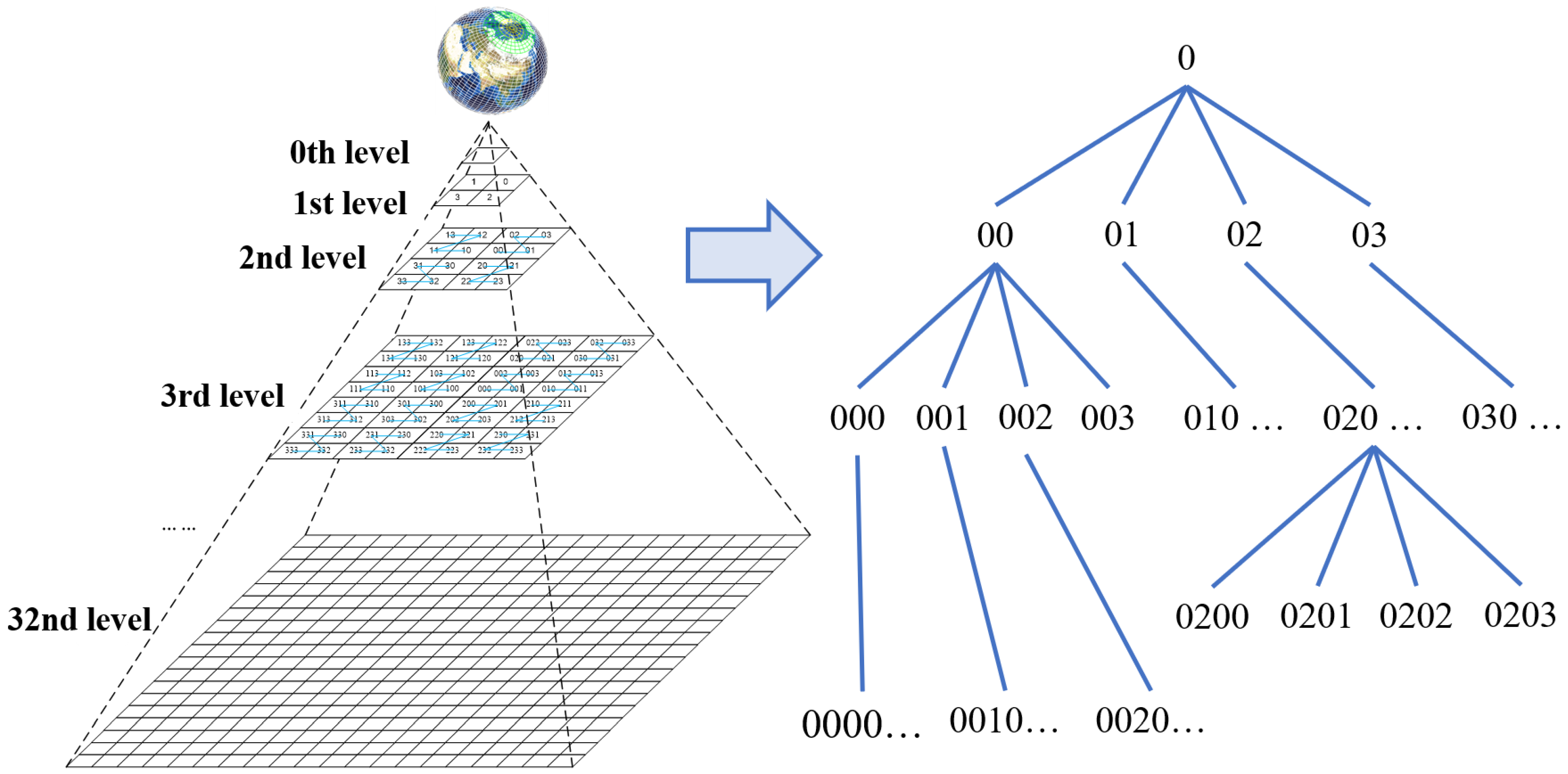
As a non-equal area grid, the GeoSOT (Geographical coordinates Subdividing grid with One dimension integral coding on 2n–Tree) grid can achieve three-dimensional expression, high efficiency of coding and calculation due to its seamless coverage of global latitude and longitude [12]. At present, it has been widely used in the fields of UAV three-dimensional spatial location identification, new postal codes, real estate codes and Beidou emergency fire big data services, and it has played a role in the compilation of international standards such as OGC, ISO, and IEEE [13,14,15].

The global hexagonal equal area grid system has been widely used in combat command, battlefield space calculation and deduction [16], etc. How to establish the information fusion and transformation of the hexagonal grid system and the standard grid system is the key problem of the two grid systems working together.

Based on the GeoSOT subdivision framework, this paper proposes the GeoSOT equivalent aggregation model (the GEA model). The GeoSOT grid is used to fit a certain scale of the hexagonal grid, and then, internal multi-scale aggregation is performed to form an encoded associative index query and finally realize the mutual transformation of information in the grid. We design the spatial association rules and information exchange model between GeoSOT grid and global hexagonal grid, and we experimentally verified its efficiency and accuracy.

2. Related Works

2.1. The GeoSOT Grid

The GeoSOT is a subdivision and coding method that discretizes the Earth’s surface with a recursive quadtree structure based on the latitude and longitude coordinate system [12] (Figure 1). Taking the intersection of the prime meridian and the equator as the center point, GeoSOT recursively divides the quadtree to form a multi-level grid system with no gaps and no overlap, and the smallest grid can reach the centimeter level. When dividing the earth’s surface into grids, the GeoSOT expands the earth’s latitude and longitude space three times (expanding the earth’s geographic space to 512°, 1° to 64′, and 1′ to 64″), so as to realize the integer quadtree dividing of integer degrees and integer minutes.

The GeoSOT code has the following characteristics [12,15]:

(1)

Consistency. GeoSOT uses the China Geodetic Coordinate System 2000 (CGCS2000) as the global space datum. In order to inherit the existing historical data to the greatest extent, GeoSOT specially retains eight grids of 4°, 2°, 1°, 2′, 1′, 2″, 1′′ and 0.5′′; these grids can be aggregated to generate the existing main standard grid.

(2)

Uniqueness. Each grid cell has a globally unique code corresponding to a rectangle on the Earth’s surface.

(3)

Recursiveness. The GeoSOT lower-level grids are divided by the upper-level grid, essentially resulting in spatial Z-order filling curve padding. The four GeoSOT grid cells of a “Z” belong to the same parent grid, and their binary codes have the same prefix.

2.2. Spherical Hexagonal Grid System

The Snyder equal area method is often used to project the subdivided icosahedron onto the surface of the sphere [17,18]. The most commonly used is the icosahedral, multi-resolution, hexagonal discrete global grid. Hexagons have a higher packing density, approximate circular regions, and each cell has equal distance from its six immediate neighbors. For spherical hexagonal grids, it can be further classified according to the aperture size of subdivided grids, where the aperture refers to the approximate area ratio of the grid cells of the upper level to those of the lower level. There are three kinds of common hexagonal grid apertures: aperture 3, aperture 4, and aperture 7 (Figure 2). Some researchers have successfully built hierarchy on several types of hexagonal bases DGGS [19,20,21]. Aperture 3 is the smallest aperture considered to have the advantage of allowing more potential grid choices. The cell directions of the aperture 4 hexagon DGGS are the same at each level, which helps to reduce the complexity of the hierarchy.

Different subdivided grids lead to different coding methods for building the grid system. For the same grid units, there are many coding methods. Common hexagonal coding methods include Hexagonal and Rhombus (HoR), Generalized Balanced Ternary (GBT) and PYXIS digital Earth reference model [21,22]. However, the use of multi-resolution, hexagon-based DGGSs has been hindered because congruent discrete grid systems cannot be constructed using hexagons. It is impossible to exactly decompose a hexagon into smaller hexagons (or, conversely, to aggregate small hexagons to form a larger one) [22]. It is difficult to make the address coding of the hexagonal grid satisfy the integrity, uniqueness and hierarchy at the same time.

3. Methods

Using the calculus thought of “many a little make a mickle”, we constructed the GeoSOT equivalent aggregation model (the GEA model). The basic unit of the global equal area grid system is the grid cell. Using the multi-scale characteristics of GeoSOT grid, the smaller-scale GeoSOT grid is regarded as a particle grid. In theory, any one equal area grid can be collectively represented. The fitting accuracy can be controlled by specifying the minimum size of the particle grid used to approximate the GeoSOT grid.

Suppose that the set A is a set of equal area grids in a certain global scale, and ${\alpha }_i$ represents equal area grid units. There are $N$ such cells under this set, $i$ is used to count the number of grids, and $j$ represents the unique identification ID of equal area grid under this system. These grid elements together constitute the global equal area grid system.

$$A={}_{i=1}{}^N\left\{{\alpha }_{i,j}\right\},$$

(1)

When using the GeoSOT grid with level $l$ as ${\beta }_{p,q}$ to approximate any cell ${\alpha }_{i,j}$, $p$ is the number of GeoSOT grids used to fit the cell, and the total number is $M_i$; $S_{{\alpha }_{i,j}}$ represents the area of cells, which is a function related to latitude and longitude; $\left(\lambda ,\theta \right)$ is the latitude and longitude of the points and edges contained in cells; and $S_{{\beta }_{p,q}}$ represents the area of each GeoSOT grid. When the grid level is high enough and the ${\beta }_{p,q}$ is small enough, the values of $S_{{\alpha }_{i,j}}$ and $S_{{\beta }_{p,q}}$ are approximately the same.

$$S_{{\alpha }_{i,j}}=f\left(\lambda ,\theta \right)=\underset{\begin{array}{c}{S}_{{\beta }_{p,l}}\to 0\\ l\to \infty \end{array}}{\lim }{\displaystyle \sum }_{p=1}^{M_i}{S}_{{\beta }_{p,l}},$$

(2)

However, the scale of the particle grid is not as fine as possible, and it is not necessary to use the particle grid for refined expression in all cases. Therefore, when using the particle grid to fit equal area grid cells, the following constraints need to be met:

(1)

The number of equal area grids used to express the study area is relatively small. Generally speaking, it needs to be controlled within 10 equal area grid cells. If the number of equal area grids is large, more information about the whole study area should be considered rather than the internal information of equal area grids.

(2)

The original point data have the characteristic of uneven spatial distribution, so it is difficult to express it finely with the large-scale equal area grid. If the spatial distribution of the internal point data in a small-scale grid is uniform, it is reasonable to extract its attribute information as the center point representation of an equal area grid.

(3)

Particle grid levels require a balance of accuracy and efficiency. With the finer scale of a particle grid, the number of grids will increase exponentially. Although the number of grids can be effectively controlled through the internal aggregation of the GEA model, the information transformation efficiency will inevitably decline, which increases the burden of data organization and management. Therefore, when selecting the particle grid level, it needs to be controlled within a reasonable scale range.

(4)

The scale of the particle grid needs to be related to the accuracy tolerance of the industry. For different industries and studies, the required minimum tolerances of precision are also different. When choosing particle grid scale, it is necessary to combine the application requirements of related industries. For example, if the education department needs to count the number of schools in a certain area, the particle grid scale can be relatively large; in the communication industry, the number of mobile terminals is huge, and the location information of the mobile terminals is constantly changing, so it is necessary to consider using the smaller grid.

(5)

The transformation method between particle grid and equal area grid is as simple as possible. Only a relatively simple transformation method can ensure that the two grids can quickly establish spatial associations.

(6)

Particle grids and equal area grids can be associated through coding, and a database can be established to achieve fast query and retrieval of data.

3.1. The Basic Definitions

3.1.1. Parent Grid and Child Grid

If the $n$-th level grid $CellA$ covers the m-th level grid $CellB (n<m)$, then $CellA$ is the parent grid of $CellB$, and $CellB$ is the child grid of $CellA$. Particularly, if $m=n+1$, then CellA is the first-level parent grid or direct parent grid of $CellB$, and $CellB$ is the first-level child grid or direct child grid of $CellA$; if $m=n+2$, $CellA$ is the second-level parent grid of $CellB$, and $CellB$ is the second-level child grid of $CellA\dots$

3.1.2. Grid Aggregation

If the $i$-th level grid $Cel{l}_i$ is all the sub-grid sets $\left\{Cel{l}_j\right\}$ at the j-th level $(i>j)$, then the grid set $\left\{Cel{l}_j\right\}$ can be aggregated into a grid $Cel{l}_i$.

3.1.3. Maximum Contained Grid

The inner region of entity O is $O^o={\cup }_{C_{rj}\subset O^o}^{j\le n_{r2}}ICel{l}_{rj}$. If $O^o$ can completely cover the $i$-th level grid $ICell$, and for any one of the $\left(i-1\right)$-th level grid $C_{i-1}$, $O^o$ is unable to completely cover $C_{i-1}$. $ICell$ is the maximum contained grid of entity $O$. There may be more than one maximum contained grid for an entity; just select one of them.

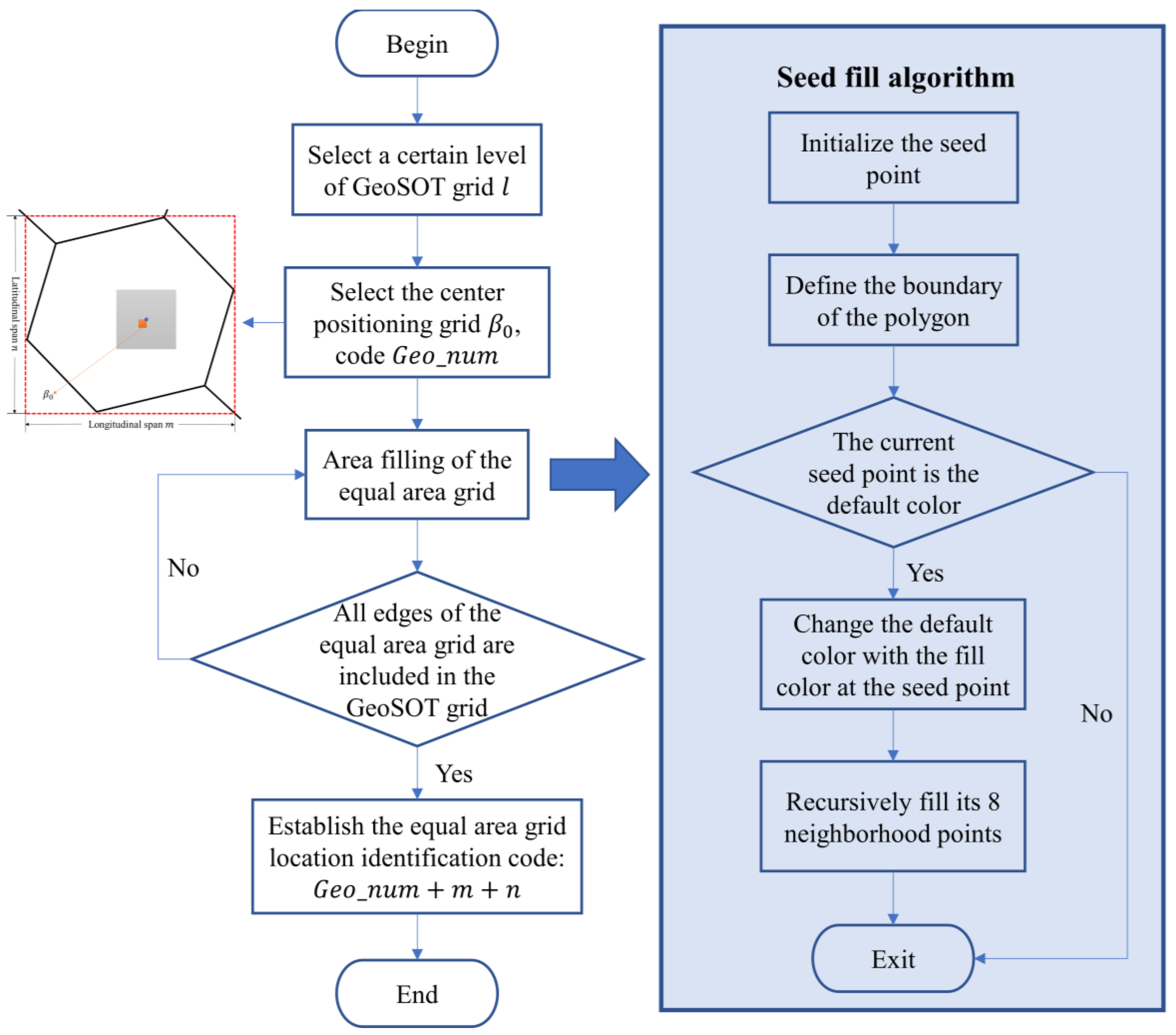
3.2. Fitting Algorithm for the Equal Area Gird

The fitting algorithm for the equal area grid is mainly composed of four parts: “select a certain level of GeoSOT grid”, “select the center positioning grid”, “area filling of the equal area grid” and “establish the equal area grid location identification code”, as shown in Figure 3.

3.2.1. Select a Certain Level of GeoSOT Grid

The smaller-scale grid of GeoSOT is the basic unit for fitting equal area grid cells, and the selection of levels affects the fitting accuracy, which is denoted as l.

3.2.2. Select the Center Positioning Grid

First, determine the maximum contained grid of the equal area grid to be fitted (if there are more than one, select the bottom-left grid), and then select the GeoSOT grid with the level l at the lower left side of the center point of the maximum contained grid, which is denoted as ${\beta }_0$.

The purpose of selecting the center positioning grid is as follows:

(1)

Based on the seed fill algorithm in computational graphics [23,24,25], the center positioning grid is used as the seed point to expand from inside to outside;

(2)

The GeoSOT grid has practical geographical meaning and can guarantee the uniqueness of the code.

3.2.3. Area Filling of the Equal Area Grid

After selecting the seed point, start to search the four neighborhoods. When all the vector edges of the equal area grid polygon are included in the GeoSOT grid, the filling is completed.

Assuming that the equal area grid cell is ${\alpha }_i$, there are $R$ vector edges ${\mu }_r \left(r=1,2, \dots , R\right)$. The searching process is to judge the grids of four neighborhoods separately, and the judgment conditions are as follows:

$${\beta }_0\cap {\mu }_r=\varnothing ,$$

(3)

If the conditions are met, continue searching, and finally ensure that any point p on ${\mu }_r$ can fall within the grid ${\beta }_i$.

$$\forall P\in {\mu }_r, P\in {\beta }_i,$$

(4)

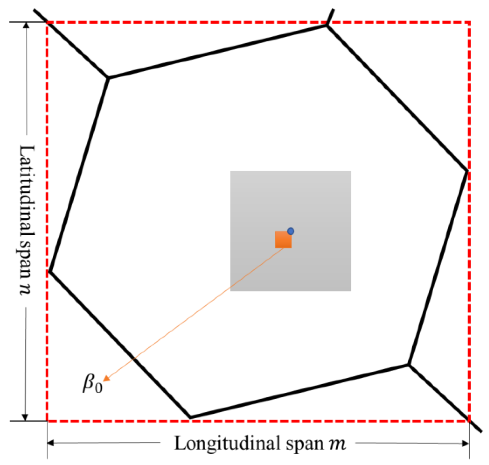
3.2.4. Establish the Equal Area Grid Location Identification Code

Referring to the method of the GeoSOT grid in real estate code identification [26], the location identification code of an equal area grid consists of three parts: the code of the center positioning grid, the longitudinal span code (the longitudinal span of the grid at the same scale level l), and the latitudinal span code (the latitudinal span of the grid at the same scale level l). Take the global hexagonal equal area grid as an example (Figure 4), the center positioning grid is ${\beta }_0$, its code is $Geo\_num$, the longitude span code is $m$, and the latitude span code is $n$.

By establishing the location identification code of an equal area grid, the equal area grid can be given a unique identification with actual geographical meaning. The identification includes the fitting scale of the GeoSOT grid, the global position of the center positioning grid, the latitude and longitude span, and other information. The location identification code has a new identification ID on the basis of the original identification ID of the equal area grid. This is an important foundation for the subsequent establishment of a relational index database.

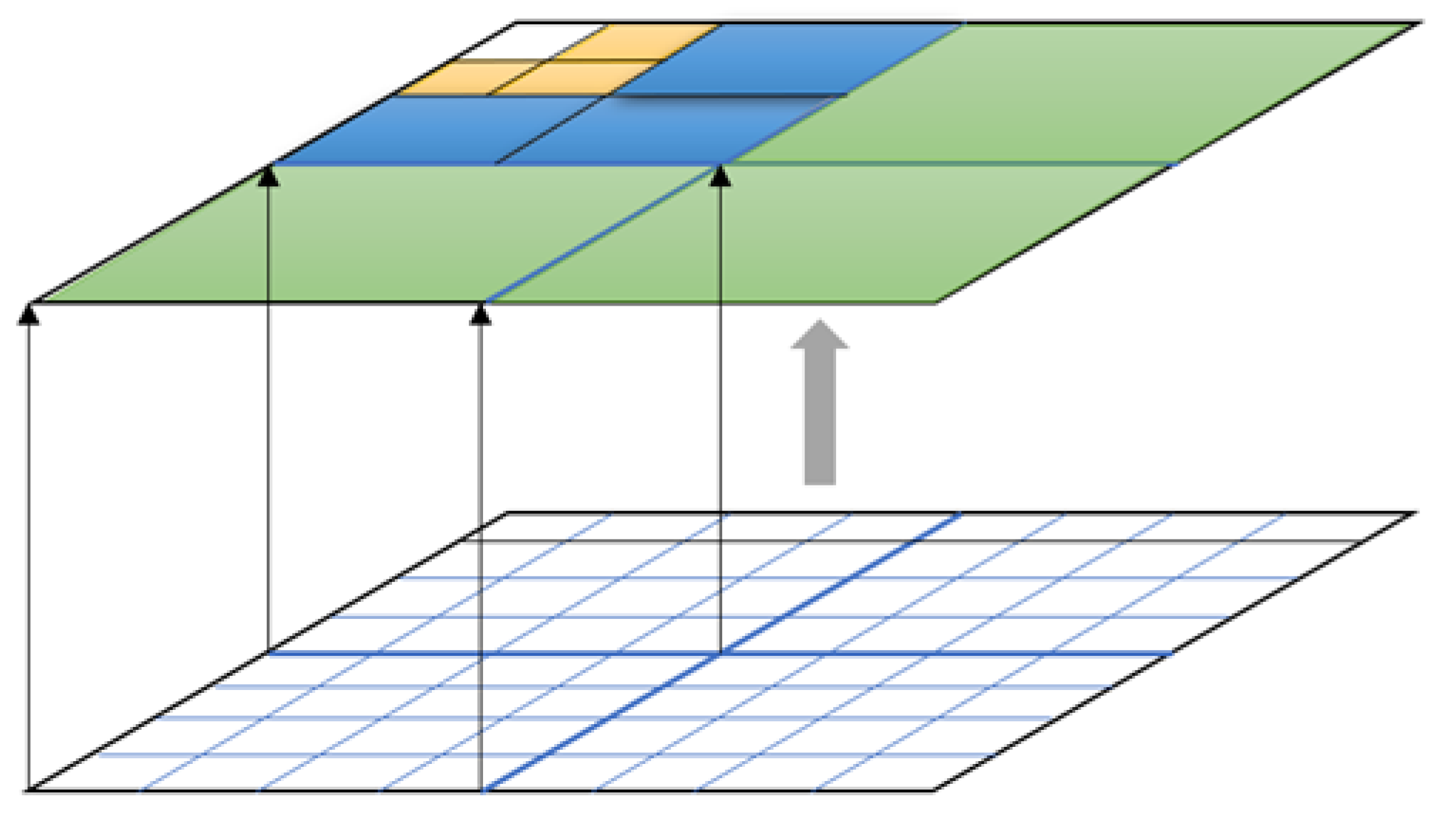
3.3. Multi-Scale Aggregation of Equal Area Grids

With the increase in the grid level, the fitting accuracy becomes higher and higher, and finally, the equal area grid approaches infinitely. However, the number of internal grids will increase exponentially, leading to data redundancy. It is necessary to construct a method that can effectively control the number of grids under the premise of ensuring the fitting accuracy. The specific solution is to internally aggregate the grids with level l up to multi-scale (Figure 5).

The fitting of a single equal area grid is sensitive to boundary information. All boundary grids with level l should be retained without affecting the overall spatial expression. The principle of multi-scale aggregation is the opposite to approximate fitting. Approximate fitting is to find seeds in the center and fill the boundary to search, while multi-scale aggregation preserves the boundary small-scale grid and aggregates from the boundary to the inside. When the maximum-scale GeoSOT grid containing the center positioning grid is generated (suppose the maximum-scale level is $\left(l-a\right)$), the aggregation stops.

The original single-scale GeoSOT grid set of approximate fitting polygons is ${\left\{\beta \right\}}_p^l$, where $p$ represents the number of grids at level l. After multi-scale aggregation, the GeoSOT grid set is:

$${\left\{\beta \right\}}_{p_1}^{l-1}+{\left\{\beta \right\}}_{p_2}^{l-2}+\cdots +{\left\{\beta \right\}}_{p_a}^{l-a}$$

(5)

where $l-i \left(i=1,2,\cdots ,a\right)$ indicates the level of the GeoSOT grid, and $p_i \left(i=1,2,\cdots ,a\right)$ indicates the number of grids at this level. The boundary grids do not participate in the aggregation, so this operation will not affect the spatial expression; that is, the area occupied by the grid sets before and after the aggregation is the same.

3.4. Establishment of Spatial Correlation Index

In Section 3.2, the equal area grids are expressed in multi-scale combination through the re-aggregation of internal small grids. The next step is to determine this spatial association by coding. Assuming that the original grid unique identifier code is $I{D}_1$, and the unique GeoSOT location identification code assigned after the aggregation operation is $I{D}_2$, which is the name of the multi-scale grid set after the equivalent aggregation model. Finally, the spatial correlation index model of “original equivalent grid code—GeoSOT location identification code—equivalent aggregation model multi-scale grid code set” is established. Figure 6 illustrates the inherent logic of spatial correlation index model by taking the hexagonal equal-area grid as an example.

4. Experiments and Results

4.1. Study Area and Data Resources

The experimental data come from the global hexagonal equal area grid provided by Jin Ben, which is a discrete grid generated by the inverse icosahedron Snyder equal area (ISEA) [22,27].

On the premise of regular grids, grids with different resolutions generated by the same subdivision method can be defined as a “grid system”. In order to quantitatively describe the relationship between grids of adjacent layers, the area ratio of units in the $k$-th layer and the $\left(k+1\right)$-th layer is defined as the “aperture” of the grid system, as follows:

$$\mathrm{aperture}=\frac{S_k}{S_{k+1}},$$

(6)

According to the size of apertures, hexagonal grid data can be divided into three types: three apertures ISEA3H (five to eight levels), four apertures ISEA4H (four to seven levels) and seven apertures ISEA7H (three to six levels).

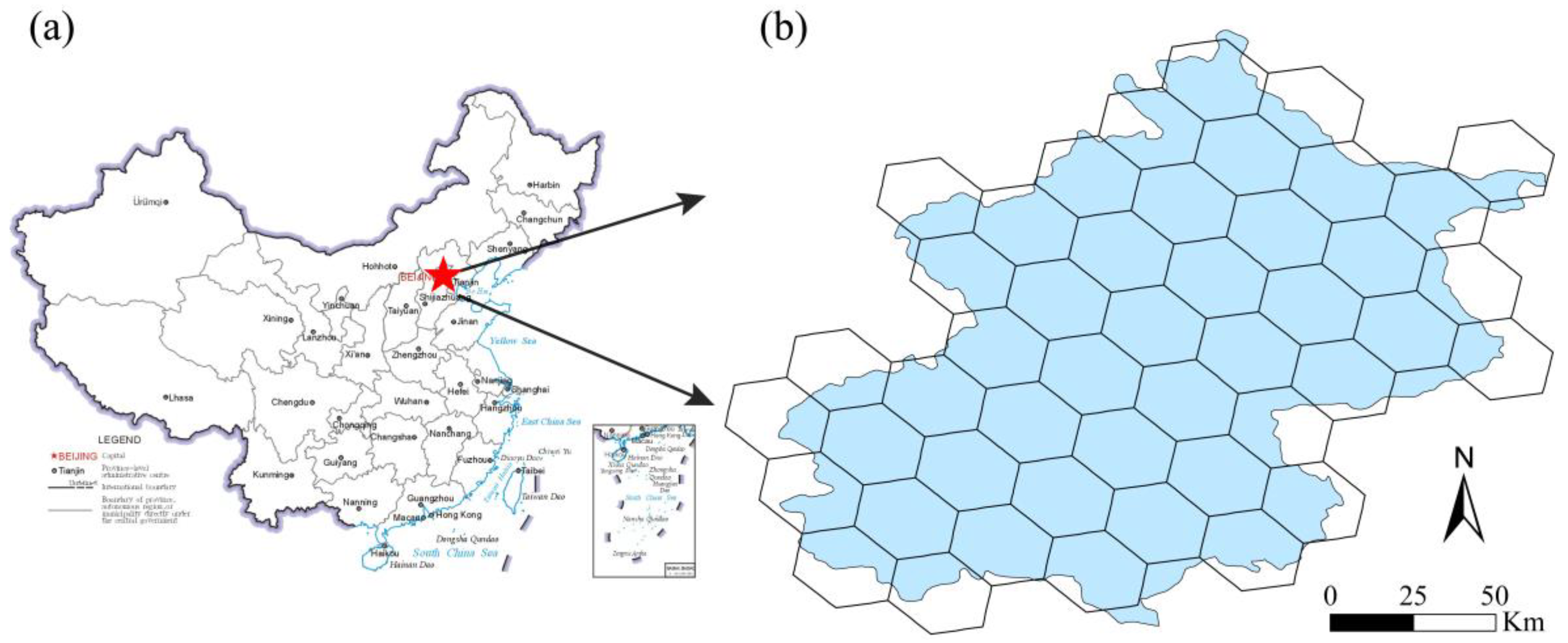
In this paper, we choose Beijing as the study area and use the 6th level hexagonal grid (ISEA7h-6) under the seven-aperture meshing method for fitting (Figure 7). Use the EPSG:4490-China Geodetic Coordinate System 2000 as the coordinate reference system for visual expression in the two-dimensional plane, and the result is shown in Figure 7b. The test data of the GEA model are the points of interest (POI) of the Beijing bus and subway stations sourced from the Baidu map (map.baidu.com) on 16 November 2021.

4.2. Transformation from Hexagonal Grid to GeoSOT Grid

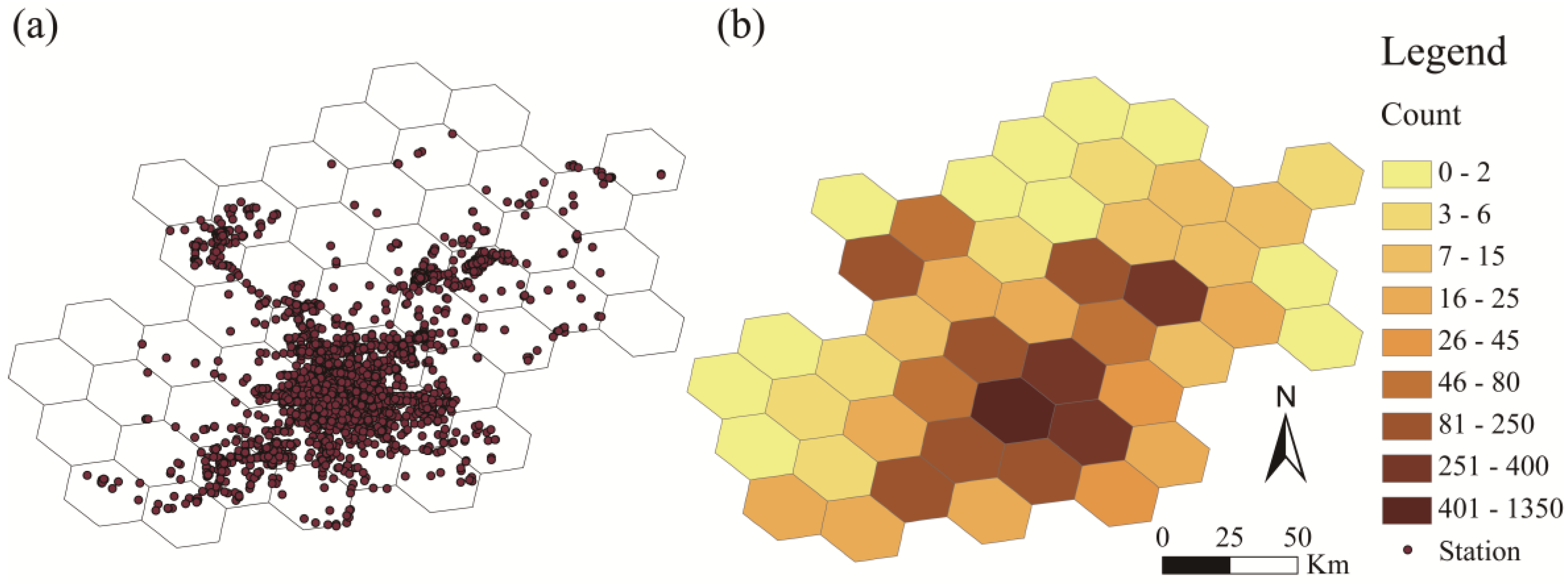
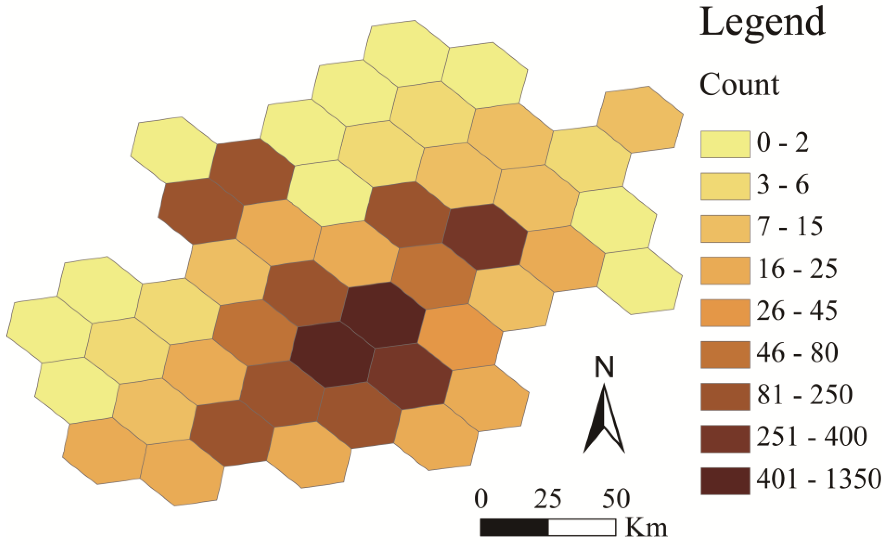
Firstly, a hexagonal grid (ISEA7h-6) is used to organize the POI data, the number of points in the grid is used as the attribute of the grid, and a heat map of the distribution of public transportation stations in Beijing is generated (Figure 8).

Secondly, we express the attribute information of the hexagon by the center point; then, we find the GeoSOT grid of the adjacent level (level 11) of the hexagon grid and obtain its center point. Then, the inverse distance weighting method (IDW) is used for interpolation and resampling to obtain a heat map of the distribution of public transportation stations in Beijing (Figure 9).

Finally, we compare the resampled spatial interpolation result with the true value of the POI data in the GeoSOT grid. The evaluation index adopts the coefficient of determination $R^2$, and it can be given by:

$$R^2=1-\frac{SSE}{SST}=1-\frac{\sum {\left(y_i-{\widehat{y}}_i\right)}^2}{\sum {\left(y_i-\overline{y}\right)}^2},$$

(7)

For the $i$-th observation point, the difference between the $y_i$ of the real data and the estimated ${\widehat{y}}_i$ is called the $i$-th residual, SSE represents the sum of squares due to error; and SST represents the total sum of squares. The closer the value of $R^2$ is to 1, the stronger the explanatory power of the variables of the equation to $y$, and the better the model fits to the data.

The accuracy evaluation index of the GEA model for information transformation can be written as:

$$Accuracy=1-MAPE=1-\frac{1}{n}{\sum }_{i=1}^n\frac{\left|y_i-{\widehat{y}}_i\right|}{y_i}\times 100\%,$$

(8)

The calculated value of $R^2$ is 0.90575, indicating that the fitting result of the spatial interpolation model is reasonable. However, the transformation accuracy from hexagonal grid to GeoSOT grid is 72.51%, which indicates that the average relative error between the interpolation result and the true value is relatively large under similar scales. In the process of converting the attribute information of the hexagonal grid to the GeoSOT grid, select a GeoSOT grid with a similar scale to the hexagonal grid, and resample through the spatial interpolation method. This method has certain feasibility, but the fitting is obtained The attribute information of is not accurate enough.

4.3. Transformation from GeoSOT Grid to Hexagonal Grid

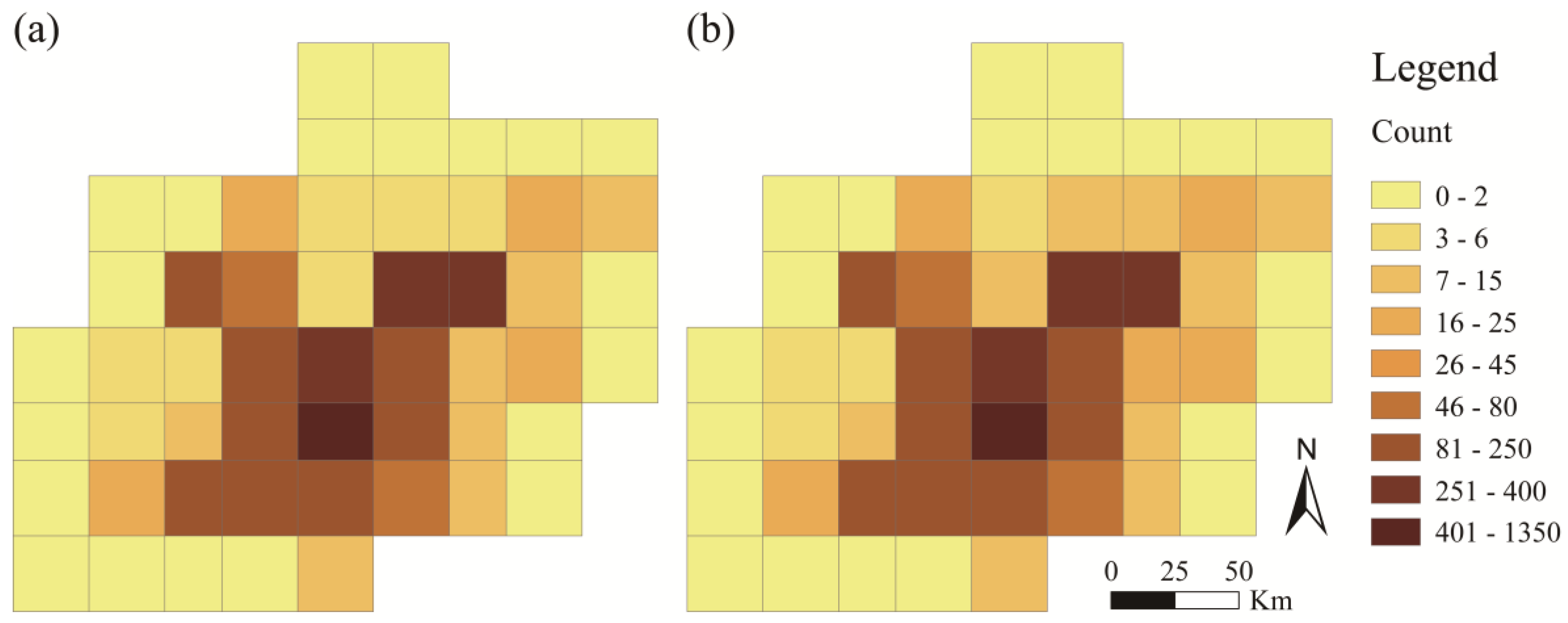
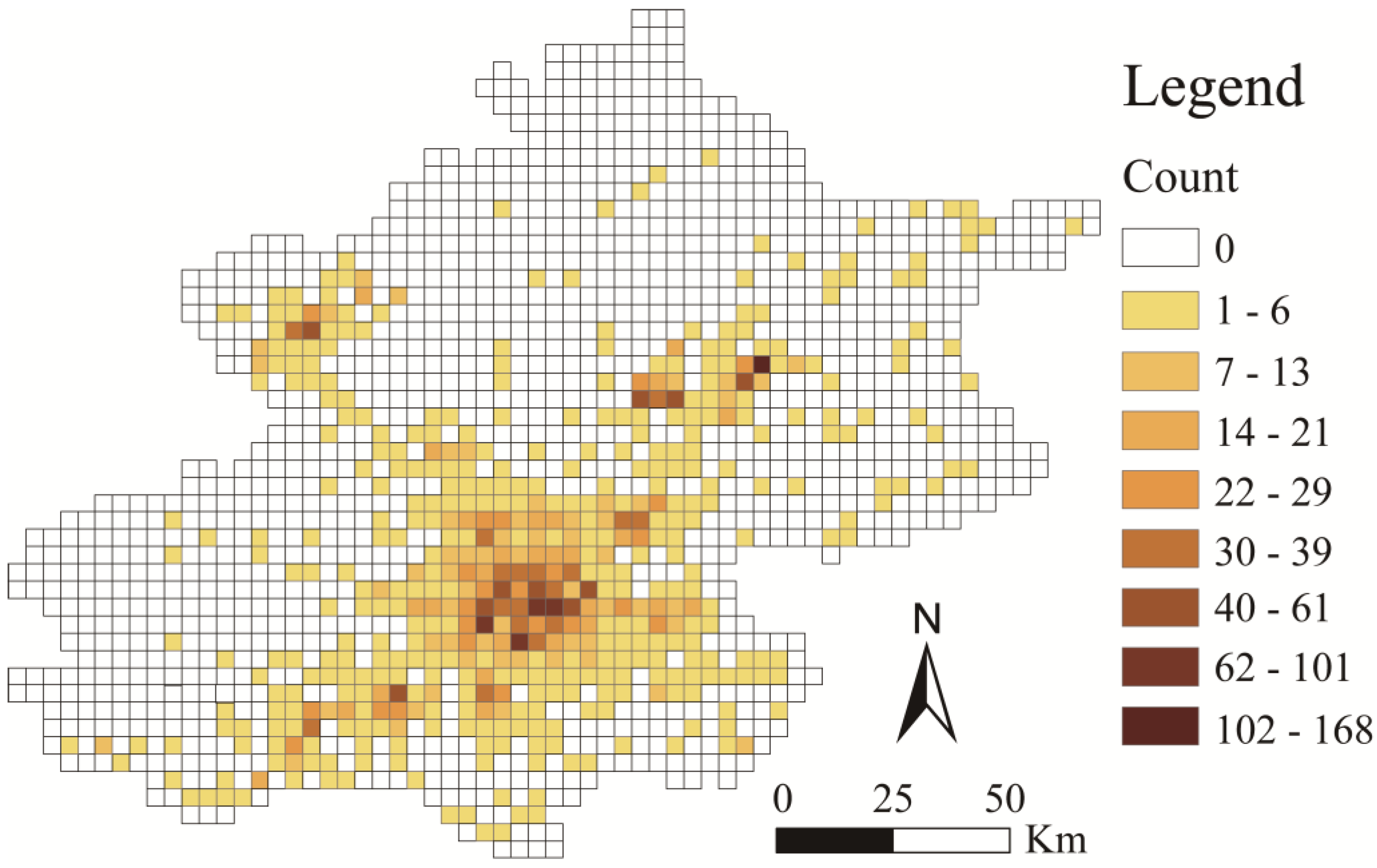
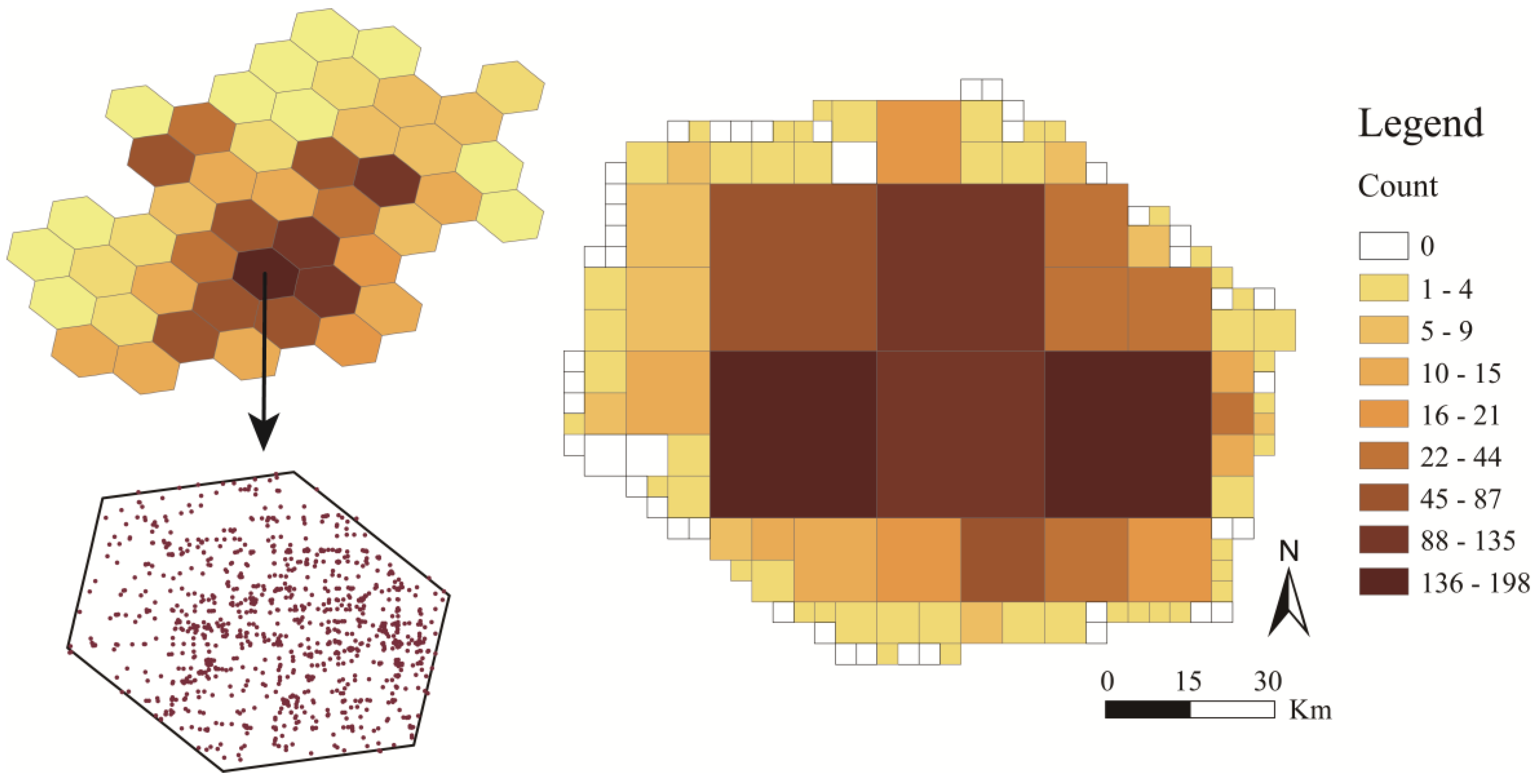
Firstly, we use a relatively small-scale GeoSOT grid (take the 14th level as an example) to fit each hexagonal grid to obtain the GeoSOT particle grid set of the study area.

Then, we use particle GeoSOT grids to organize the POI data, take the number of points in the grid as the attributes of the grid, and generate a heat map of the distribution of public transportation stations in Beijing (Figure 10).

Finally, we gather the attribute information contained in the GeoSOT particle grid upwards into a hexagonal grid, and we obtain the heat map expressed by the hexagonal grid after information transformation (Figure 11).

Taking the GeoSOT grid as the baseline, we calculated the accuracy and efficiency of the information transformation for the GeoSOT grid and the GEA model at different levels of particle grids. The results are shown in

Table 1. Accuracy and efficiency of particle grids at different levels for GeoSOT and the GEA model.

Level of Particle Grid		14	15	16	17	18
	GeoSOT	55.54	71.42	81.88	85.96	92.79
Fitting accuracy (%)	The GEA model	69.42	84.02	90.98	95.51	97.67
	GeoSOT	0.9	1.9	21.7	29.3	110.9
Run time (ms)	The GEA model	0.9	2.0	22.9	30.9	116.7

.

As the level of the particle grid increases, the accuracy of information transformation becomes higher and higher, but the transformation time will also increase. It can be seen from the table that when the 17-level GeoSOT grid is selected as the particle grid, the accuracy and efficiency can be better balanced. In the process of transforming the attribute information from GeoSOT grid to hexagonal grid, adopting the GeoSOT equivalent aggregation model of appropriate scale can realize the accurate transformation of attribute information under the premise of ensuring time efficiency.

4.4. Spatial Correlation Index of GeoSOT Grid and Hexagonal Grid

For a hexagonal grid with a high density of point data, it is difficult for a single-scale particle grid to accurately obtain internal information. Use the grid collection obtained by GeoSOT multi-scale grid aggregation, and then establish a spatial correlation index with the hexagonal grid (Figure 12), and establish a database (Figure 13).

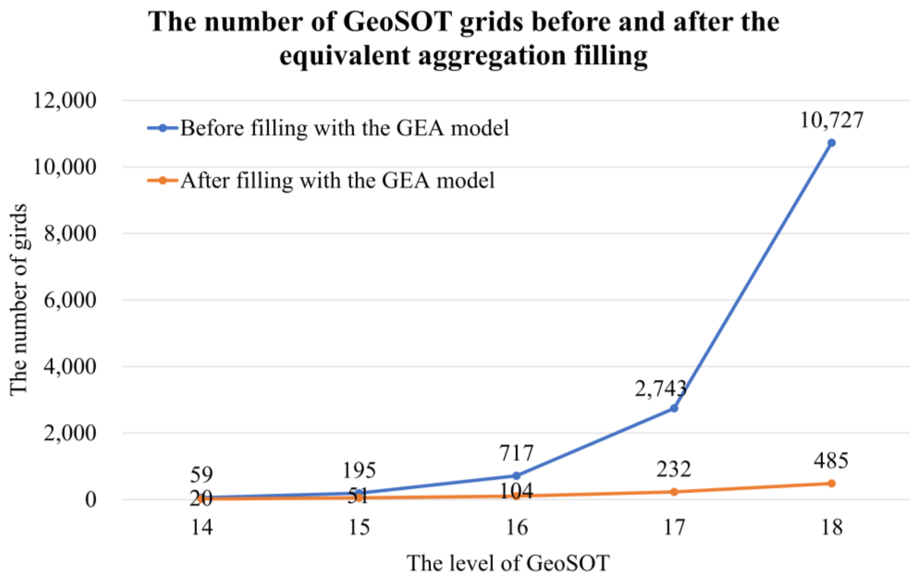
According to the particle small grid filling and equivalent aggregation filling of each hexagonal grid, we obtain the comparison of the number of GeoSOT grids before and after the equivalent aggregation filling (Figure 14).

As the level of particle grids increases, the number of particle grids required to fill the hexagonal grid will increase sharply. However, the number of grids can be effectively controlled through equivalent aggregation and filling. By aggregating particle grids, it is possible to greatly reduce the number of grids in the associated index table, improving the efficiency of data organization and management. Thus, we can achieve a multi-scale expression of spatial information without affecting the spatial expression and attribute information transformation.

5. Discussion

In this paper, the multi-scale characteristics of GeoSOT grids are used to fit hexagonal equal area grids. We first determine the minimum grid size and find the center positioning grid. Then, we obtain a small-scale grid set according to the method similar to regional seed fill algorithm, and we obtain the location identification code. The GEA model re-aggregates the interior of the small-scale grid to obtain the multi-scale representation of the equal area grid, which greatly reduces the number of grids.

We use the GEA model proposed in this paper to fit the real data of the hexagonal grid and demonstrate that the GEA model can effectively reduce the number of particle grids. By aggregating particle grids, the GEA model can greatly reduce the number of grids in the associated index table without affecting the spatial expression and attribute information transformation, improve the efficiency of data organization and management, and achieve multi-scale expression of spatial information. In addition, we analyze and compare the accuracy and efficiency of particle mesh fitting at different levels, and we obtain the optimal hierarchical particle mesh that balances efficiency and accuracy. Here, the model is scientifically demonstrated from the perspective of global uniqueness, multi-scale and efficient data organization.

5.1. Uniqueness

For any global equal area grid, the GEA model can find a unique center positioning grid, thereby generating a unique location identification code.

5.2. Multiscale

The global hexagonal equal area grid is limited by the spatial division rules, and it is difficult to achieve seamless global multi-scale subdivision without overlapping. However, the use of the global multi-scale feature of GeoSOT grid can just make up for this shortcoming of equal area grid. Through the spatial correlation index model, the GeoSOT grid can be used as the basic unit of information collection. If we need to know the fine-scale information inside the hexagonal grid, we can quickly find it through the spatial correlation index model. On the contrary, if an attribute change occurs in a GeoSOT grid, the change information can be aggregated into the hexagonal grid simultaneously through the spatial correlation index model.

5.3. Efficient

The GeoSOT grid has high efficiency of coding calculation. On this basis, the GEA model proposed in this paper greatly reduces the number of grids of the same scale through internal aggregation and effectively controls the total number of grids without affecting the overall spatial expression, thus improving the efficiency of data organization and management.

6. Conclusions

In order to solve the problem of lack of unified rules between a GeoSOT grid and hexagonal grid, this paper proposes a GeoSOT grid and hexagonal equal area grid information fusion transformation model. It solves the difficulty of cooperating with major DGGS and provides a new idea for cross-system grid information fusion. Using the multi-scale characteristics of GeoSOT grids, we established a spatial correlation index of “Hexagonal grid code–GeoSOT unique location identification code–GeoSOT multi-scale grid code set”. The GeoSOT grid is used as the base for data collection, organization and management, and it is aggregated upward into the equal area grid for spatial calculation of the equal area grid. Based on the GEA model, we carried out the hexagonal grid to GeoSOT grid information transformation experiment. Finally, we demonstrated the advantages of the GeoSOT equivalent aggregation model in controlling the number of fitted grids and multi-scale expression.