An Efficient Plane-Segmentation Method for Indoor Point Clouds Based on Countability of Saliency Directions

Abstract

This paper proposes an efficient approach for the plane segmentation of indoor and corridor scenes. Specifically, the proposed method first uses voxels to pre-segment the scene and establishes the topological relationship between neighboring voxels. The voxel normal vectors are projected onto the surface of a Gaussian sphere based on the corresponding directions to achieve fast plane grouping using a variant of the K-means approach. To improve the segmentation integration, we propose releasing the points from the specified voxels and establishing second-order relationships between different primitives. We then introduce a global energy-optimization strategy that considers the unity and pairwise potentials while including high-order sequences to improve the over-segmentation problem. Three benchmark methods are introduced to evaluate the properties of the proposed approach by using the ISPRS benchmark datasets and self-collected in-house. The results of our experiments and the comparisons indicate that the proposed method can return reliable segmentation with precision over 72% even with the low-cost sensor, and provide the best performances in terms of the precision and recall rate compared to the benchmark methods.

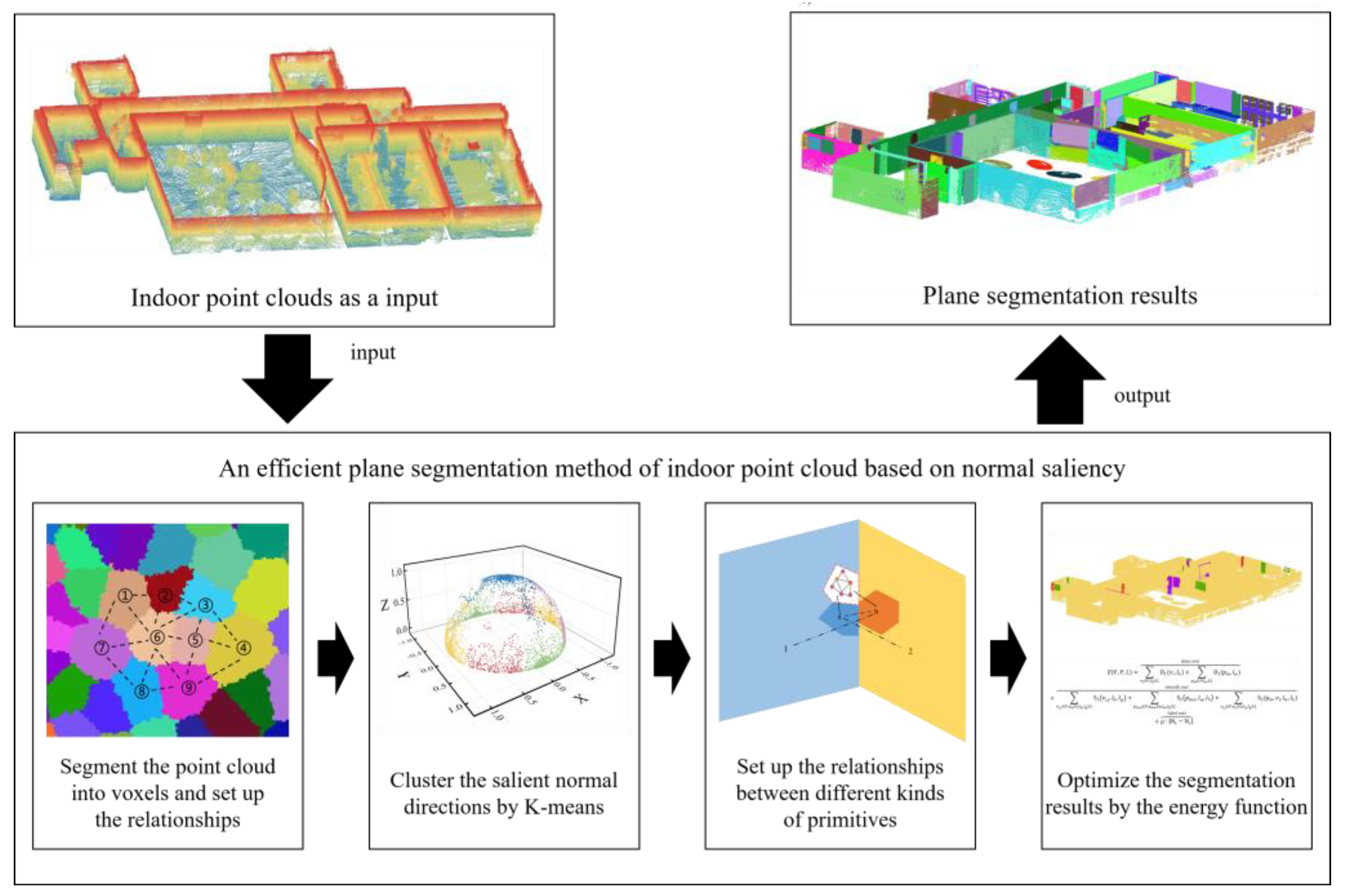
1. Introduction

The reconstruction of 3D indoor scenes, e.g., indoor navigation, construction completion acceptance, and interior design, has received increasing attention. As the physical geometry of buildings often differs from its original plan, reconstructing a real 3D model for building interiors is a common need. Considering that indoor environments contain several planar structures, 3D plane segmentation remains a suitable choice for 3D-scene reconstruction [1,2]. In artificial buildings, planar structures regularly adapt to one of the following relationships: parallelism, orthogonality, coplanarity, and angular equality. Appropriate use of these geometric characteristics can significantly improve the accuracy and robustness of indoor 3D plane segmentation; however, few methods have introduced prior information to constrain the adjustments. Traditional plane-extraction methods (e.g., region growing (RG) [3], Hough transform (HT) [4]) do not take advantage of these geometric characteristics but rely heavily on the point-cloud quality. Although the random-sample consensus (RANSAC) [5] allows us to introduce such structural information, it is very sensitive to the parameters that are set. Thus, high-noise sensors, such as low-cost RGB-D sensors [6,7], that are popular for indoor applications are not suitable for classic approaches.

This paper develops a fast and robust approach oriented toward indoor 3D plane segmentation. Unlike traditional strategies, our approach reconstructs surfaces with the saliency of normal directions. There are two main steps in the proposed method. First, we perform spatial segmentation based on the saliency analysis of the normal directions. The spatial structures are then quickly cut into finite planes. Second, we drive the high-order energy model to optimize the segmentation based on the multi-level topologic relationships. This step improves the robustness and reduces the risk of over-segmentation.

Three major contributions of the proposed method are described as follows:

(1) The method introduces the countable of main normal directions in an enclosed space favor to rapidly cluster surfaces.

(2) The method develops multi-level topological relationships with three primitives from different stages and designs a high-order cost–energy model for indoor cases to optimize the segmentation and improve the accuracy and robustness.

(3) The obtained precise 3D model sundries in houses are automatically removed to the greatest extent; thus, our method generates a precise indoor 3D model for construction sites.

2. Related Works

Point-cloud segmentation has been studied and explored for decades. Research can be roughly divided into four categories: model fitting, RG, feature clustering, and global energy-optimization methods. This section briefly reviews works immediately related to plane segmentation.

Model-Fitting-Based Methods. The RANSAC [5] and HT [4] are common fitting-based methods [8] that use known geometric primitive shapes (sphere, cone, plane, and cylinder) to segment point-cloud data. Point clouds with the same mathematical representations are grouped as the same object. Researchers recently improved the performance of RANSAC in terms of robustness and efficiency. For example, Li et al. [9] proposed an improved RANSAC method based on normal-distribution transformation cells to avoid spurious planes (over-segmentation) for plane segmentation. Hamid-Lakzaeian [10] proposed the Gridded-RANSAC method, which uses grid concepts to organize inherently unorganized datasets to speed up the segmentation. Lina et al. [11] proposed to use normal vectors to accelerate RANSAC to extract planes from point clouds. To accelerate the calculation speed and further increase the reliability of the HT algorithm, Tian et al. [12] proposed a novel method to segment planar features from unorganized point clouds based on a 2D HT and octree.

Although the RANSAC and HT have been widely used in segmentation tasks, these approaches have inherent shortcomings. First, they are both sensitive to the parameter selection for segment-based modeling. Although many studies have focused on various point-cloud densities, it is still difficult to attain a real self-adaption method. Moreover, RANSAC is suitable for point-cloud data with small data volumes and less surface geometric information; otherwise, the algorithm performance is poor [13]. The key shortcomings of the HT method are the time and/or space complexities, which limit its applicability. Many authors [14] compared the HT and RANSAC and showed that the HT is less efficient in computational time when fit to large datasets. Compared with RANSAC and HT, the proposed approach does not require setting many parameters, indicating it is not sensitive to the parameter choice.

Region-Growing-Based Methods. RG-based methods usually select a seed and generate the seed surface. This surface is then used as the starting region, and the similarities of each point in the neighborhood are compared to the seed surface in order to group discrete point clouds around each seed surface. These continually expand outward until finally achieving complete segmentation. Depending on the algorithm principle, this method must acquire adjacent points and calculate the associated characteristic information, which leads to low computational efficiencies. Anh-VuVo et al. [13] used the RG algorithm to roughly segment the octree-based voxelized representation of the input point cloud to accelerate the calculations. However, restricting the handing process using specific growth rules cannot readily meet the attributes of all the primitives contained in the data; therefore, improvements to the efficiency are not obvious. In addition, the results from the RG are affected by the initial seed-surface selection, while an improper selection readily causes significant segmentation errors. Many scholars have focused on improving the accuracy of this approach. For example, Luo et al. [15] proposed a super-voxel-based point-cloud-segmentation algorithm that improves the inaccurate boundaries and unsmooth segmentation in existing methods. One of the differences between the proposed method and the RG method is that it does not need to judge normals individually, which overcomes the efficiency bottleneck.

Feature-Clustering-Based Methods. Feature-clustering-based methods primarily use the geometric-structure features or spatial-distribution features of point clouds to cluster them and obtain segmentations. Holz et al. [16] realized the real-time plane segmentation of point clouds using the surface normal vector, which can perceive salient target objects in point-cloud scenes in real-time. Wu et al. [17] proposed a smooth-Euclidean-clustering segmentation approach based on the traditional Euclidean-clustering algorithm. This prevents over- or under-segmentation by adding the constraint of a smoothing threshold. Feature-clustering-based methods are flexible in terms of feature selection. Specific features can be selected based on differences between point clouds, which gives it a high accuracy. However, this method has certain requirements for neighborhood definitions and is sensitive to noise [18]. In addition, it is highly dependent on features, indicating that the quality of feature selection significantly impacts the final segmentation effect. However, the greater dimensionality of a feature yields a lower calculation efficiency. In contrast, our approach introduces a predetermined parameter based on prior knowledge for a more efficient and robust approach. Currently, with deep-learning methods being widely introduced to handle point clouds, many researchers have proposed to use neural networks to segment point clouds [19] and further implement 3D reconstruction [20]. One benefit of the high-order feature learning is that the network always has a good adaptability. Many networks can handle imperfect data, e.g., noise [21], and some of them have the potential to repair the shapes, e.g., the GANs [22]. However, most neural networks benefit from a large number of labeling samples; namely, the samples heavily constrain the performances of learning-based methods.

Global Energy-Optimization-Based Methods. Global energy-optimization-based methods formulate plane segmentation as an energy-optimization problem. Pham et al. [23] expressed plane-extraction tasks as a global energy function that forces the extracted planes to be orthogonal or parallel to each other in order to robustly find underlying planes in a scene. Dong et al. [24] linked all voxels and established rules between them to calculate the overall energy. They then used graph theory to apply the graph cut and attain the minimum energy state. Lin et al. [2] applied L0 gradient minimization to plane fitting in order to contain a high proportion of noise and outliers. Compared with other methods, energy optimization can better handle data with high noise levels [25]; however, this method requires significant calculations when performing plane segmentation and most require initial segmentation results [25]. Thus, the proposed approach establishes the relationships for the primitives, makes the rules, and optimizes the interaction to influence the segmentation results.

3. Methodology

3.1. Motivation

As human-made buildings have strong structural constraints, a typical constraint is the Manhattan world model [26], which is among the popular hypothetical models to segment and reconstruct indoor spaces. The Manhattan world model states that all surfaces in the world are aligned with three dominant directions, typically corresponding to the X-, Y-, and Z-axes; that is, the world is piecewise axis-aligned and planar. Remarkably, the original Manhattan world model is not suited to complex structures, so the constraint has developed into the multi-Manhattan world model. The lack of angular constraints is the primary shortcoming of the Manhattan and multi-Manhattan world models. Thus, Monszpart et al. [26] introduced angular constraints and derived the general Manhattan world model, and Lin et al. [27] proposed a directional constraint model based on the directions of normal vectors. Inspired by these constraint models and combined with the characteristics of indoor scenes (directions of normal vectors can be exhausted), we propose segmenting point clouds into countable clusters based on the saliency analysis of the directions. We define a saliency direction as gathering at least more than 5% of points in a sample cluster. To introduce the proposed approach, we first give the overall workflow of our method in Figure 1.

3.2. Super-Voxel-Based Segmentation and Topological Relationships

Whether indoor laser scanning, image dense matching, or SLAM, existing indoor point-cloud-acquisition methods can obtain dense and highly redundant point-cloud data, which makes data processing time-consuming. Therefore, we first segment point clouds using super voxels, i.e., contain the properties in a voxel, in order to accelerate the following processes. Our experiments employed the voxel-based-segmentation method described by Lin et al. [22]. We set the resolution of the voxel to $\sigma =0.2 \mathrm{m}$ to maintain more details of the objects in indoor scenes. This also guarantees that points in the same voxel have as similar properties as possible. A resolution setting that is too small, e.g., centimeter level, creates significantly fragmented information. One of the main advantages of Lin’s method is that the voxels can limit crossing object boundaries. Remarkably, this effect significantly improves the normal directions of voxels that are close to boundaries. The normal vector ${\overrightarrow{\mathrm{n}}}_v$ of voxel v is calculated from the normal vector of the point set ${\mathrm{S}}_v$ (i.e., the point i ∈ ${\mathrm{S}}_v$ and the corresponding normal vector is ${\mathit{normal}}_i$) contained in v as,

$${\overrightarrow{\mathrm{n}}}_v=\frac{1}{n}{\displaystyle \sum }_{i\in n}norma{l}_i.$$

(1)

Based on super-voxel segmentation, we establish the topological relationship between voxels that support subsequent instances and global optimization. The topological relationship between voxels is represented by ${\mathsf{\rho }}_v$. We form a linked topological relationship between two voxels based on their adjacency. Figure 2 shows the voxels along two different types of walls with partially linking topological relationships. For example, the No. 6 voxel in the left graph has the ${\mathsf{\rho }}_v=\left\{⑥|①,②,③,⑤,⑦,⑧,⑨\right\}$ relationships. The spatial position ${\mathrm{v}}_{x,y,z}$ of voxel v is represented by the spatial coordinates of the center position of ${\mathrm{S}}_v$. Subsequently, the description-feature vector ${\mathrm{N}}_v$ of the voxel is obtained as

$${\mathrm{N}}_v=({\overrightarrow{\mathrm{n}}}_v,{\mathsf{\rho }}_v,{\mathrm{v}}_{x,y,z})$$

(2)

3.3. Directional Saliency Analysis in Indoor Environments

The normal vector ${\mathrm{N}}_v$ of voxel v can be projected onto the Gaussian half sphere for statistics. Intuitively, the normal vector has a significant aggregation effect, and each cluster reflects a salient direction, as seen in Figure 3a. Statistical strategies can readily remove outliers on the Gaussian half-sphere, which are represented as hollow dots in the figure. To improve the description and understanding, a voxel v that is judged to be an outlier is denoted as $v^{\prime }$.

We deem that the number of normal directions in indoor scenes is limited. Thus, we employ a clustering approach to increase this number and further segment the space. We use the mini-batch K-means [28] approach to divide the normal direction sets, which are a convex dataset, into K classes. The bias between a point to the clustering center primarily results from the random errors in the observations. Thus, these biases $\mathsf{\epsilon }$ in terms of one clustering center present a normal distribution $\mathcal{N}$ with the standard deviation ${\sigma }_0$ as,

$$\mathrm{E}\left(\mathsf{\epsilon }\right)=0, \mathsf{\epsilon }~\mathcal{N}\left(0,{\sigma }_0^2\right).$$

(3)

This property can benefit from K-means methods to attain perfect results. To start the K-means process, we approximately set K = 30 and then iterate a reasonable constant $\hat{\mathrm{K}}$. The threshold K is generated from the cognitions and experiences of indoor scenes [2].

Figure 3b displays the processed results of the K-means clustering on the Gaussian half-sphere (note: the different colors in Figure 3b,c represent different clusters). The normal direction of the two super voxels on opposite planes appear as ${\overrightarrow{\mathrm{n}}}_1=-({\overrightarrow{\mathrm{n}}}_2)$ because we set the viewpoint in the room. Therefore, we further reduced the number of normal directions, as seen in Figure 3c. Figure 4 illustrates segmentation in an indoor space using the saliency normal directions. Some mistakes are seen in the segmentation, such as the green points on the door, which should be red. The dividing line of the two clusters is unclear; thus, the results from the K-means are not always optimal. However, we can eliminate nearly all these errors in subsequent global optimization strategies. To facilitate subsequent processing (regularization and reconstruction), we performed instance segmentation using the voxel-based topological relationships, as seen in Figure 5.

Two special cases should be considered in the instance segmentation that easily cause under-segmentation issues. This includes (I) two parallel planes being very close to each other and (II) a lack of discrimination in the differences between two normal directions. Figure 6a shows the first situation, where the pseudo-connection relationship between voxels is caused when either the distance d between two planes is less than the given threshold ${\epsilon }_d$ (=2.5 times point density in our cases) or there are noise points between the two planes. The second issue is displayed in Figure 6c, where the angular difference of two normal directions is not significant in the K-means processing. To address these problems, we further fit planes for each cluster with a more stringent planeness, $f_d<0.5{\epsilon }_d$. Figure 6b,d show two related examples before and after processing. The validation process is performed in parallel as each of the w trials (handles one of the clusters) is independent of the others, which gives a straightforward processing increase. Our implementation used the OpenMP application programming interface to distribute separate trials and check different threads.

3.4. Global Energy Optimization

There are substantial noise points in point clouds. Although strategies for voxel-based and saliency normal directions can improve the robustness of data processing, some voxels inevitably contain corners and boundary points that significantly reduce the accuracy of normal estimations [29]. This section handles such outliers as the global energy-optimization problem. The ground-truth segmentation was defined as the optimal energy state, i.e., E = 0. We then defined different rules to judge and penalize the relationships between primitives. We finally introduced the graph cut [30] to calculate the optimal segmentation results.

3.4.1. Outlier Voxels

There are many outlier voxels in real datasets, which are shown as the hollow dots in Figure 3a. We can distinguish these outliers into two categories. One is that a voxel’s normal direction is significantly different from those of their neighbors and the other is “ghost” voxels. For segmentation purposes, we need to repair the first type of outliers and prune the second type. As the first type of outliers are caused by noise and corner edges, there are many useful points in such voxels that do not need to be directly removed.

3.4.2. Relationship between Different Primitives

We established a graph to connect all the primitives based on the topologic relationships [31]. The voxel acts as the main primitive, and the associated primitive-relationship network was described in the previous section. Therefore, this section enriches and completes the relationship network by introducing other primitive types (plane and point primitives). We first established the connections between voxels and their corresponding plane, released the points from the first type of outlier voxel, and constructed the point-to-point and point-to-voxel links. Figure 7 shows a schematic diagram of the multi-level relationships for the primitives. Edges that connect two primitives not only represent the topologic relationships but also express interactions between primitives. Such forces have both magnitude and directionality, which reasonably suggests that the effects are closely related to the primitive type. Compared with the voxel primitive, the plane primitive has more deterministic properties; however, the point primitive is the opposite.

3.4.3. Energy Function Formulation

We treat the segmentation-optimization problem as labeling optimization with a global energy function [24] in order to balance the geometric errors, spatial consistency, and high-order potentials. Thus, we establish the energy function as,

$$\begin{gathered} E(V,P,L)=\stackrel{data cost}{\overbrace{{\displaystyle \sum }_{v_i\in V;l_k\in L}{\mathrm{D}}_1\left(v_i,l_k\right)+{\displaystyle \sum }_{p_m\in P;l_w\in L}{\mathrm{D}}_2\left(p_m,l_w\right)}} \\ +\stackrel{smooth cost}{\overbrace{{\displaystyle \sum }_{v_{i,j}\in V;e_{ij}\in e;l_k,l_g\in L}{\mathrm{S}}_1\left(v_{i,j},l_k,l_g\right)+{\displaystyle \sum }_{p_{m,n}\in P;e_{mn}\in e;l_w,l_h\in L}{\mathrm{S}}_2\left(p_{m,n},l_w,l_h\right)+{\displaystyle \sum }_{v_{i,j}\in V;e_{ij}\in e;l_k,l_g\in L}{\mathrm{S}}_3\left(p_m,v_i,l_w,l_k\right)}} \\ +\stackrel{label cost}{\overbrace{\mu ·\left|{\mathrm{N}}_L-{\mathrm{N}}_c\right|}} \end{gathered}$$

(4)

where ${\mathrm{D}}_1$ and ${\mathrm{D}}_2$ represent the data-cost measure as the sum of geometric errors from the voxel and point primitives, respectively; ${\mathrm{S}}_1$, ${\mathrm{S}}_2$, and ${\mathrm{S}}_3$ are the smooth-cost terms that penalize the label inconsistency between connected primitives (voxel–voxel, point–point, and point–voxel); and $\mu ·\left|{\mathrm{N}}_L-{\mathrm{N}}_c\right|$ represents the high-order potentials related to the number of labels ${\mathrm{N}}_L$, which is the so-called label cost. The data-cost term ${\mathrm{D}}_1\left(v_i,l_k\right)$ represents the potentials of voxel $v_i$, with the label $l_k$. According to the principle of the proposed method, $v_i$ belongs to the plane labeled as $l_k$; otherwise, it is removed or released. We calculate the potentials for ${\mathrm{D}}_1$ with a Gaussian kernel function as,

$${\mathrm{D}}_1\left(v_i,l_k\right)=\{\begin{array}{c}\begin{array}{cc}\ln \left(\mathsf{\alpha }·\exp \left(\frac{{\mathrm{M}}_{\mathrm{dis}}{\left(p,l\right)}^2}{2·{\sigma }^2}\right)\right),& l=l_k\end{array}\\ \begin{array}{cc}2\sigma ,& l\ne l_k\end{array}\end{array},$$

(5)

where ${\mathrm{M}}_{\mathrm{dis}}\left(p,l_k\right)$ represents the mean distance between points ($p\in v_i$) to the corresponding plane $l_k$, $\sigma$ is the fitting threshold for a plane, and $\mathsf{\alpha }$ is a regulating parameter to improve the effects of the voxel primitives in the first turn. The ${\mathrm{D}}_2\left(p_m,l_w\right)$ is related to the unary potentials of point $p_m$ with the initial label $l_w$. We then further define ${\mathrm{D}}_2$ as,

$${\mathrm{D}}_2\left(p_m,l_w\right)=\{\begin{array}{c}\begin{array}{cc}1,& l_w\ne 1\end{array}\\ \begin{array}{cc}0,& l_w=1\end{array}\end{array},$$

(6)

where the $l_w$ of 1 and 0 indicates that it belongs or does not belong to the plane, respectively. The program penalizes the isolated point and encourages integrating it into neighboring planes.

The smooth-cost term is designed to promote spatial consistency. The ${\mathrm{S}}_1\left(v_{i,j},l_k,l_g\right)$ represents the pairwise potentials from $v_i$ and $v_j$. Thus, the program penalizes edges that link two different labels. We can then calculate ${\mathrm{S}}_1$, ${\mathrm{S}}_2$, and ${\mathrm{S}}_3$ as,

$${\mathrm{S}}_1\left(v_{i,j},l_k,l_g\right)=\{\begin{array}{c}\begin{array}{cc}1-\frac{\mathrm{ang}\left({\overrightarrow{\mathrm{n}}}_{vi} , {\overrightarrow{\mathrm{n}}}_{vj}\right)}{90},& l_k\ne l_g\end{array}\\ \begin{array}{cc}0,& l_k=l_g\end{array}\end{array},$$

(7)

$${\mathrm{S}}_2\left(p_{m,n},l_w,l_h\right)=\{\begin{array}{c}\begin{array}{cc}1,& l_w\ne l_h\end{array}\\ \begin{array}{cc}0,& l_w=l_h\end{array}\end{array},$$

(8)

$${\mathrm{S}}_3\left(p_m,v_i,l_w,l_k\right)=\{\begin{array}{c}\begin{array}{cc}1-\frac{\mathrm{dis}\left(p_m,l_k\right)}{2\sigma },& l_w\ne l_k\end{array}\\ \begin{array}{cc}0,& l_w=l_k\end{array}\end{array}.$$

(9)

The punishment strategies include strong prior knowledge. Thus, if the neighboring units have different labels of ${\mathrm{S}}_1$ and ${\mathrm{S}}_3$, the punishments become more severe, and the geometric errors are reduced. Moreover, we set a mandatory rule that the label $l_w$ for a point $p_m$ can transform to the label $l_k$, which belongs to voxel $v_i$, but the reverse is not allowed. The voxel primitive has more certain information than the point primitive due to its increased reliability. The ${\mathrm{S}}_2$ acts as the Potts model [32] to penalize different labels with the cost of 1.

The label-cost term penalizes the number of labels. The ideal case is that in a particular range, the object types are limited, and fewer types are preferred, which is valid for our work. However, distinct from other strategies, we did not expect the number of labels to approach zero but instead to remain equal to a constant ${\mathrm{N}}_{\mathrm{c}}$, which is the number of clusters from the K-means processing. As the number of normal directions in an indoor environment is limited, the extreme case of energy optimization is that we only have ${\mathrm{N}}_{\mathrm{c}}$ labels. Figure 8 shows part of the segmentation results before and after energy optimization, which illustrates the over-segmentation problem.

To begin energy optimization, all primitives have initial labels based on their primitive types after the instance segmentation of planes. Based on graph theory [32], these vertices (i.e., primitives) do not exist in isolation but interact through edges (linking topological relationships). That is, for each vertex, its label has several possibilities that depend on both its own properties and on adjacent primitives. We calculated the energy cost for each possible combination (including primitives), the linking relationships, and the range of the label cost. We subsequently used the graph-cut approach [31] to acquire the optimal combination. The goal was to determine a strategy that ensures the entire energy tends to be minimized.

4. Experiments and Analysis

4.1. Dataset Description

Four datasets of indoor scenes were used to experimentally verify the effectiveness of the proposed approach. Explicit information about these four datasets is summarized in

Table 1. Basic information on the datasets in our experiments.

Data	Scene Range (m2)	Pts (Million)	Saliency Directions	Number of Planes	Sensor
TUB1	40 × 15	34	6	148	Viametris iMS3D
TUB2	30 × 20	14	3	145	Zeb-Revo
Lab	15 × 10	7	4	86	Faro3D TLS
Office	5 × 4	1.2	6	87	RGB-D

. The TUB1 and TUB2 are from the standard indoor-modeling benchmark dataset provided by the International Society of Photogrammetry and Remote Sensing (ISPRS) [33]. The TUB1 point cloud was captured in one of the buildings of the Technische Universität Braunschweig, Germany, using the Viametris iMS3D system. The TUB2 point cloud was captured in the same building using the Zeb-Revo sensor. These datasets include several rooms and public corridor spaces, as seen in Figure 9 and Figure 10. Thus, they contain various topological wall structures. Although many sundries (tripods, chairs, tables, and bookshelves) exist in the scenes, they are not the major objects in the mode of the entire floor structure. The Laboratory and Office datasets were collected with a Faro3D terrestrial laser scanner (TLS) and an RGB-D low-cost mobile sensor, respectively, as seen in Figure 11 and Figure 12. As these datasets focused on room interiors, there are many furnishings. The Laboratory dataset contains only pair-registered point-cloud sets captured from different locations; thus, there are several holes in the point clouds due to occlusion. We note that the incomplete spatial structure raises challenges for plane segmentation. In addition, the abundance of furniture increases the risk of over-segmentation. Figure 12 shows that the Office dataset has the most complex environment in the tests. Apart from the large furniture (tables and chairs), there are many small objects (books, screens, cups, etc.). Due to low-cost sensors, the associated low-quality point clouds provide the proposed method with more rigorous challenges.

4.2. Evaluation Metrics

We used four metrics to evaluate the performances of the proposed approach: plane precision (PP), plane recall (PR), under-segmentation rate (USR), and over-segmentation rate (OSR). The PP is defined as the ratio of the number of correctly segmented planes to the total number of segmented planes, and plane recall (PR) is defined as the ratio of the number of correctly segmented planes to the total number of planes in the ground truth [18] as,

$$\mathrm{PP}=\frac{N_C}{N_S},$$

(10)

$$PR=\frac{N_C}{N_G},$$

(11)

where $N_c$ is the number of planes correctly segmented, and N_S and $N_G$ are the total number of planes in the segmentation and ground truth, respectively. A correctly segmented plane is defined as overlapping the corresponding reference plane in the ground truth by at least 80% [25]. In addition, we exploited the USR and OSR to appraise the degrees of incorrect segmentation, which are calculated as,

$$\mathrm{USR}=\frac{N_U}{N_S},$$

(12)

$$\mathrm{OSR}=\frac{N_o}{N_G},$$

(13)

where $N_U$ is the number of detected planes that overlap more than one plane of the ground truth, and $N_o$ represents the number of planes in the ground truth that overlap multiple detected planes. We manually generated the ground truth for each dataset to perform qualitative and quantitative comparisons and assessments. It was noted that the ground truth was the plane with the main wall structure and slightly larger furniture, which mainly affected the division of space utilization.

4.3. Experimental Results and Qualitative Analysis

Figure 13, Figure 14, Figure 15 and Figure 16 display the plane-segmentation results for all datasets and the associated qualitative comparisons. The results of the proposed method are given in subfigures (a), the ground truths for each dataset are shown in subfigures (b), and the qualitative comparisons for each dataset are in subfigures (c). The proposed method obtained ideal segmentation results as subfigures (a) for all tests are similar to subfigures (b) in terms of segmentation accuracy. From subfigures (c), the plane segmentation tasks were more than 80% successful.

Table 2. Performances of the proposed method in the tests.

Data	Precision (%)	Recall (%)	F1-Score	USR (%)	OSR (%)	Runtime (s)
TUB1	91.5	91.5	0.92	3.3	1.3	53
TUB2	88.0	85.7	0.87	5.3	3.3	114
Lab	87.8	81.1	0.84	8.2	0.0	6
Office	72.7	73.6	0.73	6.8	3.5	14

gives the quantitative performances of the proposed method for all tests. The plane-segmentation precision was greater than 87% and the F-1 score was over 0.84 in the first three datasets. For the Office dataset, the precision and F-1 score decreased to 72.7% and 0.73, respectively, due to the complex environment and inadequate point-cloud quality. For the incorrect segmentations, the proposed strategy significantly reduced the risk of over-segmentation. Although the under-segmentation rates were not significant, they contributed to the reduced over-segmentation rates and improved the overall consistency rates.

To perform specific qualitative analyses, we show the main differences between the segmentation results of this paper and the ground truth. The yellow, red, blue, green, and purple regions represent the correctly segmented plane (CP), undetected plane (UP), spurious planes (SPs), under-segmented plane (USP), and over-segmented plane (OSP), respectively. The USPs occur in all tests; however, the problems from OSPs are only obvious in TUB2. The most significant OSP in TUB2 shows that such mistakes are caused by continuous, large-area bending planes. As these already have plane primitive information that is too strong, it is difficult to change the labels during energy optimization. The most significant USP problem is in the Office dataset, as seen in Figure 16c. This is heavily related to the low-quality data, which produces a layering problem on the walls and suggests they should be separated into two parts in the ground truth (see Figure 16b with green and yellow walls). For UP issues, our method almost entirely avoids such problems, except for point-could densities that are too sparse on diminutive planes, as seen in Figure 14. The incorrect segmentations as related to SPs are negligible because the normal directions are not salient on the Gaussian sphere and can be deleted almost entirely during processing.

4.4. Quantitative Comparison and Evaluation

To further evaluate the performance of the proposed method, we compared it with state-of-the-art approaches. We selected three advanced methods as benchmarks for plane segmentation, including the Global-L₀ (G-L₀), efficient RANSAC, and RG, as applied to the four datasets. The G-L₀ is a recently proposed plane-fitting approach that has excellent performances in terms of speed and robustness. The efficient RANSAC and RG are both commonly used plane-detection methods. As a fair comparison, the tests did not reproduce the three benchmark functions internally but were from the original works and a well-known third library. Specifically, we implemented the G-L₀ using programs from Lin et al. [2], and the other two were from the library module in CGAL [5,34]. Moreover, we adopted a reasonable parameter setting to achieve optimal performances.

Table 3. Comparison of the various algorithm performances in the four considered datasets.

Data	Method	Precision (%)	Recall (%)	F1-Score	USR (%)	OSR (%)	Runtime (s)
TUB1	Proposed method	91.5	91.5	0.92	3.3	1.3	53
	RG	63.3	86.93	0.73	0.0	11.8	196
	RANSAC	61.8	73.86	0.67	7.1	3.9	90
	Global-L0	68.2	88.24	0.77	3.5	2.0	101
TUB2	Proposed method	88.0	85.7	0.87	5.3	3.3	114
	RG	67.7	74.7	0.71	1.2	11.0	450
	RANSAC	45.2	46.1	0.46	17.8	3.9	214
	Global-L0	81.4	68.2	0.74	10.9	1.3	550
Lab	Proposed method	87.8	81.1	0.84	8.2	0.0	6
	RG	72.6	72.6	0.73	3.8	7.6	16
	RANSAC	57.5	39.6	0.47	28.8	2.8	11
	Global-L0	85.7	73.6	0.79	11.0	0.0	7
Office	Proposed method	72.7	73.6	0.73	6.8	3.5	14
	RG	24.3	49.4	0.33	0.6	37.9	41
	RANSAC	51.2	25.3	0.34	32.6	4.6	23
	Global-L0	54.7	66.7	0.60	6.6	8.1	19

compares these methods in terms of precision, recall, USR, OSR, and runtime. The proposed method obtained the best precision and recall results over all the tested datasets. The RG and G-L₀ performed well in terms of precision and recall, but the G-L₀ was better. However, the RG was more sensitive to noise than the other methods. The precision rate dropped sharply to 24.3% in the Office dataset due to the low-quality point cloud. Although other approaches (including ours) are also affected by noise, this was not as significant. The results for the RANSAC were not as good in terms of precision; however, it exhibited excellent robustness. The RG obtained the best USR performance; however, the cost was the worst due to its OSR performance. As the G-L₀ and our method were both processed using global energy optimization, the OSR was not the key problem. Table 3 further displays the CPU runtime with the proposed method performing best. Due to its algorithmic principles, the RG was the most time-consuming method.

We display the segmentation results from the above four approaches and differences with the corresponding ground truth as a more in-depth analysis over the performance of the proposed method. We also used the UP, SP, USP, and OSP to describe incorrect segmentations, as seen in Figure 17, Figure 18, Figure 19 and Figure 20. The left columns of (a), (c), (e), and (g) represent the segmentation results from the proposed method, RG, RANSAC, and G-L₀, respectively. The proposed method outperformed the benchmark methods, particularly as it attempted to completely avoid the UP problem, which has the risk of information loss. As a benefit of the global optimization strategy, the OSP was not a major problem in the G-L₀ or the proposed methods. The USP was one of the most significant problems in the proposed, RANSAC, and G-L₀ methods; nevertheless, the proposed method dramatically improved the indoor plane-segmentation performance in terms of efficiency and consistency.

4.5. Discussion

The qualitative and quantitative analyses indicate that the proposed method is feasible in terms of accuracy, robustness, and efficiency. We further analyzed the advantages and limitations of the proposed method to demonstrate the potential from top-view perspectives. One advantage is that the super-voxel-based-segmentation results significantly accelerate the processing because the minimum handling unit changes from a point to a voxel. Considering voxels can limit the crossing of object boundaries, more accurate normal directions are obtained from the voxel structures. One of the most attractive steps is to provide a predetermined threshold, which is based on the countable salient directions in an indoor scene. First, this predetermined threshold can enhance the clustering results and avoid discrete bunches. One of the significant manifestations of this advantage is that few SP problems occur in our tests.

Next, we treat the segmentation optimization problem in the global energy space and introduce the graph-cut approach to balance the different factors and determine the optimal combination. Remarkably, as the energy optimization punishes differences, the OSP problems can be mostly addressed in the tests. Our framework further introduces three kinds of relationships to link the three types of primitives and create rules for their interactions. These operations allow the segmentations to maintain a reasonable consistency and avoid excessive merging between primitives.

The comprehensive performance of the proposed method is better than the three benchmark methods and has the following two limitations. First, as the approach is related to salient directions, insignificant direction-change rates make it difficult to segment regular edges and create accurate planes (see Figure 21). Second, though the predetermined number of salient directions of an indoor scene can produce many advantages, some small objectives will be lost. Therefore, the parameters that are related to the salient directions should be fully considered.

5. Conclusions

This paper proposes an automated framework to segment point clouds collected in indoor environments. The two pillars of the presented approach are (I) limited normal directions to promote fast plane clustering and (II) three kinds of primitives with different levels with topologic relationships to support global optimization processing. These two approaches help improve the global consistency and accelerate the calculations. Unlike traditional plane-segmentation methods, we neither need to confirm a mathematic model to fit data nor grow points individually. Thus, the proposed method is not only beneficial in speed but also effectively avoids calculation traps from local minima. Next, to best guarantee the correctness and integrity, multiple relationships are introduced with specifically defined interactions between various primitives in order to improve the consistency.

Comprehensive experiments were performed to evaluate the proposed method. The results show that the method is suitable to handle plane segmentation in indoor scenes. The comparisons indicate that in such environments, the proposed method is outstanding relative to benchmark methods. Nevertheless, there are still limitations. Thus, future investigations should address the issues to further improve the consistency of the results.

References

- Ge, X. Automatic markerless registration of point clouds with semantic-keypoint-based 4-points congruent sets. ISPRS J. Photogramm. Remote Sens. 2017, 130, 344–357. [Google Scholar] [CrossRef] [Green Version]
- Lin, Y.; Li, J.; Wang, C.; Chen, Z.; Wang, Z.; Li, J. Fast regularity-constrained plane fitting. ISPRS J. Photogramm. Remote Sens. 2020, 161, 208–217. [Google Scholar] [CrossRef]
- Tóvári, D.; Pfeifer, N. Segmentation based robust interpolation-a new approach to laser data filtering. Int. Arch. Photogramm. Remote Sens. Spat. Inf. Sci. 2005, 36, 79–84. [Google Scholar]
- Ballard, D.H. Generalizing the Hough transform to detect arbitrary shapes. Pattern Recognit. 1981, 13, 111–122. [Google Scholar] [CrossRef] [Green Version]
- Schnabel, R.; Wahl, R.; Klein, R. Efficient RANSAC for point-cloud shape detection. Comput. Graph. Forum 2007, 26, 214–226. [Google Scholar] [CrossRef]
- Henry, P.; Krainin, M.; Herbst, E.; Ren, X.; Fox, D. RGB-D mapping: Using Kinect-style depth cameras for dense 3D modeling of indoor environments. Int. J. Robot. Res. 2012, 31, 647–663. [Google Scholar] [CrossRef] [Green Version]
- Wu, B.; Ge, X.; Xie, L.; Chen, W. Enhanced 3D mapping with an RGB-D sensor via integration of depth measurements and image sequences. Photogramm. Eng. Remote Sens. 2019, 85, 633–642. [Google Scholar] [CrossRef]
- Vosselman, G. Point cloud segmentation for urban scene classification. Int. Arch. Photogramm. Remote Sens. Spat. Inf. Sci. 2013, 1, 257–262. [Google Scholar] [CrossRef] [Green Version]
- Li, L.; Yang, F.; Zhu, H.; Li, D.; Li, Y.; Tang, L. An improved RANSAC for 3D point cloud plane segmentation based on normal distribution transformation cells. Remote Sens. 2017, 9, 433. [Google Scholar] [CrossRef] [Green Version]
- Hamid-Lakzaeian, F. Structural-based point cloud segmentation of highly ornate building façades for computational modelling. Autom. Constr. 2019, 108, 102892. [Google Scholar] [CrossRef]
- Yang, L.; Li, Y.; Li, X.; Meng, Z.; Luo, H. Efficient plane extraction using normal estimation and RANSAC from 3D point cloud. Comput. Stand. Interfaces 2022, 82, 103608. [Google Scholar] [CrossRef]
- Tian, P.; Hua, X.; Yu, K.; Tao, W. Robust segmentation of building planar features from unorganized point cloud. IEEE Access 2020, 8, 30873–30884. [Google Scholar] [CrossRef]
- Vo, A.-V.; Truong-Hong, L.; Laefer, D.F.; Bertolotto, M. Octree-based region growing for point cloud segmentation. ISPRS J. Photogramm. Remote Sens. 2015, 104, 88–100. [Google Scholar] [CrossRef]
- Deschaud, J.E.; Goulette, F. A Fast and Accurate plane Detection Algorithm for Large Noisy Point Clouds Using Filtered Normals and Voxel Growing. In 3DPVT; Hal Archives-Ouvertes: Paris, France, 2010. [Google Scholar]
- Luo, N.; Jiang, Y.; Wang, Q. Supervoxel-based region growing segmentation for point cloud data. Int. J. Pattern Recognit. Artif. Intell. 2021, 35, 2154007. [Google Scholar] [CrossRef]
- Holz, D.; Holzer, S.; Rusu, R.B.; Behnke, S. Real-Time Plane Segmentation Using RGB-D Cameras. In Robot Soccer World Cup; Springer: Berlin/Heidelberg, Germany, 2011; pp. 306–317. [Google Scholar]
- Wu, Y.X.; Li, F.; Liu, F.F.; Cheng, L.N.; Guo, L.L. A global Point cloud segmentation using euclidean cluster extraction algorithm with the smoothness. Meas. Control Technol. 2016, 35, 36–38. [Google Scholar] [CrossRef]
- Yan, J.; Shan, J.; Jiang, W. A global optimization approach to roof segmentation from airborne lidar point clouds. ISPRS J. Photogramm. Remote Sens. 2014, 94, 183–193. [Google Scholar] [CrossRef]
- Lee, H.; Jung, J. Clustering-based plane segmentation neural network for urban scene modeling. Sensors 2021, 21, 8382. [Google Scholar] [CrossRef]
- Kulikajevas, A.; Maskeliūnas, R.; Damasevicius, R.; Misra, S. Reconstruction of 3D object shape using hybrid modular neural network architecture trained on 3D models from ShapeNetCore dataset. Sensors 2019, 19, 1553. [Google Scholar] [CrossRef] [Green Version]
- Kulikajevas, A.; Maskeliūnas, R.; Damaševičius, R.; Ho, E.S.L. 3D object reconstruction from imperfect depth data using extended YOLOv3 network. Sensors 2020, 20, 2025. [Google Scholar] [CrossRef] [Green Version]
- Nozawa, N.; Shum, H.P.H.; Feng, Q.; Edmond, S.; Shigeo, M. 3D car shape reconstruction from a contour sketch using GAN and lazy learning. Vis. Comput. 2021, 38, 1317–1330. [Google Scholar] [CrossRef]
- Pham, T.T.; Eich, M.; Reid, I.; Wyeth, G. Geometrically Consistent Plane Extraction for Dense Indoor 3D Maps Segmentation. In Proceedings of the 2016 IEEE/RSJ International Conference on Intelligent Robots and Systems (IROS), Daejeon, Korea, 9–14 October 2016; pp. 4199–4204. [Google Scholar]
- Dong, Z.; Yang, B.; Hu, P.; Scherer, S. An efficient global energy optimization approach for robust 3D plane segmentation of point clouds. ISPRS J. Photogramm. Remote Sens. 2018, 137, 112–133. [Google Scholar] [CrossRef]
- Isack, H.; Boykov, Y. Energy-based geometric multi-model fitting. Int. J. Comput. Vis. 2012, 97, 123–147. [Google Scholar] [CrossRef] [Green Version]
- Monszpart, A.; Mellado, N.; Brostow, G.J.; Mitra, N.J. RAPter: Rebuilding man-made scenes with regular arrangements of planes. ACM Trans. Graph. 2015, 34, 103–111. [Google Scholar] [CrossRef] [Green Version]
- Lin, Y.; Wang, C.; Zhai, D.; Li, W.; Li, J. Toward better boundary preserved supervoxel segmentation for 3D point clouds. ISPRS J. Photogramm. Remote Sens. 2018, 143, 39–47. [Google Scholar] [CrossRef]
- Sculley, D. Web-Scale K-Means Clustering. In Proceedings of the 19th International Conference, World Wide Web, 26–30 April 2010; pp. 1177–1178. [Google Scholar]
- Nurunnabi, A.; Belton, D.; West, G. Robust segmentation for large volumes of laser scanning three-dimensional point cloud data. IEEE Trans. Geosci. Remote Sens. 2016, 54, 4790–4805. [Google Scholar] [CrossRef]
- Delong, A.; Osokin, A.; Isack, H.N.; Boykov, Y. Fast approximate energy minimization with label costs. Int. J. Comput. Vis. 2012, 96, 1–27. [Google Scholar] [CrossRef]
- Ge, X.; Wu, B.; Li, Y.; Hu, H. A multi-primitive-based hierarchical optimal approach for semantic labeling of ALS point clouds. Remote Sens. 2019, 11, 1243. [Google Scholar] [CrossRef] [Green Version]
- Wu, F.Y. Potts model and graph theory. J. Stat. Phys. 1988, 52, 99–112. [Google Scholar] [CrossRef]
- Khoshelham, K.; Vilariño, L.D.; Peter, M.; Kang, Z.; Acharya, D. The ISPRS benchmark on indoor modelling. Int. Arch. Photogramm. Remote Sens. Spat. Inf. Sci. 2017, 42, 367–372. [Google Scholar] [CrossRef] [Green Version]
- Lafarge, F.; Mallet, C. Creating large-scale city models from 3D-point clouds: A robust approach with hybrid representation. Int. J. Comput. Vis. 2012, 99, 69–85. [Google Scholar] [CrossRef]