Abstract
Urban change detection is an important part of sustainable urban planning, regional development, and socio-economic analysis, especially in regions with limited access to economic and demographic statistical data. The goal of this research is to create a strategy that enables the extraction of indicators from large-scale orthoimages of different resolution with practically acceptable accuracy after a short training process. Remote sensing data can be used to detect changes in number of buildings, forest areas, and other landscape objects. In this paper, aerial images of a digital raster orthophoto map at scale 1:10,000 of the Republic of Lithuania (ORT10LT) of three periods (2009–2010, 2012–2013, 2015–2017) were analyzed. Because of the developing technologies, the quality of the images differs significantly and should be taken into account while preparing the dataset for training the semantic segmentation model DeepLabv3 with a ResNet50 backbone. In the data preparation step, normalization techniques were used to ensure stability of image quality and contrast. Focal loss for the training metric was selected to deal with the misbalanced dataset. The suggested model training process is based on the transfer learning technique and combines using a model with weights pretrained in ImageNet with learning on coarse and fine-tuning datasets. The coarse dataset consists of images with classes generated automatically from Open Street Map (OSM) data and the fine-tuning dataset was created by manually reviewing the images to ensure that the objects in images match the labels. To highlight the benefits of transfer learning, six different models were trained by combining different steps of the suggested model training process. It is demonstrated that using pretrained weights results in improved performance of the model and the best performance was demonstrated by the model which includes all three steps of the training process (pretrained weights, training on coarse and fine-tuning datasets). Finally, the results obtained with the created machine learning model enable the implementation of different approaches to detect, analyze, and interpret urban changes for policymakers and investors on different levels on a local map, grid, or municipality level.
1. Introduction
Sustainable regional development can be achieved only by employing proper statistical information of the regions, such as building density, industrialization score, road network indicators, proportion of slums and informal settlements in the region, and others. These parameters can be applied to develop future urban growth scenarios [1,2] and use them in the decision-making process [3]. However, there are several major issues with access to statistical data. Some developing regions lack reliable statistical data because the census is not carried out regularly. The model trained on data-rich areas can be applied to extract complex features such as road network and urban areas in data-poor areas [4]. Another issue is that data are not collected at the considered spatial detail level. For example, in linking the quality of life index to European administrative units at the level of basic regions for the application of regional policies (NUTS2—nomenclature of territorial units for statistics), the socio-economic indicators were not available or were incomplete in time or space [5]. Access to urban change data is essential when planning regional infrastructure and identifying shifting consumer trends. Historically, more residents lived in the rural areas, but later they started to move closer to the city center. Currently, the residents are moving to the suburbs due to high housing prices in the city or other personal reasons. Because of this trend, the density of population in the suburbs is rapidly growing, which causes issues due to lack of the appropriate infrastructure, such as schools, hospitals, shopping places, and other facilities. This results in decreased productivity, e.g., because of higher levels of traffic jams. Infrastructure could be planned in advance if proper future urban growth estimates were developed. Moreover, the forecast of the urban development is important for the private companies to plan their investment strategies.
The progress of robotics, computer vision techniques, and consumer computational resources enables the application of remote sensing data to estimate the statistical parameters from the bird’s view. Aerial and satellite images can be used to determine the land use type, the type of residential area, the urban growth rate, and many other parameters which can be later applied in the analysis of urban development. On the other hand, the process of aerial image collection and preparation is expensive and time-consuming, and therefore is performed every few years. Due to the developing technologies, the quality of images collected in different periods differs significantly and the direct change detection methodologies cannot be applied. Our research focuses on developing the methodology that enables the estimation of change dynamics at the selected regional level after a short training process of the machine learning model. Our contribution includes the scheme for dataset collection and preparation for the training, the training scheme based on the transfer learning and its analysis, and the examples of model application at different levels.
2. Related Work
Various data sources and methodologies can be employed to conduct urban change analysis. For example, demographic change can be estimated according to socio-economic indicators [6] and other statistical data. However, this type of data lacks focus on the spatial aspect of the change. Thus, remote sensing data can be used as an additional source for urban change analysis. The main types of remote sensing data are optical and synthetic-aperture radar (SAR) images. The optical images are usually acquired using unmanned aerial vehicles and satellites [7]. They can be grouped into panchromatic, multispectral, and hyperspectral images according to the number of spectral bands that varies from one to thousands [8]. The SAR images are created by transmitting, receiving, and recording radio waves from the satellite to the target scene. The main advantage of SAR technology is that it can be applied independently of weather conditions [9]. A comprehensive overview of remote sensing data application for economics has been provided in [10]. The examples provided in the article include applying analysis of night lights to determine local economic activity, studying impact of infrastructure investments, monitoring land use, and others. To detect change in a series of remote sensing data, mainly two approaches are used.
The first approach is based on the unsupervised learning methods. The goal of these methods is to identify change of pixels in RGB images without addressing the types of detected objects. The motivation to apply unsupervised learning methods is usually based on lack of labeling data, its poor quality, or the enormous amount of manual work required to prepare the appropriate labels. Change detection methods have been applied to satellite or aerial images taken with a timespan. For example, Celik proposed to apply principal component analysis (PCA) and C-fuzzy means clustering to determine changes between two images of the Landsat database in 2007 and 2011 [11]. The C-fuzzy means clusterization was performed for vectors obtained from square nonoverlapping blocks of the difference image after PCA. The vectors were grouped into two clusters and represented image blocks with and without change. Jong and Bosman developed an unsupervised method for change detection in satellite images [12]. In the proposed method, the difference image of two temporal images was generated based on the feature maps of convolutional neural networks which are used for the semantic segmentation of the input images. The multiscale and multiresolution Gaussian-mixture-model guided by saliency enhancement was proposed in [13]. The suggested framework is based on definite steps and implements image segmentation by wavelet fusion of difference images. The authors state that the model outperforms the state-of-the-art unsupervised machine learning models. Due to a shortage of datasets that can be used in change detection problems, the transfer learning approach was applied in [14] to develop a convolutional neural network (CNN) model for the image segmentation task and later transfer the feature extraction to train it for change detection.
Another approach is based on the supervised learning and focuses on detecting objects, such as roads, buildings, and forests, in the remote sensing data. The deep-learning-based change detection methods are grouped as late fusion and early fusion in [15]. In the late fusion methods, the difference image is generated, and the change detection is performed only after the image segmentation is applied for each image separately. In the methods of early fusion, the difference image is generated in the beginning from the input images. The authors combine early fusion and late fusion and propose an effective CNN-based model to detect local changes in aerial images [15]. The attention-guided Siamese network based on a pyramid feature was proposed in [16] and showed excellent change detection results in complex urban environments. Transfer learning is also widely applicable in image analysis and, therefore, analysis of remote sensing data. The pretrained network was used to extract socio-economic indicators from satellite images and determine poverty levels in Uganda [4]. It enables the ability to overcome a shortage of training data, as low-level features have already been learned during training on ImageNet. However, the authors emphasize the different characteristics of object-centric images in the ImageNet dataset and satellite images. The transfer learning can also be applied on custom datasets. For example, to estimate slum regions, the initial CNN model was trained on high-quality satellite images of QuickBird and further transferred to Sentinel-2 images [17]. Results of remote sensing data analysis can be combined with various socio-economic indicators, thus reducing the costs of surveys. The CNN model trained on high-resolution satellite images was employed to predict poverty in five African countries. As the method requires only publicly available data, it reduces survey costs and helps to estimate wealth level accurately [18]. High-resolution satellite images were used to train a CNN-based machine learning model which predicts assets and after transfer learning can be applied to predict a variety of socio-economic indicators [19].
To sum up, most publications are dedicated to identifying objects of a specific class at the finest level in high-resolution satellite images. Low-resolution images (e.g., Copernicus) are mainly a used in the research to identify the type of land use (e.g., agriculture land). Usually, such visual information is integrated with radar images and focuses on reflection analysis. Only a limited number of studies for a series of images at the country level has been identified. In most of them, limited information on the methodological approach and possible issues is provided. Thus, our publication focuses on filling this gap.
In this publication, we focus on creating a strategy that enables the extraction of land use change indicators from a series of visual geospatial data after a short training process. The strategy is based on the transfer learning application for convolutional neural networks. The pretrained convolutional neural network was trained in two additional steps. In the first step, the automatically generated coarse dataset was used for training. In the second step, the fine-tuning was performed on the manually supervised dataset. This article expands the research presented in [20] by analyzing the performance of the models which were created using different combinations of the suggested training steps and highlighting change detection at the fine level of analysis. Six machine learning models were trained to demonstrate the impact of the suggested training steps. Afterwards, several examples were provided on how the obtained results can be further processed and analyzed at different levels. For example, on the finest level the results can be viewed as a class map of a specific location. On the middle level, the results of different periods can be compared by calculating the difference of indicators in the grid cell. On the highest level, the dynamics of the indicator can be analyzed at the municipality level. With respect to the level, the results of urban change analysis can be useful for policymakers and investors.
3. Problem Description
The semantic segmentation of aerial images can be applied to identify land use in any area, such as city, municipality, or country, without the necessity to relate it to administrative unit. The socio-economic indicators, such as population density, road network, and others, can be estimated by analyzing the segmentation results. However, such application provides estimation of indicators for one image acquisition period. In order to use the indicators in the decision-making process, the socio-economic dynamics should be estimated by analyzing a time series of aerial images. The problem occurs due to a significantly different quality of aerial images obtained in time, as the collection of aerial images is an expensive and time-consuming process. The image preprocessing techniques must be applied to avoid the biased results which may appear due to the different resolution. The aerial images of three different periods were used for the model training in order to reduce model bias which appears due to different technical parameters of images. As a result, the model can be applied to segment aerial images acquired in a period which was not included in the training set. This enables the creation of additional points in the time series of the indicator or identify changes by comparing segmentation results of images from different periods.
4. Materials and Methods
4.1. Dataset Selection
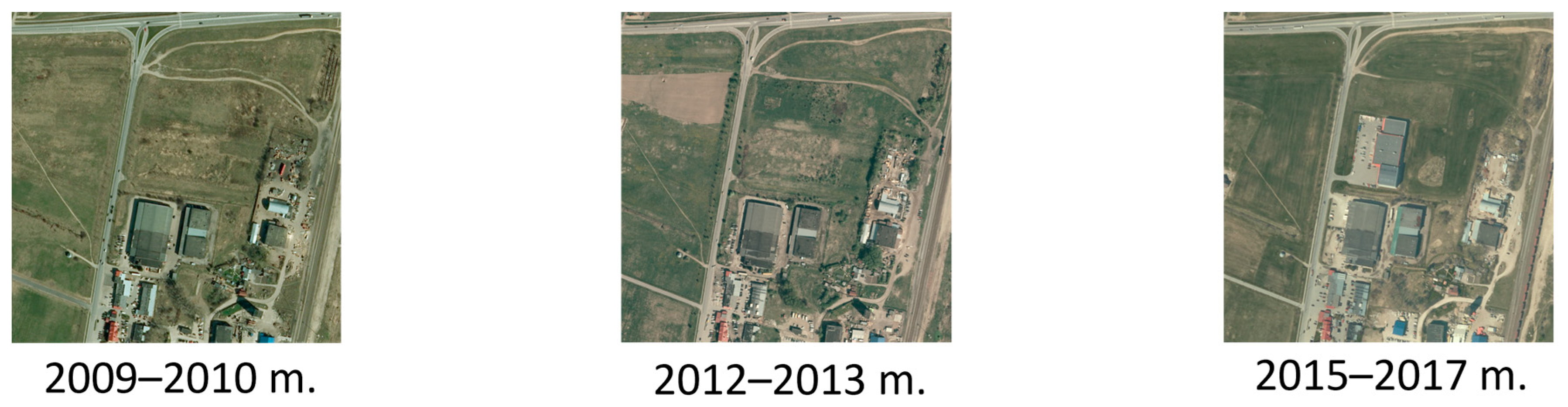
The changes in the land use (for example, new buildings, forests, agricultural land) can be identified from the series of aerial images of the same location. The example of such an idea is demonstrated in Figure 1 as the new buildings appear in the aerial image of the last period.
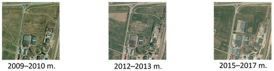
Figure 1.
Example of view difference at the same location in different periods.
Dynamics of indicators reflecting changes in buildings, forests, and other land use may determine a development rate of the region. By analyzing change speed of different municipalities, it is possible to identify clusters of similar development patterns. Visual data of Lithuania were selected for the analysis to track changes in the series of visual information and interpret the generalized results. The research focuses on two main objectives:
- To create a machine learning (ML) model, which enables the ability to obtain interpretable values on the local level for images of different periods and process the results at a detailed level;
- To demonstrate the applicability of the transfer learning approach in the ML model training process.
Different data sources for visual data were investigated. The requirements for the data were to ensure the adequate resolution of the images and to provide historical data. For example, Copernicus Sentinel Missions [21] do not fit these criteria due to low resolution for the building segmentation and unavailable historical data. Admittedly, the accuracy of the model can be improved by enhancing image resolution. Shermeyer and Etten suggested a technique to apply super-resolution to satellite images and concluded that such approach yielded a 13–36% improvement of mean average precision as the best results when detecting objects [22]. The image resolution can also be enhanced by applying a discrete wavelet transform [23]. Furthermore, Sentinel-2 data were used to perform pixel-wise classification of the built-up areas [24,25]. However, the lack of historical data is a major issue in rejecting some data sources. A digital raster orthophoto map at scale 1:10,000 of the Republic of Lithuania (ORT10LT) covers three different periods (2009–2010, 2012–2013, 2015–2017) and has an acceptable quality of images. The ORT10LT is provided by the State Enterprise National Centre for Remote Sensing and Geoinformatics “GIS-Centras” (SE “GIS-Centras”). Thus, this dataset was chosen for the analysis.
One of the issues that must be considered in the analysis of a time series of remote sensing data is stability of the model accuracy for images of different periods. For instance, if model accuracy for the images of one period is 90%, and another of 86%, it would be unclear whether the error appears due to labeling that does not match the actual information in the image of the specific period or due to the error of the machine learning (ML) model. Thus, it is important to ensure that accuracy for images of different periods is consistent. The ORT10LT images of different periods have different quality due to the image spectrum and resolution. The resolution of ORT10LT images in the first period was 0.5 m × 0.5 m and 8 bit RGB depth (7 bit effective); for the images of the second and third periods, the resolution increased to 0.25 m × 0.25 m per pixel. The color depth for the images in the second period was 8 bit RGB and 16 bit for the images of the third period. The changes in spectrum and resolution parameters were caused by the fact that in time, technical capabilities enabled attaining better quality. The technology jump can be demonstrated by the fact that before 2000, visual data for the same region were available only in grey scale compared to the current RGB of 16 bit depth.
4.2. Methodology Overview
A scheme for the suggested ML model training is provided in Figure 2. The training process consists of three main steps and is based on the concept of the transfer learning. The DeepLabv3 model (M) with a ResNet50 backbone is initialized with random parameters. In the first step, the model pretrained on the ImageNet data is loaded (M1). The second and third steps are dedicated to adjusting the model for the specific problem and contains training the model on coarse (M12) and fine-tuning (M123) datasets. The coarse dataset was generated automatically by selecting different locations and labeling the images based on the Open Street Map (OSM) data. However, the ground truth data may vary due to the time delay between the actual changes, which are visible in images and data input to registers or external databases. This is a reason why an additional step with training on the fine-tuning dataset was added. The fine-tuning dataset was created according to the same principles as the coarse dataset, but the images were manually reviewed and only the ones for which labeled data meet the visual information were used in the training process. Both coarse and fine-tuning datasets cover all three analyzed periods. As the images of different periods have different quality, they were normalized to match the lowest quality (oldest in time).
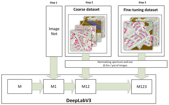
Figure 2.
Scheme of ML model training steps.
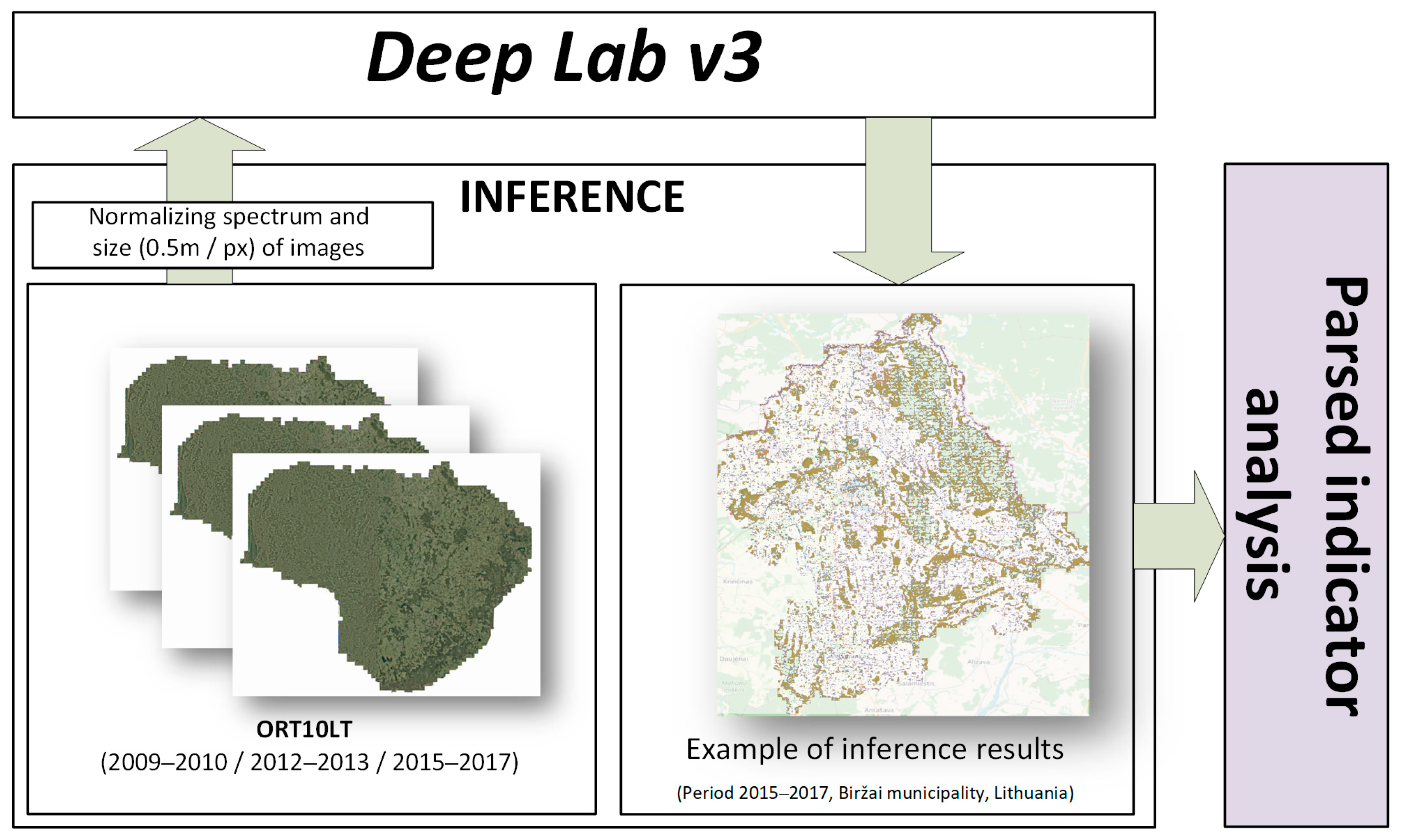
The scheme of ML model application is provided in Figure 3. The analyzed images are normalized according to parameters used in the training step. The preprocessed images are fed into the ML model and return the inference results. The interpretation of the obtained results depends on the analysis level.
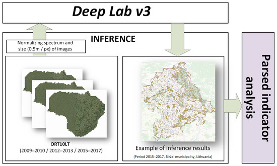
Figure 3.
Scheme of ML model application.
4.3. Dataset Collection and Preprocessing
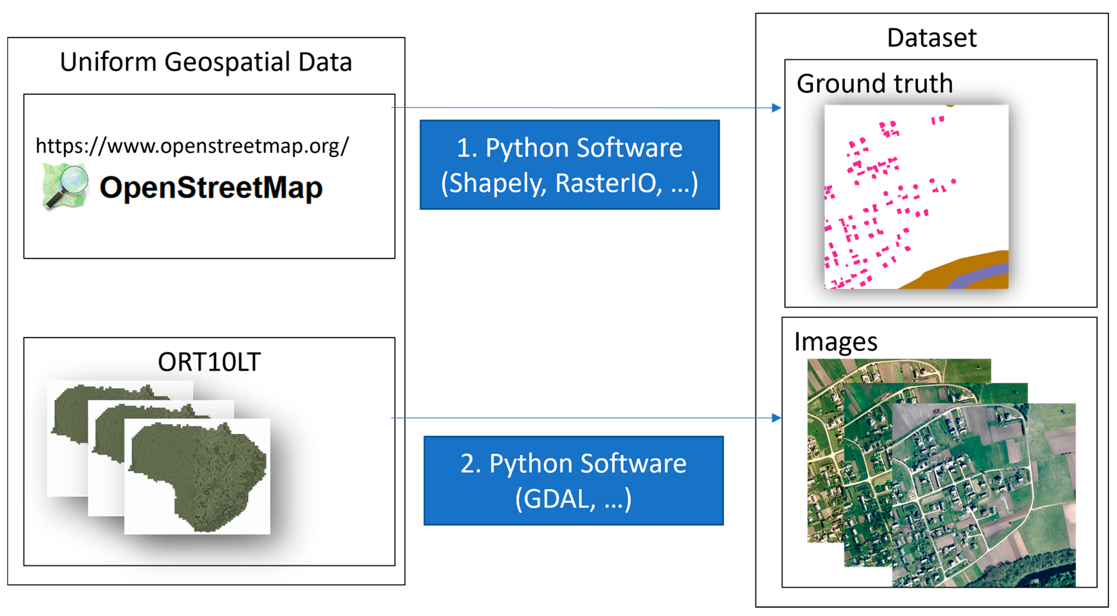
The ORT10LT is the digital orthophoto graphic map M 1:10,000 of the territory of the Republic of Lithuania. It is based on aerial photographs and is created in periods of 3 years. Images of periods of 2009–2010, 2012–2013, 2015–2017 were selected as a source of country-specific visual information. The OSM data were used for labeling as ground truth source. The labeling process consists of two steps. The first step is dedicated to collecting vector data from OSM data. In the second step, the GDAL library is employed to rasterize OSM vectors on geographical images. The labeling process is defined in Figure 4.
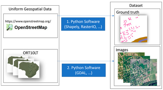
Figure 4.
The scheme of two-step data labeling process.
The OSM data can be used to define labels of fine level categories based on the purpose of land use type, for example, commercial, residential, educational, agricultural, and industrial. For this research, 4 generalized classes were selected to represent houses, forests, water, and other categories. The labels of the selected categories were defined as polygons (vector data from database). The software for labeling was written by the authors in the Python programming language. It uses models from the GluonCV toolkit with deep learning framework MXNet and geographic data processing library GDAL (for transformations from coordinates to pixels and from vector to raster coordinates). All data are represented as images (or can be viewed as 3 × 1024 × 1024 tensors). The ground truth labels are represented as indexed images of the respective height and width. After the inference is performed, the indexed images are associated to metadata of geographical position (ESRI world file was used in the research). For the complete overview of results, the images were combined into a mosaic.
Finally, following the dataset analysis, two types of problems were identified in the selected dataset:
- Logical—the OSM data do not always match the objects in images due to ill-timed mapping or changes in the environment as time passes. For example, a building is identified in the image but the label in OSM data is absent or new houses have been built recently and are not detected in the images of older periods.
- Quality—the results for images taken in different periods or locations may vary due to lighting and resulting shadows (early morning vs. afternoon); different angles at which the images were taken; different equipment used to take the images which results in different color response and dynamic range (some images are blurry because the photos were taken in early morning or at night).
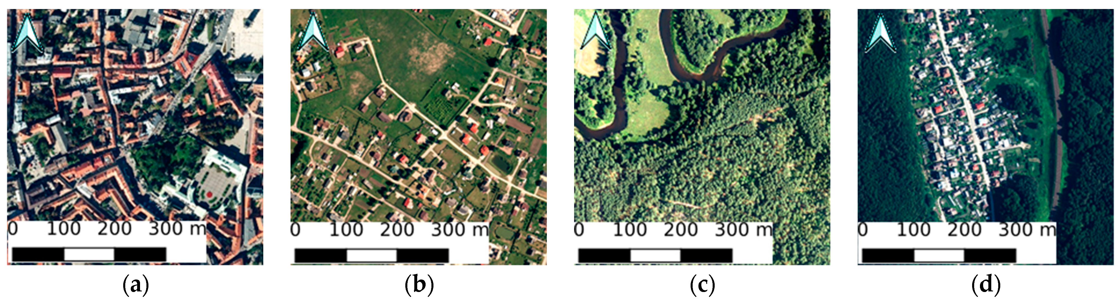
In order to ensure that training data represent the complete variety of analyzed classes, the images were prepared by combining two image selection approaches. For the first part of the dataset, a random building from the OSM database was selected and centered in the image of 1024 × 1024 pixels. This part guarantees that there is a significant part of labeled buildings in the dataset either from urban or rural areas. For the second part of the dataset, images were constructed by the same technique but selecting random points of the country as the image center. The majority of the Lithuanian landscape is identified as forests or fields. Therefore, this class mostly generates images which represent vegetation class. Finally, for the coarse training dataset, 5000 locations were selected (4000 with buildings and 1000 with vegetation, covering a total area of 1250 km2), resulting in 15,000 images (5000 images for each period, 3 images of the same location). Coarse validation set was created based on the same principles for 1000 locations (3000 images). The combination of image selection techniques and a relatively large number of images enables reducing the impact of the logical problem. Examples of different locations are provided in Figure 5.

Figure 5.
Sample images selected with a house centered (a,b) and random (c,d) which represent a diverse land use types, such as city (a), outskirts (b), vegetation (c), and village (d).
The fine-tuning dataset was created according to the same principles; however, the images were manually reviewed by removing the ones for which the labeled data did not meet the actual visible data. Such preparation of a dataset is a time-consuming process and requires thoroughness. Thus, the prepared dataset is small compared to the one prepared automatically. Ultimately, 321 locations (210 with buildings and 111 with vegetation, covering a total area of 80 km2) were selected. Fine-tuning validation set consists of 32 locations (96 images).
To solve the problems related to the different quality of images, normalization procedure was used as follows:
- Resolution was normalized to 0.5 m/pixel to fit the resolution of the lowest quality images;
- Contrast was normalized using a 2–98% percentile interval; all pixels over and under the interval were clipped to minimum or maximum values;
- Standard computer vision normalization procedure was applied to transform images so that the dataset distribution mean value is equal to 0 and standard deviation value is equal to 1 for each channel. The normalization procedure was performed with the assumption that initial distribution has mean values equal to 0.485, 0.456, and 0.406 and standard deviation values equal to 0.229, 0.224, and 0.225 for red, green, and blue channels, respectively. The values applied to normalize tensors are based on the statistical analysis of over 1.2 million images of ImageNet dataset.
4.4. Training Computer Vision Model
Various deep neural network architectures can be employed to detect changes in the satellite images. The network that combines DilatedResNet50 backbone, atrous convolutions, and spatial attention module was suggested to detect changes in high-resolution satellite images [26]. A network architecture with a Siamese-based backbone was suggested for remote sensing image change detection tasks [27]. The transfer learning approach was applied in [14] to train the U-Net model and obtain the change mask on the difference image.
The network configuration DeepLabv3 with a Resnet-50 backbone was chosen for computational model in this research. This architecture makes it possible to perform training with GluonCV MXNet framework on images of 1024 × 1024 pixels (3 × 1024 × 1024 tensor) using consumer GPU such as 2080 Ti with 11 GB RAM using minimum batch size. Although there are models which have better accuracy, GPU memory required to train such models is much higher [28]. For example, GluonCV MXNet model DeepLabv3+ with an Xception-71 backbone has approximately two percent better accuracy on the PASCAL VOC test compared to DeepLabv3 with ResNet-101. However, experimental results with 0.11.0 GluonCV and MXNet 1.8.0 versions for selected size images show that DeepLabv3 based on backbones Resnet50, Resnet101, and Resnet152 require approximately 10.5 GB, 14 GB, and 17 GB memory, in comparison to all DeepLabv3+ models with the same backbones which require 27 GB GPU memory measuring at the first epoch when memory usage is stabilized after training several batches. Thus, the selected model can be trained on the dataset generated from the whole country in a reasonable computational time and provide results of practically acceptable accuracy. The training was carried out on Cluster 3× servers with 2×AMD EPYC 7452 32-Core Processor and NVIDIA A100-PCIE-40GB with 512 GB RAM with batch size 4. As mentioned previously, automatically generated labels do not always match the actual class in images due to changes in the environment or mislabeled areas. Moreover, there are detection regions which represent a single class (for example, forest only). Focal loss focuses on misclassified examples and shows good practical results in dealing with imbalanced data. Thus, it was used as a loss function instead of Softmax entropy loss [25]. Focal loss is defined by the following equation [29]:
where α is for α-balanced form to reduce impact for detection outliners; γ is the focal factor. If γ = 0, focal loss corresponds to cross-entropy loss. If higher γ values are applied, the impact of easy examples is reduced, and the total loss value is scaled down. This leads to higher probability of correcting misclassified examples. The class classification function has the following definition:
where y specifies the ground truth class y ∈ {±1} and p ∈ [0,1] is the model probability for the class. For this experiment, α = 0.25 and γ =2.
The technical specifications of the selected model are as follows:
- Input layer: 1024 × 1024 pixels (result taken from 896 × 896 pixels) ~448 m × 448 m (or ~0.2 km2) area;
- Coarse learning: learning rate 5 × 10⁻⁴; momentum 0.5; 5000 samples per epoch;
- Fine-tune learning: learning rate 5 × 10⁻⁵; momentum 0.1; 100 samples per epoch.
The model trained under the suggested approach is further referred to as M123, meaning that it includes all three steps (pretrained weights on ImageNet, coarse learning, and fine-tuned learning) of the transfer learning process. In order to demonstrate the importance of each step and the advantage of the transfer learning, in total six DeepLabv3 models with a ResNet50 backbone were trained using combinations of the steps provided in Figure 2. The strategies are summarized in Table 1.

Table 1.
Summarized strategies used in training models.
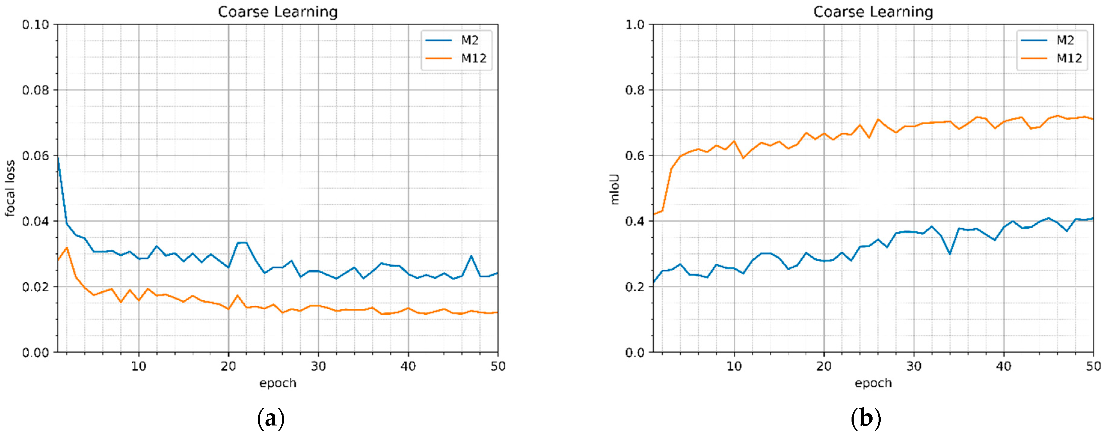
The mean value of the focal loss (1) and mIoU (mean intersection over union) values for the coarse validation set during 50 training epochs on the coarse dataset of the models M2 and M12 are provided in Figure 6a,b, respectively. Figure 6 shows that using the pretrained on the ImageNet model (M12) gives significantly better results (smaller focal loss value and larger mIoU value) from the beginning of the training.
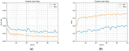
Figure 6.
Evaluation metrics (focal loss (a) and mIoU (b)) for coarse validation set during the coarse training of the models M2 (without pretraining on ImageNet) and M12 (with pretraining on ImageNet).
During the training process, the validation set is used to evaluate the accuracy of the model for the unseen data. The values of the focal loss, mIoU, and pixel accuracy for the coarse validation set after the training of the models M2 and M12 are provided in Table 2. Using a pretrained on ImageNet model results in approximately 1.7 times higher mIoU value and the focal loss value lower than 0.05.
Table 2.
Focal loss, mIoU, and pixel accuracy values for the coarse validation set after the training.
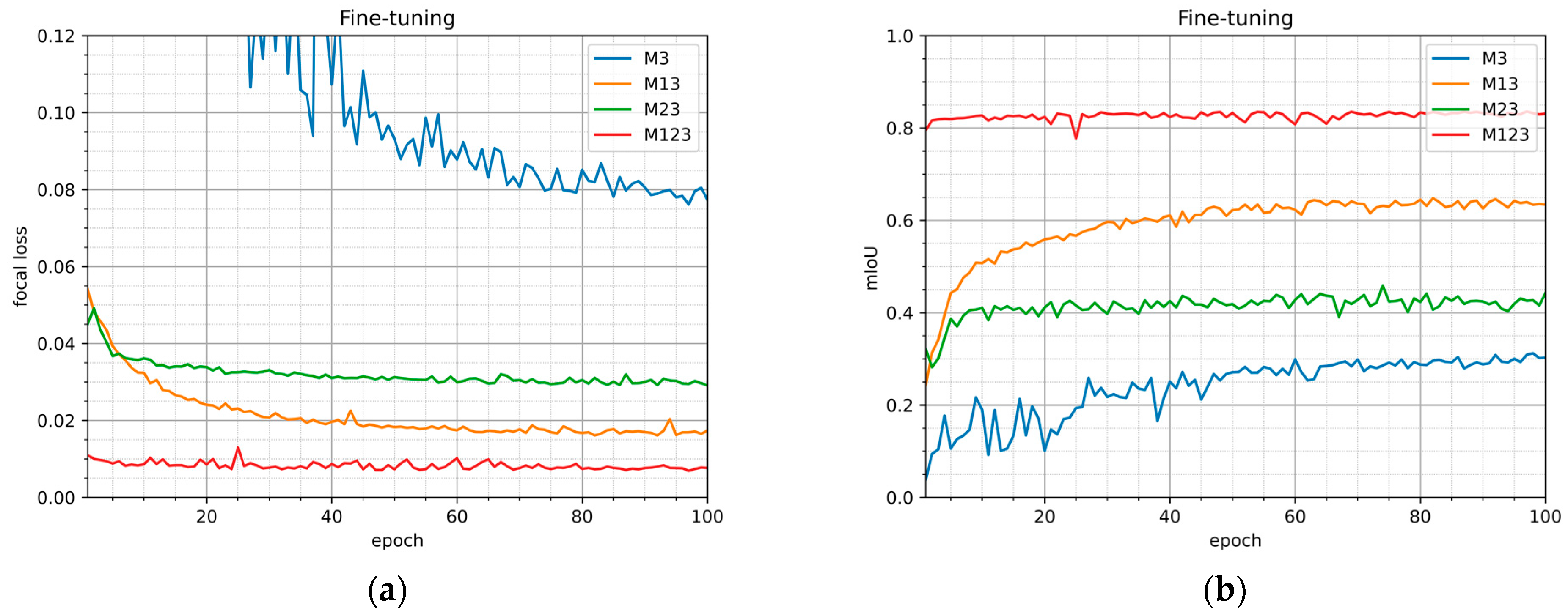
Similarly, the analysis during the training on the fine-tuning dataset for the models M3, M23, M13, and M123 was performed. The mean value of the focal loss (1) and mIoU (mean intersection of the union) values for the fine-tuning validation set during 100 training epochs of the models M3, M23, M13, and M123 are provided in Figure 7a,b, respectively. The largest loss and smallest mIoU values were obtained for the M3 model. This model also shows the largest progress in learning (biggest difference between the values in the starting and finishing epochs), as the model is trained with initial random coefficients and starts to extract useful features and patterns. For the first 5 epochs, models M13 and M23 show similar loss and mIoU values. In later epochs, values obtained for M23 converge in first 10 epochs, whereas values obtained for the M13 model demonstrate further learning. This phenomenon is caused by the fact that image sets of completely different nature were used in the different steps of training M13; that is, the ImageNet dataset was used for the pretraining, and the fine-tuning dataset was used in the adjustment step. The pretrained model can extract basic features, such as contours and patterns, but the learning proceeds to adjust for the fine-tuning dataset of aerial images. During training of the M23, the model is already trained on a similar dataset and does not show a significant improvement. The best loss and mIoU values were demonstrated by the M123 model. This model was created according to the suggested training process, and the training on the fine-tuning dataset was performed after training the pretrained model on the coarse dataset. However, there was just a slight improvement for this model. The pretrained models M23 and M123 start from loss function values close to the ones which the models M2 and M12 converged after training models on the coarse dataset (Figure 6). The accuracy estimates depend on the validation set. It should be noted that in the fine-tuning validation dataset some inconsistencies of labeling are clarified; therefore, it results in higher loss value.
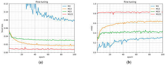
Figure 7.
Evaluation metrics (focal loss (a) and mIoU (b)) for fine-tuning validation set during the fine-tune training of the models M3, M23, M13, M123.
The values of the focal loss, mIoU, and pixel accuracy for the fine-tuning validation set after the training of the models M3, M13, M23, and M123 are provided in Table 3. It is demonstrated that using a pretrained on ImageNet model results in approximately 2 times higher mIoU value (M13 and M123 compared to M3 and M23 values, respectively). In addition, the highest mIoU and pixel accuracy values were obtained for the model that was created using all three steps of the suggested training scheme.
Table 3.
Focal loss, mIoU, and pixel accuracy values for the fine-tuning validation set after the training.
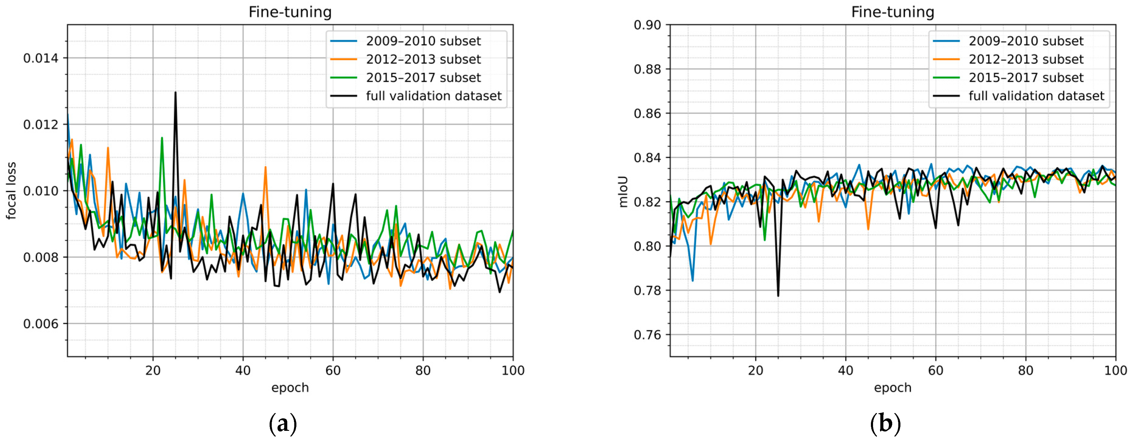
Images of all three periods were included in training and validation datasets. The suggested model training process had an image normalization step. This step was incorporated in the data preprocessing to maintain stable accuracy of the model and ensure that using images of different periods in application is valid. To demonstrate that using normalized images from different periods do not cause significantly different accuracy, loss and mIoU values for fine-tuning validation subsets grouped by period are provided in Figure 8a,b, respectively.
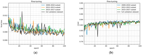
Figure 8.
Evaluation metrics (focal loss (a) and mIoU (b)) for fine-tuning validation set and its subsets during the fine-tune learning.
The focal loss, mIoU, and pixel accuracy values of the model M123 for the validation subsets of images from different periods after the training are provided in Table 4. The focal loss values are lower than 0.01 for all subsets and the dataset itself. The mIoU and pixel accuracy values of the subsets differ less than 2% with respect to the mIoU and pixel accuracy value of the full dataset.
Table 4.
Focal loss, mIoU, and pixel accuracy values for the fine-tune validation subsets of different periods for the M123 model after the training.
The normalized confusion matrices of model M123 segmentation results for the fine-tune validation set and its subsets of different periods are given in Figure 9. The confusion matrices include all classes used in segmentation, that is, house, forest, water, and other. The matrices show that over 90% of predictions match the true labels for forest, water, and other classes for full validation set and its subsets. In addition, the predictions for the house class exceeded 75% of the true house class labels in the dataset and its subsets. It should be noted that the most frequent false prediction for house class was as other class. The reason for this phenomenon is that ground truth components of houses have sharp edges and complex geometry, and these features are not maintained in the inference results. Moreover, the components are small, and the number of house components is large compared to other classes.
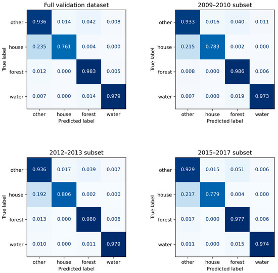
Figure 9.
Normalized confusion matrix of M123 segmentation results for full fine-tuning validation set and its subsets of different periods.
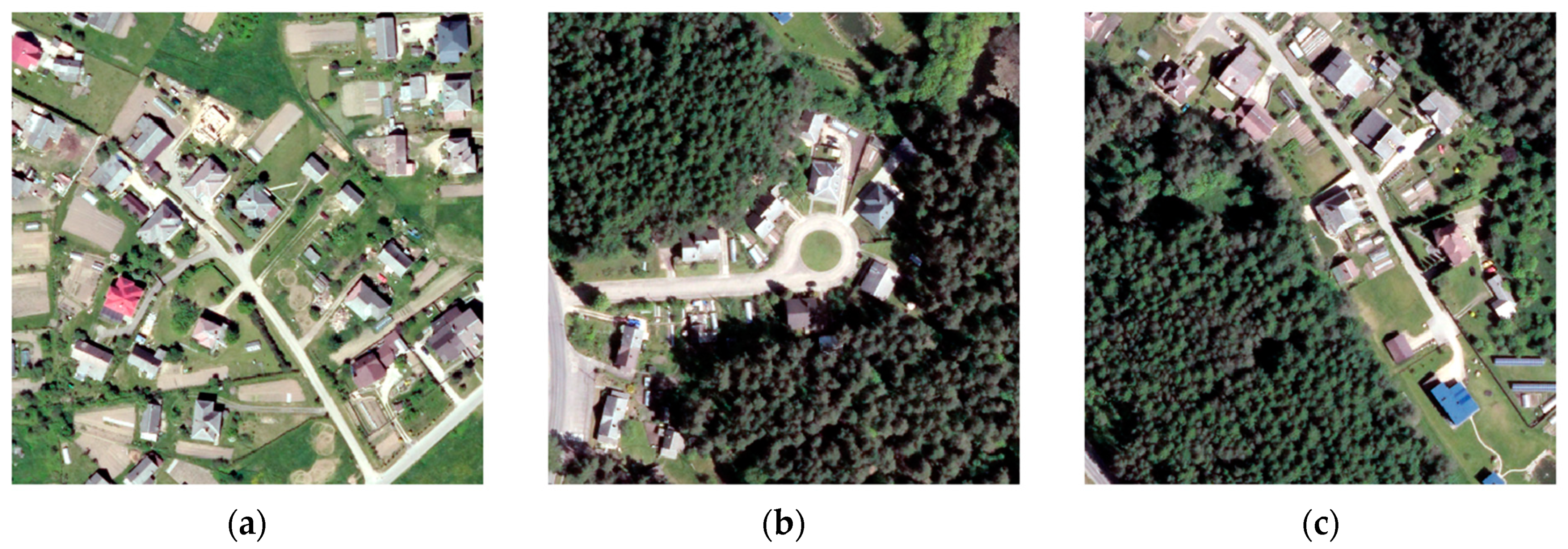
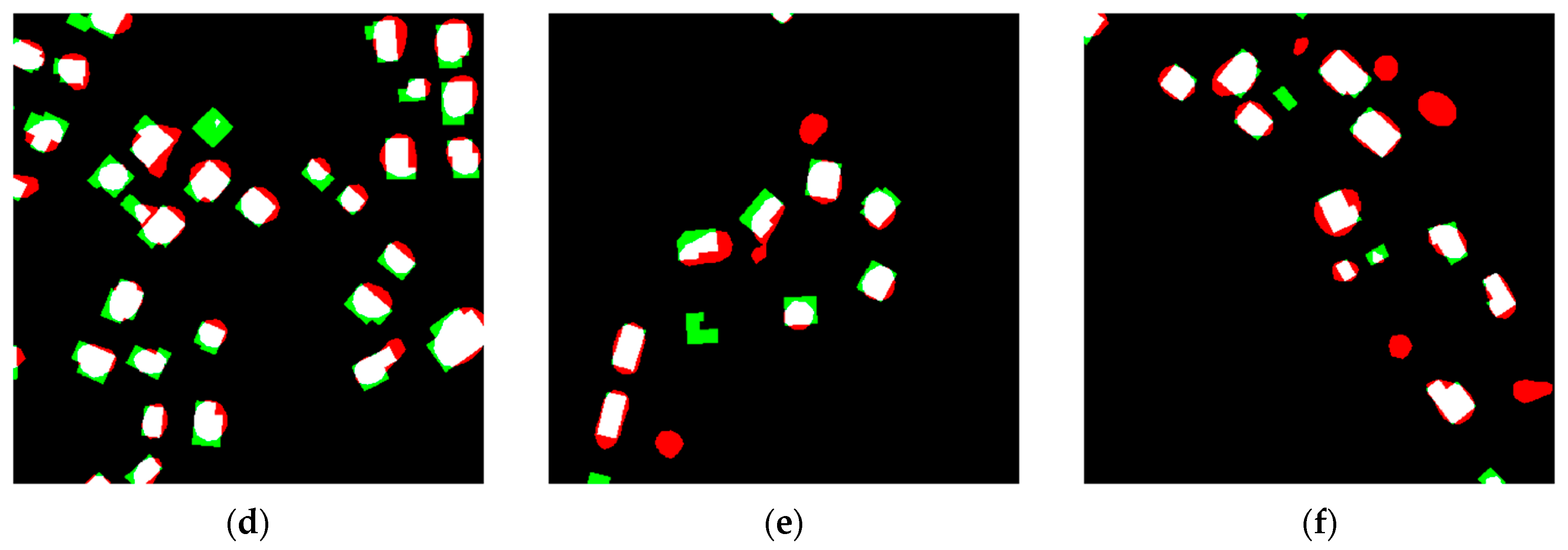
The examples of images and their inference results compared to ground truth are provided in Figure 10. White color represents intersection of ground truth and inference results, green color represents ground truth, which is not covered by the inference results, and red color represents inference results which do not cover ground truth. The main dataset problems are demonstrated in the examples given in Figure 10. Firstly, the house under construction is included in ground truth but was not detected by the model (Figure 10a,d). Secondly, the house is not detected due to shadowing (Figure 10b,e). Finally, there are buildings that are detected by the model but were not included in the ground truth (Figure 10b,c,e,f). The examples demonstrate that the inference results correspond to ground truth. The calculations show that more than 80% of house components in the ground truth have more than 50% overlap with the inference results.


Figure 10.
Examples of the original images (a–c) and results of their inference results compared to the ground truth (d–f). White color represents the match between ground truth and inference, green represents the ground truth which is not covered by the inference results, and red represents the inference results which do not cover ground truth.
5. Results
The model was developed to detect four main classes (houses, forest, water, and other). The direct results obtained with the developed model enables the ability to analyze and interpret the results on different levels.
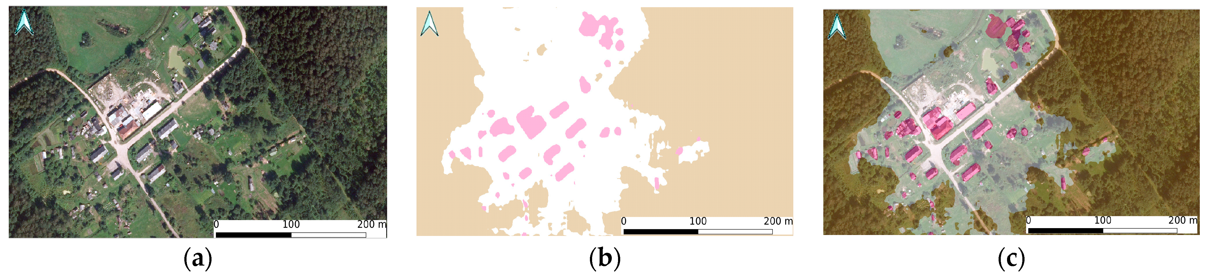
On the finest level, the results of the model can be analyzed locally and visualized using standard map software, i.e., QGis and ArcGis. Figure 11 and Figure 12 demonstrate the results obtained with the model using the QGIS software. The results show the identified buildings, water, and forest areas.
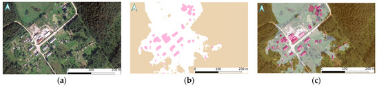
Figure 11.
The example of inference using image from 2009–2010 dataset with a random position: (a) original ORTO10 view; (b) inference results; (c) overlay of original image and transparent inference results.
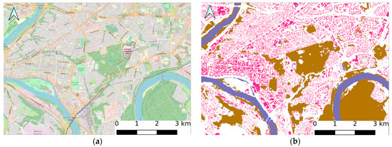
Figure 12.
The segmentation results on the finest level: (a) OSM map view of Kaunas city center; (b) processed data of Kaunas city center of the selected time period (2009–2010) with segmented buildings (magenta), water (blue), forest/trees (brown), and other (white) categories.
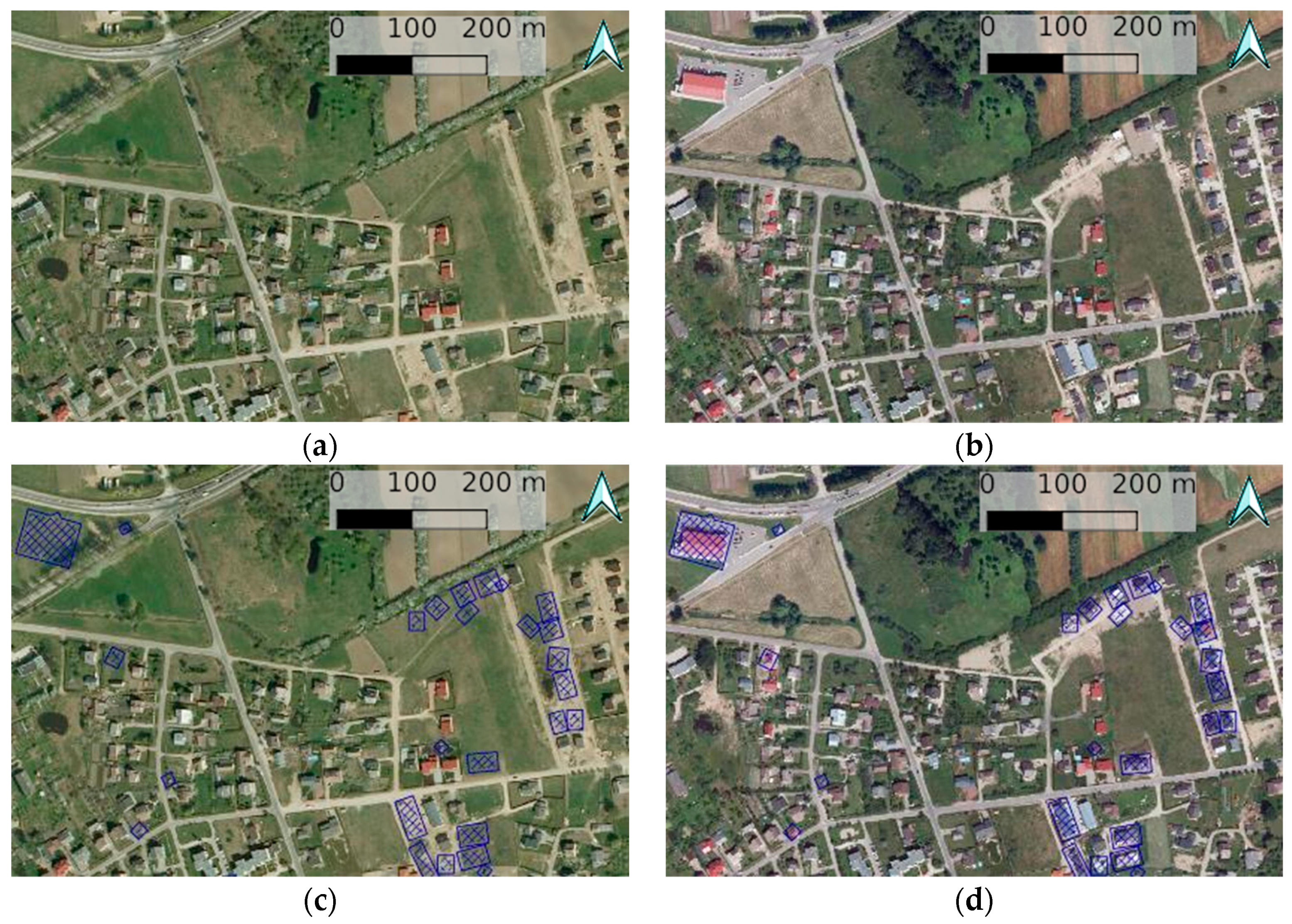
The obtained results of different periods can be applied to highlight changes between the images of two periods in the same location. The initial images of periods 2009–2010 and 2012–2013 and the modified ones with a layer which represents change in building class are provided in Figure 13.
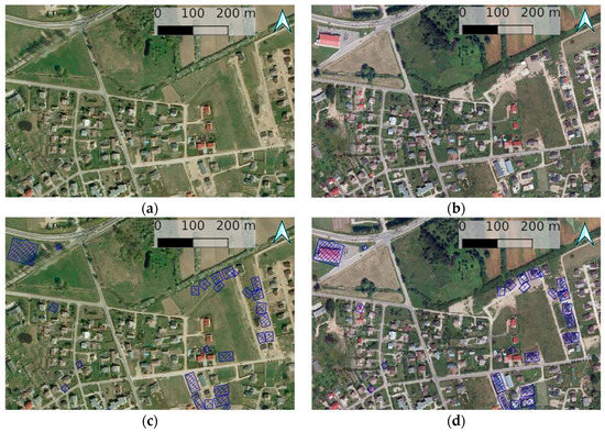
Figure 13.
The example of change identification: (a,b) Original ORTO10LT images of periods 2009–2010 and 2012–2013, respectively; (c,d) images with a hatch layer which represents mismatch of the building class in segmentation results.
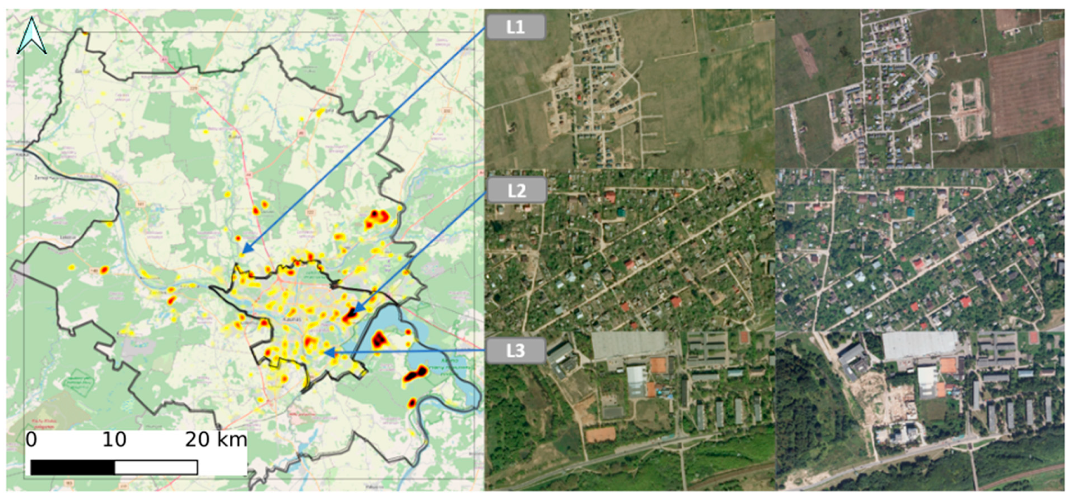
On the middle level, the model can be applied to identify the urban change of the region by creating a heat map. The country was divided into a grid and the value of a grid cell was determined by the total number of buildings detected per grid cell. Then, the difference between the respective grid cells of different periods was calculated and visualized in Figure 14 together with example images of three different locations L1, L2, and L3 for both periods. Location L1 represents the area of urban expansion as a new block of houses is expanding in the suburbs. Location L2 represents an existing block of allotment gardens which in time becomes a residential area as small old summer houses are replaced by new detached houses. Location L3 was chosen to demonstrate development of a new block of apartment buildings.

Figure 14.
Heat map of difference between total number of buildings in grid cell for periods 2009–2010 and 2012–2013 in Kaunas city and region and examples of images in locations L1, L2, L3.
The same methodological approach can be applied to remote sensing data of higher frequency, for example, satellite images. Using more data points would enable performing an analysis of urban change dynamics at a more detailed level and forecast future growth patterns of the monitored region.
Obviously, more generalized data can be useful in urban development analysis at the municipality level to plan infrastructure, identify patterns, and make political decisions.
6. Conclusions
Semantic segmentation of satellite or aerial images is usually applied to small regions and specific problems, such as building extraction [30,31,32,33,34]. Research on a higher level (city or country) of satellite images is mainly focused on estimating socio-economic indicators or poverty level [18,35,36]; thus, they were usually focused on the final result rather than the process itself. This publication fills in the missing gaps by providing a methodological approach on how to prepare the training data for coarse and fine-tune learning, that is, how to ensure a variety of different classes and deal with images of different quality. The provided methodological approach can be applied in different countries for aerial or satellite images in order to determine the urban change patterns. In this work, the transfer learning technique was applied for creating a machine learning model according to the training scheme which was initially proposed in [20]. The DeepLabv3 model with a ResNet50 backbone initially pretrained on the ImageNet data was selected. The following two steps of learning on coarse and fine-tuning datasets were carried out to adjust the model. In the coarse learning step, the model was trained on a dataset automatically labeled with OSM data. This enabled learning features specific to the aerial dataset. The fine-tuning step was dedicated to increasing the accuracy of the model, as the manually revised data were used in training. In this article we consider the importance of each step in the training scheme. To demonstrate the benefits of using the transfer learning approach, five additional machine learning models were strained under different strategies which included various combinations of training steps. The model, which was created with respect to the suggested procedure, demonstrated more accurate results compared to the other five models which were developed using various combinations of learning steps. Obviously, this model is trained on the largest variety of images (ImageNet, coarse, and fine-tuning datasets) and its training lasts the longest time if time of the initial training on ImageNet is considered. It was also demonstrated that images of different periods do not have bias, as the focal loss value is low for all subsets and mIoU and the pixel accuracy values have less than 2% difference compared to the respective values of the full dataset.
It was demonstrated that the neural network using OSM as a ground truth dataset is capable of making semantic segmentation with reasonable accuracy. However, expert input is necessary in the data preparation stage to consider the differences in mapping, such as the use of the most recent ground truth data with the assumption that there are not many changes in data over the years. Normalization of the different quality images on spectrum and contrast enables analyzing and interpreting results on various levels for the series of images from different periods. The generalized results could be used to detect urban change patterns by using a heat map of difference, while for the fine level analysis, it is possible to review local changes on a map of a specific location.
Analysis and estimation of urban growth patterns could be used for several purposes and different parties. For instance, investors might use the identification of the growth of the households to purchase real estate for rent purposes or for reselling real estate. The city usually grows with respect to housing prices. That is, if housing prices are high in one area of the city, consumers tend to purchase houses in parts of city where prices are lower. Later, the price growth usually shifts to balance supply and demand. Other users might be government, which should provide region plans based on the current situation and future estimates. Housing development and population density should be taken into consideration during planning infrastructure objects such as schools, hospitals, and the road network. Planning of such infrastructure in advance could lead to lower construction costs, more efficient regions, and, therefore, better sustainable management and higher productivity. Thus, the proposed methodological approach can be applied in developed markets to obtain more accurate real-time urban growth analysis and in developing markets to better understand the current market situation, especially if statistical data are limited.
Author Contributions
Conceptualization, Andrius Kriščiūnas and Valentas Gružauskas; methodology, Tautvydas Fyleris, Andrius Kriščiūnas, Valentas Gružauskas and Dalia Čalnerytė; software, Tautvydas Fyleris, Andrius Kriščiūnas and Valentas Gružauskas; validation, Valentas Gružauskas, Dalia Čalnerytė and Rimantas Barauskas; formal analysis, Valentas Gružauskas, Dalia Čalnerytė and Rimantas Barauskas; investigation, Tautvydas Fyleris and Dalia Čalnerytė; resources, Andrius Kriščiūnas and Rimantas Barauskas; data curation, Andrius Kriščiūnas and Valentas Gružauskas; writing—original draft preparation, Valentas Gružauskas and Dalia Čalnerytė; writing—review and editing, Tautvydas Fyleris, Andrius Kriščiūnas and Rimantas Barauskas; visualization, Tautvydas Fyleris; supervision, Andrius Kriščiūnas and Rimantas Barauskas; project administration, Andrius Kriščiūnas; funding acquisition, Andrius Kriščiūnas All authors have read and agreed to the published version of the manuscript.
Funding
This research was supported by the Research, Development, and Innovation Fund of Kaunas University of Technology (project grant No. PP91L/19).
Data Availability Statement
The OSM data are freely available from the Open Street Map website https://wiki.openstreetmap.org (accessed on 22 December 2021). The ORT10LT is available with limited access from https://www.geoportal.lt/ (accessed on 22 December 2021).
Conflicts of Interest
The authors declare no conflict of interest. The funders had no role in the design of the study; in the collection, analyses, or interpretation of data; in the writing of the manuscript, or in the decision to publish the results.
References
- Dadashpoor, H.; Azizi, P.; Moghadasi, M. Analyzing spatial patterns, driving forces and predicting future growth scenarios for supporting sustainable urban growth: Evidence from Tabriz metropolitan area, Iran. Sustain. Cities Soc. 2019, 47, 101502. [Google Scholar] [CrossRef]
- Liang, X.; Liu, X.; Li, D.; Zhao, H.; Chen, G. Urban growth simulation by incorporating planning policies into a CA-based future land-use simulation model. Int. J. Geogr. Inf. Sci. 2018, 32, 2294–2316. [Google Scholar] [CrossRef]
- Serasinghe Pathiranage, I.S.; Kantakumar, L.N.; Sundaramoorthy, S. Remote Sensing Data and SLEUTH Urban Growth Model: As Decision Support Tools for Urban Planning. Chin. Geogr. Sci. 2018, 28, 274–286. [Google Scholar] [CrossRef] [Green Version]
- Xie, M.; Jean, N.; Burke, M.; Lobell, D.; Ermon, S. Transfer learning from deep features for remote sensing and poverty mapping. In Proceedings of the 30th AAAI Conference on Artificial Intelligence, AAAI 2016, Phoenix, AZ, USA, 12–17 February 2016; pp. 3929–3935. [Google Scholar]
- Macků, K.; Voženílek, V.; Pászto, V. Linking the quality of life index and the typology of European administrative units. J. Int. Dev. 2022, 34, 145–174. [Google Scholar] [CrossRef]
- Gevaert, C.M.; Persello, C.; Sliuzas, R.; Vosselman, G. Monitoring household upgrading in unplanned settlements with unmanned aerial vehicles. Int. J. Appl. Earth Obs. Geoinf. 2020, 90, 102117. [Google Scholar] [CrossRef]
- Emilien, A.-V.; Thomas, C.; Thomas, H. UAV & satellite synergies for optical remote sensing applications: A literature review. Sci. Remote Sens. 2021, 3, 100019. [Google Scholar] [CrossRef]
- Shi, W.; Zhang, M.; Zhang, R.; Chen, S.; Zhan, Z. Change detection based on artificial intelligence: State-of-the-art and challenges. Remote Sens. 2020, 12, 1688. [Google Scholar] [CrossRef]
- Cui, B.; Zhang, Y.; Yan, L.; Wei, J.; Wu, H. An unsupervised SAR change detection method based on stochastic subspace ensemble learning. Remote Sens. 2019, 11, 1314. [Google Scholar] [CrossRef] [Green Version]
- Donaldson, D.; Storeygard, A. The view from above: Applications of satellite data in economics. J. Econ. Perspect. 2016, 30, 171–198. [Google Scholar] [CrossRef] [Green Version]
- Celik, T. Unsupervised change detection in satellite images using principal component analysis and κ-means clustering. IEEE Geosci. Remote Sens. Lett. 2009, 6, 772–776. [Google Scholar] [CrossRef]
- de Jong, K.L.; Sergeevna Bosman, A. Unsupervised Change Detection in Satellite Images Using Convolutional Neural Networks. In Proceedings of the 2019 International Joint Conference on Neural Networks (IJCNN), Budapest, Hungary, 14–19 July 2019; pp. 1–8. [Google Scholar] [CrossRef] [Green Version]
- Xue, D.; Lei, T.; Jia, X.; Wang, X.; Chen, T.; Nandi, A.K. Unsupervised Change Detection Using Multiscale and Multiresolution Gaussian-Mixture-Model Guided by Saliency Enhancement. IEEE J. Sel. Top. Appl. Earth Obs. Remote Sens. 2021, 14, 1796–1809. [Google Scholar] [CrossRef]
- Liu, J.; Chen, K.; Xu, G.; Sun, X.; Yan, M.; Diao, W.; Han, H. Convolutional Neural Network-Based Transfer Learning for Optical Aerial Images Change Detection. IEEE Geosci. Remote Sens. Lett. 2020, 17, 127–131. [Google Scholar] [CrossRef]
- Zhang, Y.; Fu, L.; Li, Y.; Zhang, Y. Hdfnet: Hierarchical dynamic fusion network for change detection in optical aerial images. Remote Sens. 2021, 13, 1440. [Google Scholar] [CrossRef]
- Jiang, H.; Hu, X.; Li, K.; Zhang, J.; Gong, J.; Zhang, M. PGA-SiamNet: Pyramid feature-based attention-guided siamese network for remote sensing orthoimagery building change detection. Remote Sens. 2020, 12, 484. [Google Scholar] [CrossRef] [Green Version]
- Wurm, M.; Stark, T.; Zhu, X.X.; Weigand, M.; Taubenböck, H. Semantic segmentation of slums in satellite images using transfer learning on fully convolutional neural networks. ISPRS J. Photogramm. Remote Sens. 2019, 150, 59–69. [Google Scholar] [CrossRef]
- Jean, N.; Burke, M.; Xie, M.; Davis, W.M.; Lobell, D.B.; Ermon, S. Combining satellite imagery and machine learning to predict poverty. Science 2016, 353, 790–794. [Google Scholar] [CrossRef] [Green Version]
- Suraj, P.K.; Gupta, A.; Sharma, M.; Paul, S.B.; Banerjee, S. On monitoring development indicators using high resolution satellite images. arXiv 2018, arXiv:1712.02282. [Google Scholar]
- Fyleris, T.; Kriščiūnas, A.; Gružauskas, V.; Čalnerytė, D. Deep Learning Application for Urban Change Detection from Aerial Images. In GISTAM 2021: Proceedings of the 7th International Conference on Geographical Information Systems Theory, Applications and Management, Online, 23–25 April 2021; SciTePress: Setúbal, Portugal, 2021; pp. 15–24. [Google Scholar] [CrossRef]
- The Sentinel Missions. Available online: https://www.esa.int/Applications/Observing_the_Earth/Copernicus/The_Sentinel_missions (accessed on 9 February 2022).
- Shermeyer, J.; Van Etten, A. The Effects of Super-Resolution on Object Detection Performance in Satellite Imagery. In Proceedings of the IEEE/CVF Conference on Computer Vision and Pattern Recognition Workshops, Long Beach, CA, USA, 16–17 June 2019. [Google Scholar]
- Witwit, W.; Zhao, Y.; Jenkins, K.; Zhao, Y. Satellite image resolution enhancement using discrete wavelet transform and new edge-directed interpolation. J. Electron. Imaging 2017, 26, 023014. [Google Scholar] [CrossRef]
- Krupinski, M.; Lewiński, S.; Malinowski, R. One class SVM for building detection on Sentinel-2 images. In Photonics Applications in Astronomy, Communications, Industry, and High-Energy Physics Experiments 2019; International Society for Optics and Photonics: Wilga, Poland, 2019; Volume 1117635, p. 6. [Google Scholar]
- Corbane, C.; Syrris, V.; Sabo, F.; Pesaresi, M.; Soille, P.; Kemper, T. Convolutional Neural Networks for Global Human Settlements Mapping from Sentinel-2 Satellite Imagery. arXiv 2020, arXiv:2006.03267. [Google Scholar] [CrossRef]
- Song, K.; Jiang, J. AGCDetNet:An Attention-Guided Network for Building Change Detection in High-Resolution Remote Sensing Images. IEEE J. Sel. Top. Appl. Earth Obs. Remote Sens. 2021, 14, 4816–4831. [Google Scholar] [CrossRef]
- Ke, Q.; Zhang, P. CS-HSNet: A Cross-Siamese Change Detection Network Based on Hierarchical-Split Attention. IEEE J. Sel. Top. Appl. Earth Obs. Remote Sens. 2021, 14, 9987–10002. [Google Scholar] [CrossRef]
- Minaee, S.; Boykov, Y.Y.; Porikli, F.; Plaza, A.J.; Kehtarnavaz, N.; Terzopoulos, D. Image Segmentation Using Deep Learning: A Survey. IEEE Trans. Pattern Anal. Mach. Intell. 2021, 8828, 1–20. [Google Scholar] [CrossRef] [PubMed]
- Lin, T.-Y.; Goyal, P.; Girshick, R.; He, K.; Dollar, P. Focal Loss for Dense Object Detection (RetinaNet). In Proceedings of the IEEE International Conference on Computer Vision, Venice, Italy, 22–29 October 2017; pp. 2980–2988. [Google Scholar]
- Liu, Y.; Han, Z.; Chen, C.; DIng, L.; Liu, Y. Eagle-Eyed Multitask CNNs for Aerial Image Retrieval and Scene Classification. IEEE Trans. Geosci. Remote Sens. 2020, 58, 6699–6721. [Google Scholar] [CrossRef]
- Ye, Z.; Fu, Y.; Gan, M.; Deng, J.; Comber, A.; Wang, K. Building extraction from very high resolution aerial imagery using joint attention deep neural network. Remote Sens. 2019, 11, 2970. [Google Scholar] [CrossRef] [Green Version]
- Wu, G.; Shao, X.; Guo, Z.; Chen, Q.; Yuan, W.; Shi, X.; Xu, Y.; Shibasaki, R. Automatic building segmentation of aerial imagery usingmulti-constraint fully convolutional networks. Remote Sens. 2018, 10, 407. [Google Scholar] [CrossRef] [Green Version]
- Dornaika, F.; Moujahid, A.; El Merabet, Y.; Ruichek, Y. Building detection from orthophotos using a machine learning approach: An empirical study on image segmentation and descriptors. Expert Syst. Appl. 2016, 58, 130–142. [Google Scholar] [CrossRef]
- Vakalopoulou, M.; Karantzalos, K.; Komodakis, N.; Paragios, N. Building detection in very high resolution multispectral data with deep learning features. In Proceedings of the 2015 IEEE International Geoscience and Remote Sensing Symposium (IGARSS), Milan, Italy, 26–31 July 2015; pp. 1873–1876. [Google Scholar] [CrossRef] [Green Version]
- Al-Ruzouq, R.; Hamad, K.; Shanableh, A.; Khalil, M. Infrastructure growth assessment of urban areas based on multi-temporal satellite images and linear features. Ann. GIS 2017, 23, 183–201. [Google Scholar] [CrossRef]
- Albert, A.; Kaur, J.; Gonzalez, M.C. Using convolutional networks and satellite imagery to identify patterns in urban environments at a large scale. In Proceedings of the 23rd ACM SIGKDD International Conference on Knowledge Discovery and Data Mining, Halifax, NS, Canada, 13–17 August 2017; Part F1296. pp. 1357–1366. [Google Scholar] [CrossRef] [Green Version]


Publisher’s Note: MDPI stays neutral with regard to jurisdictional claims in published maps and institutional affiliations. |
© 2022 by the authors. Licensee MDPI, Basel, Switzerland. This article is an open access article distributed under the terms and conditions of the Creative Commons Attribution (CC BY) license (https://creativecommons.org/licenses/by/4.0/).