Cluster Nested Loop k-Farthest Neighbor Join Algorithm for Spatial Networks

Abstract

This paper considers k-farthest neighbor (kFN) join queries in spatial networks where the distance between two points is the length of the shortest path connecting them. Given a positive integer k, a set of query points Q, and a set of data points P, the kFN join query retrieves the k data points farthest from each query point in Q. There are many real-life applications using kFN join queries, including artificial intelligence, computational geometry, information retrieval, and pattern recognition. However, the solutions based on the Euclidean distance or nearest neighbor search are not suitable for our purpose due to the difference in the problem definition. Therefore, this paper proposes a cluster nested loop join (CNLJ) algorithm, which clusters query points (data points) into query clusters (data clusters) and reduces the number of kFN queries required to perform the kFN join. An empirical study was performed using real-life roadmaps to confirm the superiority and scalability of the CNLJ algorithm compared to the conventional solutions in various conditions.

1. Introduction

In this study, we investigate the efficient processing of k-farthest neighbor (kFN) join queries in spatial networks where the distance between two points is defined by the length of the shortest path connecting them. The kFN join combines each query point q in Q with the k data points in P that are farthest from the query point q, given a positive integer k, a set of query points Q, and a set of data points P. The kFN join query has real-life applications in recommender systems, where farthest neighbors can increase the variety of recommendations [1,2]. Farthest neighbor search is also an element in clustering applications [3], complete linkage clustering [4], and nonlinear dimensionality reduction algorithms [5]. Thus, being able to quickly process kFN join queries is an important practical concern for many applications [6,7,8,9,10,11,12,13,14].

Figure 1 shows an example of the kFN join between a set Q of query points and a set P of data points in a spatial network, where it is assumed that $k=1$, $Q=\{q_1,q_2,q_3\}$, and $P=\{p_1,p_2,p_3,p_4\}$ are given. In this paper, the kFN join is denoted as $Q{⋉}_{kFN}P$. In this example, the data points farthest away from $q_1$, $q_2$, and $q_3$ are $p_2$, $p_2$, and $p_3$, respectively, which can be represented by $Q{⋉}_{kFN}P=\{〈q_1,p_2〉,〈q_2,p_2〉,〈q_3,p_3〉\}$. Conversely, the query points farthest from $p_1$, $p_2$, $p_3$, and $p_4$ are $q_1$, $q_1$, $q_3$, and $q_1$, respectively, which can be represented by $P{⋉}_{kFN}Q=\{〈p_1,q_1〉,〈p_2,q_1〉,〈p_3,q_3〉,〈p_4,q_1〉\}$. This simply proves that kFN joins are not commutative, i.e., $Q{⋉}_{kFN}P\ne P{⋉}_{kFN}Q$. Note that this study considers $Q{⋉}_{kFN}P$. The facility location problem, which determines the competitive location of a new facility, such as garbage incinerators, crematoriums, chemical plants, supermarkets, and police stations, is very important in real life when using the kFN join query applications. Particularly, determining the optimal facility location is still an open problem [15,16]. Facing such a research problem, efficiently evaluating the kFN join query is remarkably useful. Assume that query points $q_1$ through $q_3$ represent unpleasant facilities such as garbage incinerators and chemical plants, whereas data points $p_1$ through $p_4$ represent available rental apartments. This example may consider a FN join between a set Q of unpleasant facilities and a set P of available rental apartments, which could be “find ordered pairs of an unpleasant facility q and available rental apartment p such that the rental apartment p is farther from the unpleasant facility q than the other rental apartments available.” Naturally, $p_2$ or $p_3$ may be the competitive apartment in terms of the distance to unpleasant facilities.

The kFN join query should repeatedly compute the distances between each pair of data and query points, which leads to a long query processing time. A simple solution to the kFN join query between a query set Q and a dataset P repeatedly scans all data points in P for each query point in Q to compute the distance between each pair of query and data points $〈q,p〉$. This simple solution is unacceptable in most cases because it repeatedly retrieves candidate data points for each query point. It may, however, be considered in cases where query points are uniformly distributed throughout the region. However, kFN join queries have not received adequate attention for spatial networks, despite their importance. This paper proposes a cluster nested loop join (CNLJ) algorithm for spatial networks to solve the problem of efficiently processing kFN join queries. Specifically, using the spatial network connection, query points (data points) are clustered into query clusters (data clusters). The CNLJ algorithm exploits a shared computation for query clusters to avoid unnecessary computations of the distances between data and query points. The CNLJ algorithm has several advantages over the traditional solution: (1) it clusters query points (data points) using the spatial network connection for the shared computation, (2) it quickly retrieves candidate data points at once for clustered query points, and (3) it does not retrieve candidate data points for each query point separately. To the best of our knowledge, this is the first attempt to study kFN join queries for spatial networks.

The primary contributions of this study are listed as follows:

• This paper presents a cluster nested loop join algorithm for quickly evaluating spatial network kFN join queries. The CNLJ algorithm clusters query points before retrieving candidate data points for clustered query points all at once. As a result, it does not retrieve candidate data points for each query point multiple times.
• The CNLJ algorithm’s correctness is demonstrated through mathematical reasoning. In addition, a theoretical analysis is provided to clarify the benefits and drawbacks of the CNLJ algorithm concerning query point spatial compactness.
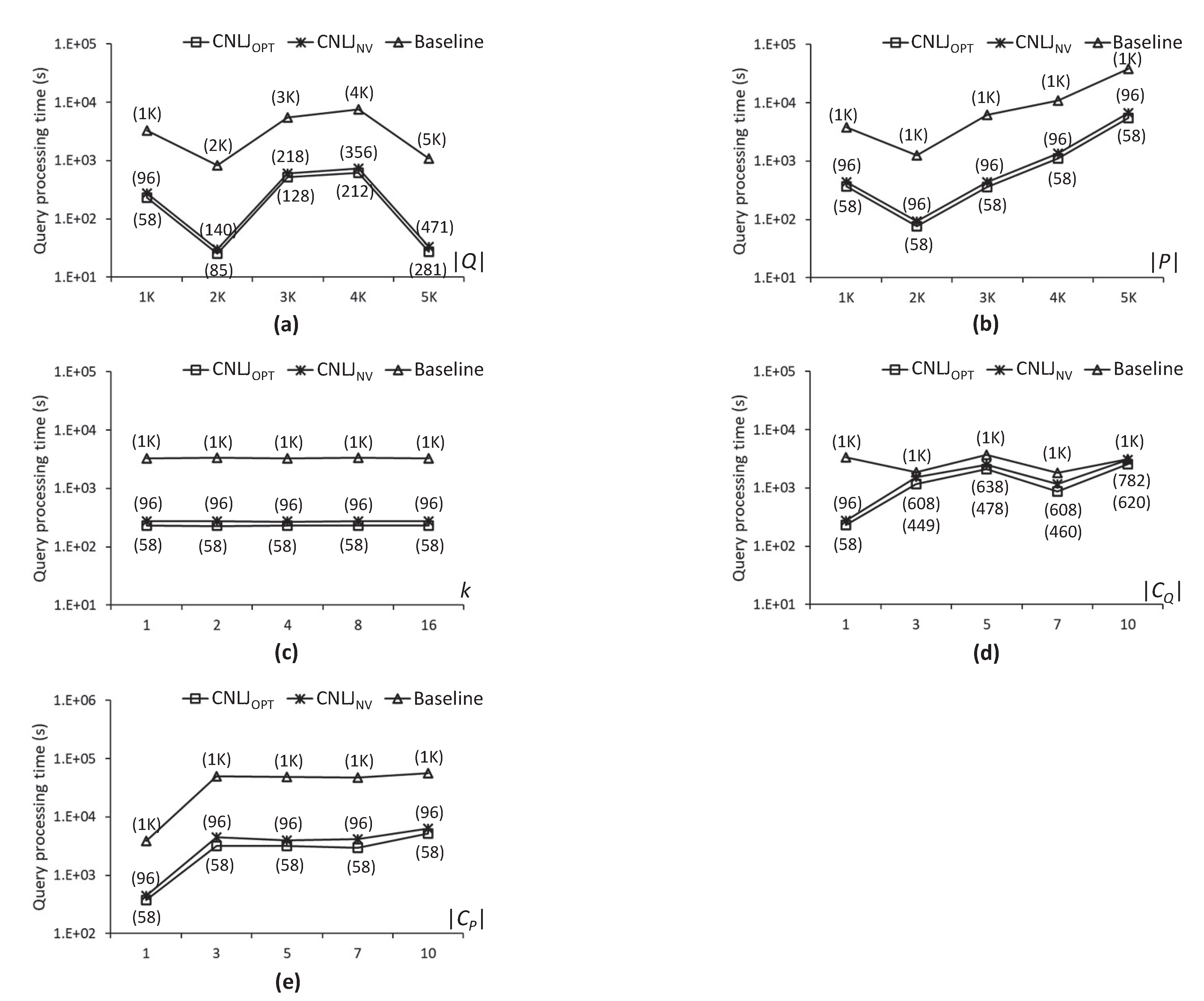
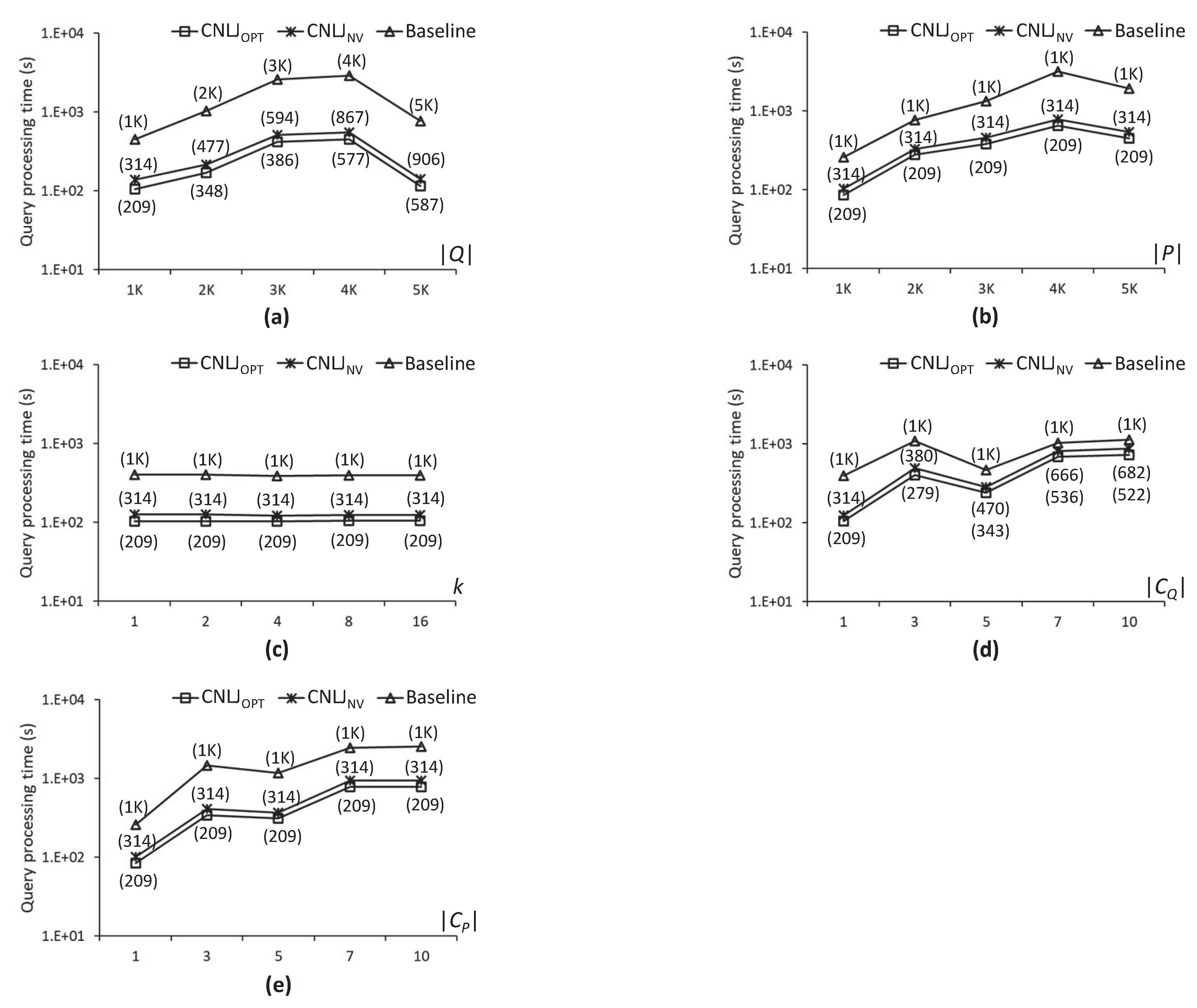
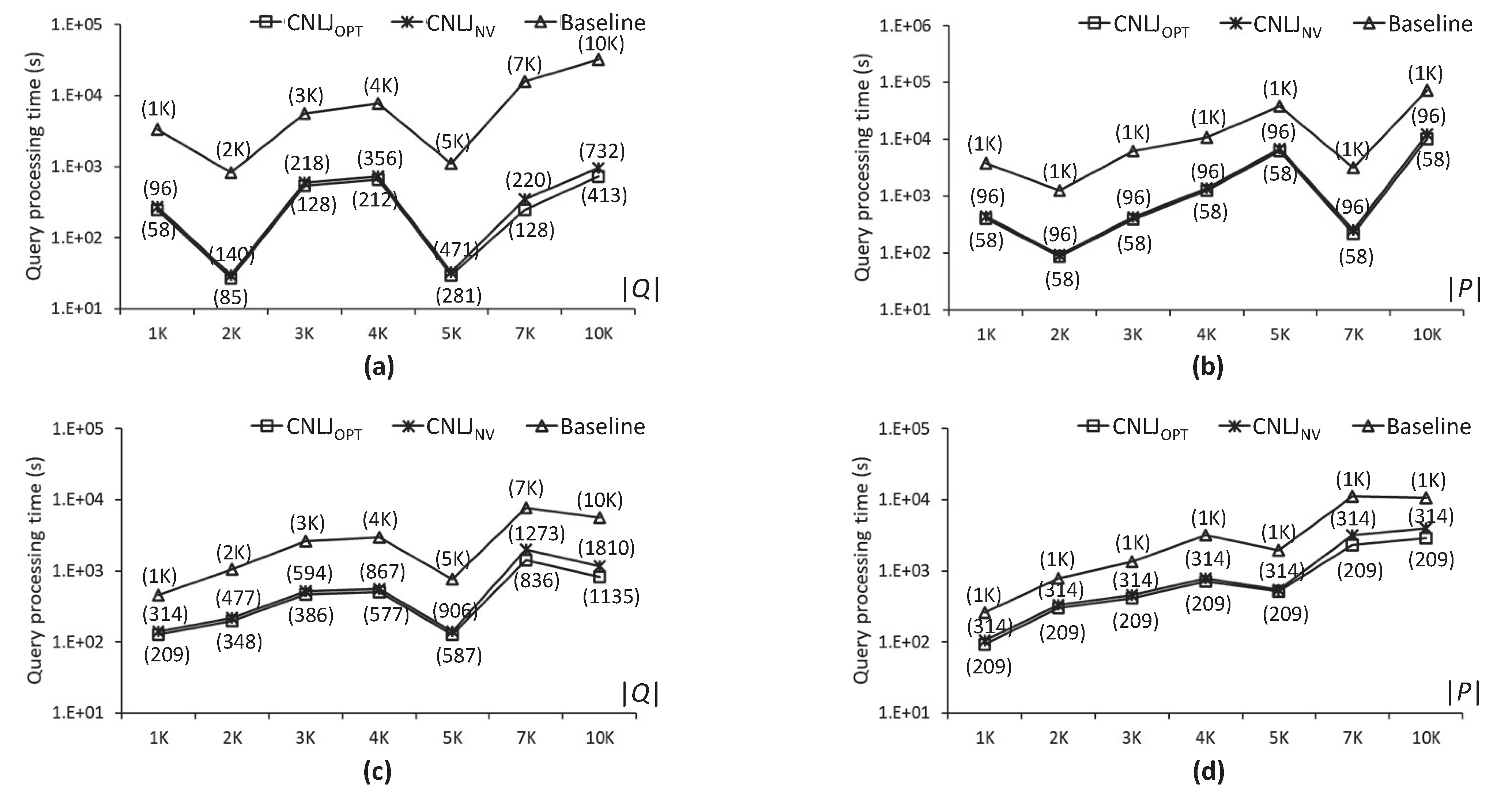
• An empirical study with various setups was conducted to demonstrate the superiority and scalability of the CNLJ algorithm. The CNLJ algorithm outperforms the conventional join algorithms by up to 50.8 times according to the results.

The remainder of this paper is organized as follows: Section 2 reviews related research and provides some background knowledge. Section 3 describes the clustering of query points (data points) and the computing of the maximum and minimum distances between a border point and a data cluster. Section 4 presents the CNLJ algorithm for rapidly evaluating kFN join queries in spatial networks. Section 5 presents the results of experiments using the CNLJ and conventional join algorithms with different setups. Finally, the conclusions of this study are discussed in Section 6.

2. Background

Section 2.1 presents related works and Section 2.2 defines the terms and notations used in this study.

2.1. Related Work

Many studies have considered spatial queries based on the farthest neighbor (FN) search [6,7,8,9,10,11,13,14,17,18,19,20]. Korn and Muthukrishnan [21] pioneered the concept of a reverse farthest neighbor (RFN) query to obtain the weak influence set. Given a set of data points P and a query point q, the RFN query retrieves a set of data points $p\in P$ such that q is their farthest neighbor among all points in $P\bigcup \left\{q\right\}$. This is the monochromatic RFN (MRFN) query [8,9,13,14,19]. Another version of the RFN query is the bichromatic reverse farthest neighbor (BRFN) query [10,13,14,22]. Given a set of data points P, a set of query points Q, and a query point q in Q, the BRFN query retrieves a set of data points p in P such that q is the farthest neighbor of p among all query points in Q. Many studies have been conducted to process RFN queries for the Euclidean space [8,9,14,19,22] and for spatial networks [10,13]. Yao et al. [14] proposed progressive farthest cell and convex hull farthest cell algorithms to answer RFN queries using an R-tree [23,24]. A solution to answer reverse kFN queries in the Euclidean space was presented for arbitrary values of k [22]. Liu et al. [19] proposed the concept of group RkFN query in the obstacle space and presented a query optimization algorithm based on the Voronoi graph. Tran et al. [10] proposed a solution for RFN queries and RkFN queries in road networks by using Voronoi-diagram-related attributes and Dijkstra’s algorithm. Xu et al. [13] presented efficient algorithms based on landmarks and hierarchical partitioning to process monochromatic and bichromatic RFN queries in spatial networks. The approximate version of the problem, known as the c-approximate farthest neighbor (c-AFN) search, has been actively studied due to the difficulty in designing an efficient method for exact FN search in high-dimensional space [6,17,18,25]. Huang et al. [18,25] introduced a new concept of reverse locality-sensitive hashing (LSH) family and developed reverse query-aware LSH functions. They proposed two hashing schemes for high-dimensional c-AFN search over external memory. Liu et al. [17] developed an approximate algorithm with a theoretical guarantee for high-dimensional c-AFN search over external memory. Curtin et al. [6] proposed an algorithm with an absolute approximation guarantee for the FN search in the high-dimensional space. To estimate the difficulty of the FN search problem, an information-theoretical measure of hardness was presented [6]. Farthest dominated location (FDL) queries were proposed in [26]. An FDL query retrieves the location $s\in L$ such that the distance to its nearest dominating object in P is maximized given a set of data points P with spatial and nonspatial attributes, a set L of candidate locations, and a design competence vector $\mathrm{\Psi }$ for L. Gao et al. [7] studied aggregate k-farthest neighbor (AkFN) queries that are defined by aggregation functions, such as min, max, and sum, and presented the MB and BF algorithms based on the R tree [23,24]. An AkFN query retrieves the k data points in P with the largest aggregate distances to all query points in Q given a set of data points P and a set of query points Q. In spatial networks, effective solutions to AkFN queries were proposed [11].

Due to the differences in the properties between the shortest path distance and the Euclidean distance, existing solutions based on the Euclidean space cannot be used directly to answer kFN join queries in spatial networks. The existing solutions for nearest neighbor search [27,28,29] cannot readily be used to address the farthest neighbor search problems due to the different distance properties between farness and nearness. Although the group computation of spatial queries has received considerable attention [19,27,30,31,32,33,34], group computation has not been applied to kFN join queries for spatial networks. To efficiently process kFN join queries in spatial networks, new sophisticated algorithms must be developed. First, the kFN join is a costly operation by definition. Second, farthest neighbor search is more difficult than nearest neighbor search. Finally, designing index structures that effectively support the FN search for spatial networks is difficult. In terms of the space domain, query type, and data type,

Table 1. Classification of related work.

References	Space Domain	Query Type	Data Type
[8,9,14,19]	Euclidean space	RkFN search	Monochromatic
[14,22]	Euclidean space	RkFN search	Bichromatic
[6,9,17,18,20,25]	Euclidean space	kFN search
[7]	Euclidean space	AkFN search
[26]	Euclidean space	FDL search
[13]	Spatial network	RkFN search	Monochromatic
[10,13]	Spatial network	RkFN search	Bichromatic
[35]	Spatial network	kFN search
[11]	Spatial network	AkFN search
This study	Spatial network	kFN join

compares our problem scenario to existing studies.

2.2. Notation and Formal Problem Description

Query and data points are placed in a spatial network G and these points represent points of interest (POIs), as shown in Figure 1. Given two points q and p, $dist(q,p)$ is the length of the shortest path between q and p in G.

Table 2. Symbols used in this paper and their meanings.

Symbol	Definition
k	Number of requested FNs
Q and q	A set Q of query points and query point q in Q, respectively
P and p	A set P of data points and data point p in P, respectively
$\overline{v_l{v_{l+1}\cdots v}_m}$	Vertex sequence where $v_l$ and $v_m$ are either an intersection vertex or a terminal vertex and the other vertices, $v_{l+1},\cdots {,v}_{m-1}$, are intermediate vertices
$\overline{q_i{q}_{i+1}{\cdots q}_j}$	Query segment connecting query points $q_i,q_{i+1},\cdots ,q_j$ in a vertex sequence (in short, $\overline{q_i{q}_j}$)
$\overline{p_l{p}_{l+1}{\cdots p}_m}$	Data segment connecting data points $p_l,p_{l+1},\cdots ,p_m$ in a vertex sequence (in short, $\overline{p_l{p}_m}$)
$\overline{Q_C}$ and $\overline{P_C}$	Set of query segments and set of data segments, respectively
$\overline{Q}$ and $\overline{P}$	Set of query clusters and set of data clusters, respectively
$B\left(\overline{Q_C}\right)$ and $B\left(\overline{P_C}\right)$	Sets of border points of $\overline{Q_C}$ and $\overline{P_C}$, respectively
$b_q$ and $b_p$	Border points of $\overline{Q_C}$ and $\overline{P_C}$, respectively
$\mathrm{\Omega }\left(q\right)$	Set of k data points farthest from a query point q
$dist(q,p)$	Length of the shortest path connecting points q and p
$len\left(\overline{qp}\right)$	Length of the segment $\overline{qp}$

summarizes the symbols used in this study.

Definition 1.

kFN search [6,7,8,9,10,11,13,14]. Given a positive integer k, a query point q, and a set P of data points, the query point q returns a set of k data points, denoted as $\mathrm{\Omega }\left(q\right)$, such that $dist(q,p^{+})\ge dist(q,p^{-})$ holds for $\forall p^{+}\in \mathrm{\Omega }\left(q\right)$ and $\forall p^{-}\in P-\mathrm{\Omega }\left(q\right)$.

Definition 2.

kFN join. Given a positive integer k, a set of query points Q, and a set of data points P, the kFN join query, denoted as $Q{⋉}_{kFN}P$, returns ordered pairs of each query point q in Q and a set of k data points farthest from q. For simplicity, $Q{⋉}_{kFN}P$ is abbreviated to $Q⋉P$, which is formally defined by $Q⋉P=\left\{〈q,\mathrm{\Omega }\left(q\right)〉\right|\forall q\in Q\}$. Note that the kFN joins are not commutative, i.e., $Q⋉P\ne P⋉Q$.

Definition 3.

Spatial network [32,33,36,37,38]. A weighted undirected graph $G=〈V,E,W〉$ is used to represent a spatial network, where V, E, and W represent the vertex set, edge set, and edge distance matrix, respectively. Each edge has a non-negative weight that indicates the network distance.

Definition 4.

Intersection, intermediate, and terminal vertices. Vertices can be divided into three categories based on their degree: (1) If the degree of a vertex is larger than or equal to 3, the vertex is referred to as an intersection vertex. (2) If the degree is 2, the vertex is an intermediate vertex. (3) If the degree is 1, the vertex is a terminal vertex.

Definition 5.

Vertex sequence, query segment, and data segment. A vertex sequence $\overline{v_l{v_{l+1}\cdots v}_m}$ denotes a path between two vertices, $v_l$ and $v_m$, such that $v_l$ and $v_m$ are either an intersection vertex or a terminal vertex, and the other vertices in the path, $v_{l+1},\cdots ,v_{m-1}$, are intermediate vertices. A query segment $\overline{q_i{q}_{i+1}\cdots q_j}$ denotes a line segment connecting query points $q_i,q_{i+1},\cdots ,q_j$ and a data segment $\overline{p_l{p}_{l+1}\cdots p_m}$ denotes a line segment connecting data points $p_l,p_{l+1},\cdots ,p_m$. For simplicity, $\overline{q_i{q}_j}$ and $\overline{p_l{p}_m}$ are abbreviated to $\overline{q_i{q}_{i+1}\cdots q_j}$ and $\overline{p_l{p}_{l+1}\cdots p_m}$, respectively, to reduce confusion.

3. Clustering Points and Computing Distances

In Section 3.1, we group query points (data points) by using the spatial network connection. We calculate the maximum and minimum distances between a border point and a data cluster in Section 3.2.

3.1. Clustering Query and Data Points Using Spatial Network Connection

Figure 2 illustrates an example of the kFN join $Q⋉P$, where $k=2$, $Q=\{q_1,q_2,q_3,q_4\}$, and $P=\{p_1,p_2,\cdots ,p_6\}$ are given. The example kFN join query requires that each query point q in Q finds two data points farthest from q.

Figure 3 shows an example of the two-step clustering method to group nearby query points into query clusters. A query segment is created in the first step by connecting query points in a vertex sequence. In Figure 3a, query points $q_1$ and $q_2$ in a vertex sequence $\overline{q_1{q}_2{v}_2}$ are connected to become $\overline{q_1{q}_2}$. Thus, three query segments $\overline{q_1{q}_2}$, $q_3$, and $q_4$ are generated, as shown in Figure 3a. In the second step, an intersection vertex is used to connect adjacent query segments to form a query cluster. In Figure 3b, the intersection vertex $q_1$ connects two query segments $\overline{q_1{q}_2}$ and $q_4$. Similarly, $q_3$ and $q_4$ are linked by the intersection vertex $v_1$. Finally, $\overline{q_1{q}_2}$ and $q_3$ are linked by the intersection vertex $v_2$. As a result, three query segments $\overline{q_1{q}_2}$, $q_3$, and $q_4$ are linked to form a query cluster $\{\overline{q_1{q_{2}v}_2},\overline{q_1{q_{4}v}_1},\overline{v_1{q}_3{v}_2}\}$. Note that a query cluster is a set of query segments. Naturally, a set of query points $Q=\{q_1,q_2,q_3,q_4\}$ is converted into a set of query clusters $\overline{Q}=\left\{\{\overline{q_1{q_{2}v}_2},\overline{q_1{q_{4}v}_1},\overline{v_1{q}_3{v}_2}\}\right\}$. Let us define a border point for a query cluster $\overline{Q_C}$. When a query cluster $\overline{Q_C}$ and its nonquery cluster $G-\overline{Q_C}$ meet at a point, that point is referred to as the border point of $\overline{Q_C}$. In this example, three border points $q_1$, $v_1$, and $v_2$ are found for $\overline{Q_C}=\{\overline{q_1{q_{2}v}_2},\overline{q_1{q_{4}v}_1},\overline{v_1{q}_3{v}_2}\}$. Thus, a set of border points of $\overline{Q_C}$ is represented by $B\left(\overline{Q_C}\right)=\{q_1,v_1,v_2\}$.

Figure 4 shows an example of a two-step clustering method to group neighboring data points into data clusters. Notably, the query and data points are clustered using the same two-step method. In the first step, data points $p_1$, $p_2$, and $p_3$ in a vertex sequence $\overline{v_1{p}_2{v}_3}$ are connected to become a data segment $\overline{p_1{p}_2{p}_3}$. Similarly, data points $p_4$ and $p_5$ in a vertex sequence $\overline{p_5{p}_4{q}_1}$ are linked to form a data segment $\overline{p_4{p}_5}$. As a result, three data segments $\overline{p_1{p}_2{p}_3}$, $\overline{p_4{p}_5}$, and $p_6$ are generated, as illustrated in Figure 4a. In the second step, two data segments $\overline{p_4{p}_5}$ and $p_6$ are joined by an intersection vertex $p_5$ to form a data cluster $\{\overline{p_4{p}_5},\overline{p_5{p}_6}\}$. As a result, a set of data points $P=\{p_1,p_2,\cdots ,p_6\}$ is transformed into a set of data clusters $\overline{P}=\{\left\{\overline{p_1{p}_2{p}_3}\right\},\{\overline{p_4{p}_5},\overline{p_5{p}_6}\}\}$.

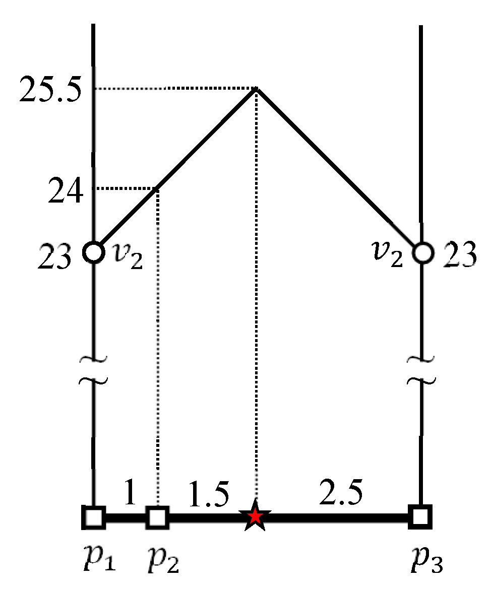
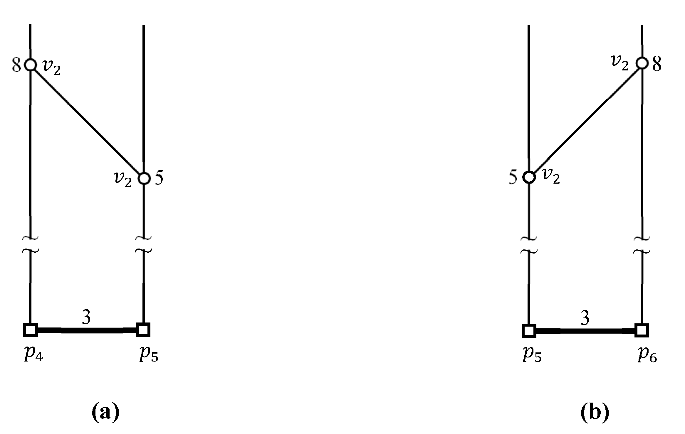
3.2. Computing Maximum and Minimum Distances from a Border Point to a Data Cluster

The maximum and minimum distances between a border point $b_q$ and a data cluster $\overline{P_C}$ are computed in this section. The minimum and maximum distances between $b_q$ and $\overline{P_C}$ are formally defined by $mindist(b_q,\overline{P_C})=min\left\{dist(b_q,p)\right|p\in \overline{P_C}\}$ and $maxdist(b_q,\overline{P_C})=max\left\{dist(b_q,p)\right|p\in \overline{P_C}\}$, respectively. The minimum distance between $b_q$ and $\overline{P_C}$ can be easily calculated by $mindist(b_q,\overline{P_C})=min\left\{dist(b_q,b_p)\right|b_p\in B\left(\overline{P_C}\right)\}$ where $b_p$ is a border point of a data cluster $\overline{P_C}$. The maximum distance between $b_q$ and $\overline{P_C}$ can be represented by $maxdist(b_q,\overline{P_C})=max\left\{maxdist(b_q,\overline{p_l{p}_m})\right|\overline{p_l{p}_m}\in \overline{P_C}\}$ where $maxdist(b_q,\overline{p_l{p}_m})$ is the maximum distance between $b_q$ and a data segment $\overline{p_l{p}_m}$ in $\overline{P_C}$.

An example is used to illustrate how to compute the maximum and minimum distances between a border point $b_q$ and a data cluster $\overline{P_C}$. Note that the example kFN join query has three border points and two data clusters, i.e., $B\left(\overline{Q_C}\right)=\{q_1,v_1,v_2\}$ and $\overline{P}=\{\left\{\overline{p_1{p}_2{p}_3}\right\},\{\overline{p_4{p}_5},\overline{p_5{p}_6}\}\}$. In this section, the maximum and minimum distances between $b_q$ and $\overline{P_C}$ are computed, where $b_q\in \{q_1,v_1,v_2\}$ and $\overline{P_C}\in \{\left\{\overline{p_1{p}_2{p}_3}\right\},\{\overline{p_4{p}_5},\overline{p_5{p}_6}\}\}$. Note that computations of $maxdist(q_1,\left\{\overline{p_1{p}_2{p}_3}\right\})$, $maxdist(q_1,$$\{\overline{p_4{p}_5},\overline{p_5{p}_6}\})$, $maxdist(v_1,$$\left\{\overline{p_1{p}_2{p}_3}\right\})$, $maxdist(v_1,$$\{\overline{p_4{p}_5},\overline{p_5{p}_6}\})$, $maxdist(v_2,$$\left\{\overline{p_1{p}_2{p}_3}\right\})$, and $maxdist(v_2,$$\{\overline{p_4{p}_5},\overline{p_5{p}_6}\})$ are illustrated in Figure 5, Figure 6, Figure 7, Figure 8, Figure 9 and Figure 10, respectively.

Figure 5 illustrates the computation of $maxdist(q_1,$$\left\{\overline{p_1{p}_2{p}_3}\right\})$. First, the distances from $q_1$ to the endpoints $p_1$ and $p_3$ of $\overline{p_1{p}_2{p}_3}$ evaluate to $dist(q_1,p_1)=24$ and $dist(q_1,p_3)=27$, respectively. Consider a point p in $\overline{p_1{p}_2{p}_3}$. Because p lies in $\overline{p_1{p}_2{p}_3}$, whose length is $len\left(\overline{p_1{p}_2{p}_3}\right)=5$, the distance between $q_1$ and p is computed by $dist(q_1,p)=$$min$$\{dist(q_1,p_1)+len\left(\overline{p_{1}p}\right),dist(q_1,p_3)+len\left(\overline{p_{3}p}\right)\}$ $=min\{24+len\left(\overline{p_{1}p}\right),27+len\left(\overline{p_{3}p}\right)\}$. Let $x=len\left(\overline{p_{1}p}\right)$ for $0\le x\le 5$. Then, we have $len\left(\overline{p_{3}p}\right)=5-x$ because $len\left(\overline{p_{1}p}\right)+len\left(\overline{p_{3}p}\right)=5$. We can rewrite $dist(q_1,p)=min\{24+x,27+(5-x)\}$ for $0\le x\le 5$. As shown in Figure 5, the maximum and minimum distances between $q_1$ and $\left\{\overline{p_1{p}_2{p}_3}\right\}$ is $maxdist(q_1,\left\{\overline{p_1{p}_2{p}_3}\right\})=28$ and $mindist(q_1,$$\left\{\overline{p_1{p}_2{p}_3}\right\})=24$, respectively. For convenience, the star symbol (★) in Figure 5 is marked to indicate $maxdist(q_1,\left\{\overline{p_1{p}_2{p}_3}\right\})=28$.

The maximum distance between a border point $q_1$ and a data cluster $\{\overline{p_4{p}_5},\overline{p_5{p}_6}\}$ is represented by $maxdist(q_1,\{\overline{p_4{p}_5},\overline{p_5{p}_6}\})$$=max\{maxdist(q_1,\overline{p_4{p}_5}),$$maxdist(q_1,\overline{p_5{p}_6})\}$. The computations of $maxdist(q_1,\overline{p_4{p}_5})$ and $maxdist(q_1,\overline{p_5{p}_6})$ are illustrated in Figure 6a,b, respectively. The distances from $q_1$ to the endpoints $p_4$ and $p_5$ are $dist(q_1,p_4)=5$ and $dist(q_1,p_5)=8$, respectively. The maximum and minimum distances from $q_1$ to $\overline{p_4{p}_5}$ are shown in Figure 6a as $maxdist(q_1,\overline{p_4{p}_5})=8$ and $mindist(q_1,\overline{p_4{p}_5})=5$, respectively. The distances from $q_1$ to the endpoints $p_5$ and $p_6$ of $\overline{p_5{p}_6}$ are $dist(q_1,p_5)=8$ and $dist(q_1,p_6)=11$, respectively. The maximum and minimum distances from $q_1$ to $\overline{p_5{p}_6}$ are calculated to be $maxdist(q_1,\overline{p_5{p}_6})=11$ and $mindist(q_1,\overline{p_5{p}_6})=8$, respectively, as shown in Figure 6b. Therefore, the maximum and minimum distances between $q_1$ and $\{\overline{p_4{p}_5},\overline{p_5{p}_6}\}$ are $maxdist(q_1,\{\overline{p_4{p}_5},\overline{p_5{p}_6}\})=11$ and $mindist(q_1,\{\overline{p_4{p}_5},\overline{p_5{p}_6}\})=5$, respectively.

Figure 7 illustrates the computation of $maxdist(v_1,$$\left\{\overline{p_1{p}_2{p}_3}\right\})$ and $mindist(v_1,$$\left\{\overline{p_1{p}_2{p}_3}\right\})$. The distances from $v_1$ to the endpoints $p_1$ and $p_3$ of $\overline{p_1{p}_2{p}_3}$ are $dist(v_1,p_1)=19$ and $dist(v_1,p_3)=24$, respectively. Thus, the maximum and minimum distances between $v_1$ and $\left\{\overline{p_1{p}_2{p}_3}\right\}$ are $maxdist(v_1,\left\{\overline{p_1{p}_2{p}_3}\right\})=24$ and $mindist(v_1,\left\{\overline{p_1{p}_2{p}_3}\right\})=19$, respectively.

Figure 8 illustrates the computation of $maxdist(v_1,$$\{\overline{p_4{p}_5},\overline{p_5{p}_6}\})$ and $mindist(v_1,$$\{\overline{p_4{p}_5},\overline{p_5{p}_6}\})$. The maximum distance between $v_1$ and $\{\overline{p_4{p}_5},\overline{p_5{p}_6}\}$ is computed by $maxdist(v_1,\{\overline{p_4{p}_5},\overline{p_5{p}_6}\})=max\{maxdist(v_1,\overline{p_4{p}_5}),$$maxdist(v_1,\overline{p_5{p}_6})\}$. The computations of $maxdist(v_1,\overline{p_4{p}_5})$ and $maxdist(v_1,\overline{p_5{p}_6})$ are illustrated in Figure 8a,b, respectively. The distances from $v_1$ to the endpoints $p_4$ and $p_5$ of $\overline{p_4{p}_5}$ are $dist(v_1,p_4)=10$ and $dist(v_1,p_5)=9$, respectively. Thus, the maximum and minimum distances between $v_1$ and $\overline{p_4{p}_5}$ are $maxdist(v_1,\overline{p_4{p}_5})=11$ and $mindist(v_1,\overline{p_4{p}_5})=9$, respectively, as shown in Figure 8a, where the star symbol (★) is marked to indicate $maxdist(v_1,\overline{p_4{p}_5})=11$. The distances from $v_1$ to the endpoints $p_5$ and $p_6$ of $\overline{p_5{p}_6}$ are $dist(v_1,p_5)=9$ and $dist(v_1,p_6)=12$, respectively. As shown in Figure 8b, the maximum and minimum distances between $v_1$ and $\overline{p_5{p}_6}$ are $maxdist(v_1,\overline{p_5{p}_6})=12$ and $mindist(v_1,\overline{p_5{p}_6})=9$, respectively. Thus, the maximum and minimum distances between $v_1$ and $\{\overline{p_4{p}_5},\overline{p_5{p}_6}\}$ are $maxdist(v_1,\{\overline{p_4{p}_5},\overline{p_5{p}_6}\})=12$ and $mindist(v_1,\{\overline{p_4{p}_5},\overline{p_5{p}_6}\})=9$, respectively.

Figure 9 illustrates the computation of $maxdist(v_2,$$\left\{\overline{p_1{p}_2{p}_3}\right\})$ and $mindist(v_2,$$\left\{\overline{p_1{p}_2{p}_3}\right\})$. The distances from $v_2$ to the endpoints $p_1$ and $p_3$ of $\overline{p_1{p}_2{p}_3}$ are $dist(v_2,p_1)=dist(v_2,p_3)=23$, respectively. Thus, the maximum and minimum distances between $v_2$ and $\left\{\overline{p_1{p}_2{p}_3}\right\}$ are $maxdist(v_2,\left\{\overline{p_1{p}_2{p}_3}\right\})=25.5$ and $mindist(v_2,\left\{\overline{p_1{p}_2{p}_3}\right\})=23$, respectively. Note that the star symbol (★) in Figure 9 is marked to indicate $maxdist(v_2,\left\{\overline{p_1{p}_2{p}_3}\right\})=25.5$.

Figure 10 illustrates the computation of $maxdist(v_2,$$\{\overline{p_4{p}_5},\overline{p_5{p}_6}\})$ and $mindist(v_2,$$\{\overline{p_4{p}_5},\overline{p_5{p}_6}\})$. The maximum distance between $v_2$ and $\{\overline{p_4{p}_5},\overline{p_5{p}_6}\}$ is computed by $maxdist(v_2,\{\overline{p_4{p}_5},\overline{p_5{p}_6}\})=max\{maxdist(v_2,\overline{p_4{p}_5}),$$maxdist(v_2,\overline{p_5{p}_6})\}$. The computations of $maxdist(v_2,\overline{p_4{p}_5})$ and $maxdist(v_2,\overline{p_5{p}_6})$ are illustrated in Figure 10a,b, respectively. The distances from $v_2$ to the endpoints $p_4$ and $p_5$ of $\overline{p_4{p}_5}$ are $dist(v_2,p_4)=8$ and $dist(v_2,p_5)=5$, respectively. Thus, the maximum and minimum distances between $v_2$ and $\overline{p_4{p}_5}$ are $maxdist(v_2,\overline{p_4{p}_5})=8$ and $mindist(v_2,\overline{p_4{p}_5})=5$, respectively, as shown in Figure 10a. The distances from $v_2$ to the endpoints $p_5$ and $p_6$ of $\overline{p_5{p}_6}$ are $dist(v_2,p_5)=5$ and $dist(v_2,p_6)=8$, respectively. Thus, the maximum and minimum distances between $v_2$ and $\overline{p_5{p}_6}$ are $maxdist(v_2,\overline{p_5{p}_6})=8$ and $mindist(v_2,\overline{p_5{p}_6})=5$, respectively, as shown in Figure 10b. Thus, the maximum and minimum distances between $v_2$ and $\{\overline{p_4{p}_5},\overline{p_5{p}_6}\}$ are $maxdist(v_2,\{\overline{p_4{p}_5},\overline{p_5{p}_6}\})=8$ and $mindist(v_2,\{\overline{p_4{p}_5},\overline{p_5{p}_6}\})=5$, respectively.

Table 3. Maximum and minimum distances between border points and data clusters.

${\mathit{b}}_{\mathit{q}}$	$\left\{\overline{{\mathit{p}}_1{\mathit{p}}_2{\mathit{p}}_3}\right\}$	$\{\overline{{\mathit{p}}_4{\mathit{p}}_5},\overline{{\mathit{p}}_5{\mathit{p}}_6}\}$
$q_1$	$maxdist(q_1,\left\{\overline{p_1{p}_2{p}_3}\right\})=28$	$maxdist(q_1,\{\overline{p_4{p}_5},\overline{p_5{p}_6}\})=11$
	$mindist(q_1,\left\{\overline{p_1{p}_2{p}_3}\right\})=24$	$mindist(q_1,\{\overline{p_4{p}_5},\overline{p_5{p}_6}\})=5$
$v_1$	$maxdist(v_1,\left\{\overline{p_1{p}_2{p}_3}\right\})=24$	$maxdist(v_1,\{\overline{p_4{p}_5},\overline{p_5{p}_6}\})=12$
	$mindist(v_1,\left\{\overline{p_1{p}_2{p}_3}\right\})=19$	$mindist(v_1,\{\overline{p_4{p}_5},\overline{p_5{p}_6}\})=9$
$v_2$	$maxdist(v_2,\left\{\overline{p_1{p}_2{p}_3}\right\})=25.5$	$maxdist(v_2,\{\overline{p_4{p}_5},\overline{p_5{p}_6}\})=8$
	$mindist(v_2,\left\{\overline{p_1{p}_2{p}_3}\right\})=23$	$mindist(v_2,\{\overline{p_4{p}_5},\overline{p_5{p}_6}\})=5$

summarizes the maximum and minimum distances between the border points in $B\left(\overline{Q_C}\right)$ and the data clusters in $\overline{P}$.

4. Cluster Nested Loop Join Algorithm for Spatial Networks

The CNLJ algorithm is described in Section 4.1. Section 4.2 evaluates k FNs queries at the border points of query clusters. Finally, the example k FNs join query is evaluated in Section 4.3.

4.1. Cluster Nested Loop Join Algorithm

The CNLJ algorithm is described in Algorithm 1, which involves two steps. The two-step clustering method (lines 2–4), which is described in Section 3.1, is used to group nearby query points (data points) into query clusters (data clusters) in the first step. In the second step, the kFN join is performed for each query cluster in $\overline{Q}$ (lines 5–8). Finally, the kFN join result $\mathrm{\Omega }\left(Q\right)$ is returned to a query user when the kFN join is complete for each query cluster in $\overline{Q}$ (line 9).

Algorithm 1 CNLJ($k,Q,P$).

Input:k: number of FNs for q, Q: set of query points, and P: set of data points  Output:$\mathrm{\Omega }\left(Q\right)$: Set of ordered pairs of each query point q in Q and a set of k FNs for q, i.e., $\mathrm{\Omega }\left(Q\right)=\left\{〈q,\mathrm{\Omega }\left(q\right)〉\right|q\in Q\}$.  1: $\mathrm{\Omega }\left(Q\right)\leftarrow \varnothing$                             // The result set $\mathrm{\Omega }\left(Q\right)$ is initialized to the empty set.  2: // Step 1: Query and data points are clustered, which is presented in Section 3.1.  3: $\overline{Q}\leftarrow two\_step\_clustering\left(Q\right)$                  // Query points are grouped into query clusters.  4: $\overline{P}\leftarrow two\_step\_clustering\left(P\right)$                   // Data points are grouped into data clusters.  5: // Step 2: The kFN join is performed for each query cluster in $\overline{Q}$, which is presented in Algorithm 2.  6: for each query cluster $\overline{Q_C}\in \overline{Q}$ do  7:    $\mathrm{\Omega }\left(\overline{Q_C}\right)\leftarrow kFN\_join(k,\overline{Q_C},\overline{P})$                         // $\mathrm{\Omega }\left(\overline{Q_C}\right)=\left\{〈q,\mathrm{\Omega }\left(q\right)〉\right|q\in \overline{Q_C}\}$.  8:    $\mathrm{\Omega }\left(Q\right)\leftarrow \mathrm{\Omega }\left(Q\right)\cup \mathrm{\Omega }\left(\overline{Q_C}\right)$                      // the kFN join result for $\overline{Q_C}$ is added to $\mathrm{\Omega }\left(Q\right)$.  9: return$\mathrm{\Omega }\left(Q\right)$                // $\mathrm{\Omega }\left(Q\right)$ is returned once the kFN join for every query cluster in $\overline{Q}$ is complete.

Algorithm 2 describes the kFN join algorithm for a query cluster $\overline{Q_C}$. First, kFN queries are evaluated at the border points of $\overline{Q_C}$ to collect the candidate data points for query points in $\overline{Q_C}$ (lines 4–7), which is described in Algorithm 3. Then, each query point q in $\overline{Q_C}$ retrieves the kFNs for q among the candidate data points in $\mathrm{\Omega }\left(B\left(\overline{Q_C}\right)\right)$ (lines 8–11), which is detailed in Algorithm 4. Finally, the kFN join result $\mathrm{\Omega }\left(\overline{Q_C}\right)$ for query points in $\overline{Q_C}$ is returned after each query point q in $\overline{Q_C}$ retrieves the kFNs for q from the candidate data points (line 12).

Algorithm 2$kFN\_join(k,\overline{Q_C},\overline{P})$.

Input:k: number of FNs for q, $\overline{Q_C}$: query cluster, and $\overline{P}$: set of data clusters  Output:$\mathrm{\Omega }\left(\overline{Q_C}\right)$: Set of ordered pairs of each query point q in $\overline{Q_C}$ and a set of k FNs for q, i.e., $\mathrm{\Omega }\left(\overline{Q_C}\right)=\left\{〈q,\mathrm{\Omega }\left(q\right)〉\right|q\in \overline{Q_C}\}$  1: $\mathrm{\Omega }\left(\overline{Q_C}\right)\leftarrow \varnothing$                    // The result set for query points in $\overline{Q_C}$ is initialized to the empty set.  2: $\mathrm{\Omega }\left(B\left(\overline{Q_C}\right)\right)\leftarrow \varnothing$                        // Note that $\mathrm{\Omega }\left(B\left(\overline{Q_C}\right)\right)=\left\{〈b_q,\mathrm{\Omega }\left(b_q\right)〉\right|b_q\in B\left(\overline{Q_C}\right)\}$.  3: $l\leftarrow max\left\{dist(b_{q_i},b_{q_j})\right|b_{q_i},b_{q_j}\in B\left(\overline{Q_C}\right)\}$       // l indicates the maximum distance between border points in $\overline{Q_C}$.  4: // Step 1: kFN query is evaluated at each border point $b_q$ in $\overline{Q_C}$  5: for each border point $b_q\in B\left(\overline{Q_C}\right)$ do  6:    $\mathrm{\Omega }\left(b_q\right)\leftarrow find\_candidates(k,l,b_q,\overline{P})$       // kFN query is evaluated at $b_q$, which is detailed in Algorithm 3.  7:    $\mathrm{\Omega }\left(B\left(\overline{Q_C}\right)\right)\leftarrow \mathrm{\Omega }\left(B\left(\overline{Q_C}\right)\right)\cup \mathrm{\Omega }\left(b_q\right)$            // $\mathrm{\Omega }\left(B\left(\overline{Q_C}\right)\right)$ collects candidate data points for query points in $\overline{Q_C}$.  8: // Step 2: Each query point q retrieves k FNs among the candidate data points in $\mathrm{\Omega }\left(B\left(\overline{Q_C}\right)\right)$.  9: for each query point $q\in \overline{Q_C}$ do  10:    $\mathrm{\Omega }\left(q\right)\leftarrow retrieve\_kFN(k,q,\mathrm{\Omega }\left(B\left(\overline{Q_C}\right)\right))$          // $\mathrm{\Omega }\left(B\left(\overline{Q_C}\right)\right)$ is the set of candidate data points for q.  11:    $\mathrm{\Omega }\left(\overline{Q_C}\right)\leftarrow \mathrm{\Omega }\left(\overline{Q_C}\right)\cup \mathrm{\Omega }\left(q\right)$  12: return$\mathrm{\Omega }\left(\overline{Q_C}\right)$             // $\mathrm{\Omega }\left(\overline{Q_C}\right)$ is returned once the kFN search is performed for each query point in $\overline{Q_C}$.

Algorithm 3 describes the kFN query processing algorithm for finding candidate data points at a border point $b_q$ for a query cluster. Note that the kFN query result for $b_q$ includes candidate data points for query points in $\overline{Q_C}$. The set of kFNs for $b_q$, $\mathrm{\Omega }\left(b_q\right)$, is initialized to the empty set (line 1). The third argument l indicates the maximum distance between border points in $\overline{Q_C}$, i.e., $l\leftarrow max\left\{dist(b_{q_i},b_{q_j})\right|b_{q_i},b_{q_j}\in B\left(\overline{Q_C}\right)\}$. The sentinel distance is initialized to $sntl\_dist\leftarrow 0$ and determines whether a data point p is a candidate point for $\overline{Q_C}$. The maximum and minimum distances from $b_q$ to data clusters in $\overline{P}$ are computed, as described in Section 3.2. The data clusters are then sorted in decreasing order of their maximum distance to $b_q$. Naturally, the sorted data clusters are explored sequentially. If the maximum distance from $b_q$ to the data cluster $\overline{P_C}$ to be explored next is smaller than the sentinel distance, i.e., $maxdist(b_q,\overline{P_C})<sntl\_dist$, the remaining unexplored data clusters do not need to be considered because the data points in these data clusters can be candidate data points for no query point in $\overline{Q_C}$. Otherwise (i.e., $maxdist(b_q,\overline{P_C})\ge sntl\_dist$), each data point p in $\overline{P_C}$ needs to be examined to determine whether p is a candidate point for query points in $\overline{Q_C}$. For this, $dist(b_q,p)$ is computed. If $b_q$ is inside $\overline{P_C}$, then the distance from $b_q$ to p is simply computed using a graph search algorithm such as Dijkstra’s algorithm [39]. Otherwise (i.e., if $b_q$ is outside $\overline{P_C}$), the distance evaluates to $dist(b_q,p)\leftarrow min\{dist(b_q,b_p)+dist(b_p,p)|b_p\in B\left(\overline{P_C}\right)\}$. Note that $b_q$ is a border point of $\overline{Q_C}$ and $b_p$ is a border point of $\overline{P_C}$. This is because if $b_q$ is outside $\overline{P_C}$, the shortest path from $b_q$ to p should pass through a border point $b_p$ of $\overline{P_C}$, i.e., $b_q\to b_p\to p$. If $dist(b_q,p)\ge sntl\_dist$, then p is added to $\mathrm{\Omega }\left(b_q\right)$ as a candidate data point for $\overline{Q_C}$. Redundant data points p may be included in $\mathrm{\Omega }\left(b_q\right)$ and they should be removed from $\mathrm{\Omega }\left(b_q\right)$. Thus, each data point p in $\mathrm{\Omega }\left(b_q\right)$ is explored to verify that p is qualified to be a candidate data point, i.e., $dist(b_q,p)\ge sntl\_dist$. If p does not satisfy the qualification, it is removed from $\mathrm{\Omega }\left(b_q\right)$. Finally, if the maximum distance from $b_q$ to the data cluster $\overline{P_C}$ is smaller than the sentinel distance (lines 10–12) or if every data cluster is examined, the k FN query result for $b_q$, $\mathrm{\Omega }\left(b_q\right)$, is returned.

Algorithm 3$find\_candidates(k,l,b_q,\overline{P})$.

Input:k: number of FNs for q, l: maximum distance between border points in $\overline{Q_C}$, $b_q$: border point of $\overline{Q_C}$, and $\overline{P}$: set of data clusters  Output:$\mathrm{\Omega }\left(b_q\right)$: Set of k FNs for $b_q$  1: $\mathrm{\Omega }\left(b_q\right)\leftarrow \varnothing$                   // The set of k FNs for a border point $b_q$, $\mathrm{\Omega }\left(b_q\right)$, is initialized to the empty set.  2: $sntl\_dist\leftarrow 0$                          // t = The sentinel distance $sntl\_dist$ is initialized to 0.  3: // The maximum and minimum distances from $b_q$ to data clusters in $\overline{P}$ are computed as explained in Section 3.2.  4: for each data cluster $\overline{P_C}\in \overline{P}$ do  5:     compute $maxdist(b_q,\overline{P_C})$ and $mindist(b_q,\overline{P_C})$  6: // The data clusters in $\overline{P}$ are sorted in decreasing order of their maximum distance to $b_q$  7: $\overline{P}\leftarrow sort\_data\_clusters(\overline{P}$)                       // $\overline{P}$ contains the sorted data clusters for $b_q$.  8: // Data clusters are explored sequentially.  9: for each sorted data cluster $\overline{P_C}\in \overline{P}$ do  10:    if $maxdist(b_q,\overline{P_C})<sntl\_dist$ then  11:        // Note that $sntl\_dist$ is updated as shown in line 24.  12:      Go to line 26                    // This means that the other data clusters do not need to be explored.  13:    // Each data point p in $\overline{P_C}$ is sequentially explored to find k FNs for $b_q$.  14:    for each data point $p\in \overline{P_C}$ do  15:        // $dist(b_q,p)$ is computed using the following two cases. $b_q\in$$\overline{P_C}$ and $b_q\notin$$\overline{P_C}$.  16:      if $b_q$ is inside $\overline{P_C}$ then  17:         $dist(b_q,p)$ is simply computed using a graph search algorithm such as Dijkstra’s algorithm [39]  18:      else  19:         $dist(b_q,p)\leftarrow min\{dist(b_q,b_p)+dist(b_p,p)|b_p\in B\left(\overline{P_C}\right)\}$   // Note that the path from $b_q$ to p is $b_q\to b_p\to p$.  20:      // p is added to $\mathrm{\Omega }\left(b_q\right)$ if $dist(b_q,p)\ge sntl\_dist$.  21:      if $dist(b_q,p)\ge sntl\_dist$ then  22:         // $\mathrm{\Omega }\left(b_q\right)$ collects candidate data points for query points in $\overline{Q_C}$.  23:         $\mathrm{\Omega }\left(b_q\right)\leftarrow \mathrm{\Omega }\left(b_q\right)\cup \left\{p\right\}$                                  // p is added to $\mathrm{\Omega }\left(b_q\right)$.  24:         $sntl\_dist\leftarrow dist(b_q,p_{kth})-l$                         // $p_{kth}$ is the current kth FN of $b_q$.  25: // Redundant data points p are removed from $\mathrm{\Omega }\left(b_q\right)$ because they can be kFNs of no query point in $\overline{Q_C}$  26: for each data point $p\in \mathrm{\Omega }\left(b_q\right)$ do  27:    if $dist(b_q,p)<sntl\_dist$ then  28:        $\mathrm{\Omega }\left(b_q\right)\leftarrow \mathrm{\Omega }\left(b_q\right)-\left\{p\right\}$              // p is no candidate data point for $\overline{Q_C}$ and it is removed from $\mathrm{\Omega }\left(b_q\right)$.  29: return$\mathrm{\Omega }\left(b_q\right)$              // $\mathrm{\Omega }\left(b_q\right)$ is returned after candidate data points are collected for query points in $\overline{Q_C}$.

Algorithm 4 describes that a query point q in $\overline{Q_C}$ retrieves k FNs for q among candidate data points in $\mathrm{\Omega }\left(B\left(\overline{Q_C}\right)\right)$. First, $\mathrm{\Omega }\left(q\right)$ is initialized to the empty set. The distance between q and a candidate data point p is computed using the following two cases: $p\in$$\overline{Q_C}$ and $p\notin$$\overline{Q_C}$. If p is inside $\overline{Q_C}$, i.e., $p\in$$\overline{Q_C}$, then the distance from q to p is simply computed using a graph search algorithm [39]. Otherwise (i.e., $p\notin$$\overline{Q_C}$), the distance evaluates to $dist(q,p)\leftarrow min\{dist(q,b_q)+dist(b_q,p)|b_q\in B\left(\overline{Q_C}\right)\}$. This is because the shortest path from q to p should pass through a border point $b_q$ of $\overline{Q_C}$, i.e., $q\to b_q\to p$. When $dist(q,p)$ is computed, the following two conditions are checked to determine whether the data point p is added to $\mathrm{\Omega }\left(q\right)$: If the cardinality of $\mathrm{\Omega }\left(q\right)$ is smaller than k, i.e., $\left|\mathrm{\Omega }\right(q\left)\right|<k$, then p is simply added to $\mathrm{\Omega }\left(q\right)$. Furthermore, if p is farther from q than the current kth FN $p_{kth}$ of q, i.e., $dist(q,p)>dist(q,p_{kth})$, then p is added to $\mathrm{\Omega }\left(q\right)$ and $p_{kth}$ is removed from $\mathrm{\Omega }\left(q\right)$. Finally, when exploration of every candidate data point is complete, the kFN query result for q, $\mathrm{\Omega }\left(q\right)$, is returned.

Algorithm 4$retrieve\_kFN(k,q,\mathrm{\Omega }\left(B\left(\overline{Q_C}\right)\right))$.

Input:k: number of FNs for q, q: query point in $\overline{Q_C}$, $\mathrm{\Omega }\left(B\left(\overline{Q_C}\right)\right)$: set of candidate data points for q  Output: $\mathrm{\Omega }\left(q\right)$: set of k FNs for q  1: $\mathrm{\Omega }\left(q\right)\leftarrow \varnothing$                                      //$\mathrm{\Omega }\left(q\right)$ is initialized to the empty set.  2: // $\mathrm{\Omega }\left(B\left(\overline{Q_C}\right)\right)$ is the set of candidate data points for q.  3: for each candidate data point $p\in \mathrm{\Omega }\left(B\left(\overline{Q_C}\right)\right)$ do  4:      if p is inside $\overline{Q_C}$ then  5:         $dist(q,p)$ is simply computed using a graph search algorithm like Dijkstra’s algorithm [39]  6:      else  7:         $dist(q,p)\leftarrow min\{dist(q,b_q)+dist(b_q,p)|b_q\in B\left(\overline{Q_C}\right)\}$   //note that $dist(b_q,p)$ was computed in Algorithm 3.  8:      // p is added to $\mathrm{\Omega }\left(q\right)$ if it satisfies either of the two conditions below.  9:      if $\left|\mathrm{\Omega }\left(q\right)\right|<k$ then  10:         $\mathrm{\Omega }\left(q\right)\leftarrow \mathrm{\Omega }\left(q\right)\cup \left\{p\right\}$  11:      else if $\left|\mathrm{\Omega }\left(q\right)\right|=k$ and $dist(q,p)>dist(q,p_{kth})$ then  12:         // note that $p_{kth}$ is the current kth FN of q.  13:         $\mathrm{\Omega }\left(q\right)\leftarrow \mathrm{\Omega }\left(q\right)\cup \left\{p\right\}-\left\{p_{kth}\right\}$  14: return$\mathrm{\Omega }\left(q\right)$

Lemma 1 proves that a query point q in a query cluster $\overline{Q_C}$ can retrieve the k FNs for q among candidate data points in $\mathrm{\Omega }\left(B\left(\overline{Q_C}\right)\right)$.

Lemma 1.

Each query point q in a query cluster $\overline{Q_C}$ can retrieve the k FNs for q among candidate data points in $\mathrm{\Omega }\left(B\left(\overline{Q_C}\right)\right)$.

Proof. 

Lemma 1 is proved by contradiction. For this, assume that there is a qualified data point p in $\mathrm{\Omega }\left(q\right)$ and that p does not belong to $\mathrm{\Omega }\left(B\left(\overline{Q_C}\right)\right)$, i.e., $p\in \mathrm{\Omega }\left(q\right)$ and $p\notin \mathrm{\Omega }\left(B\left(\overline{Q_C}\right)\right)$. The qualified data point p is farther from q than the kth FN $p_{kth}$ of border point $b_q$ of $\overline{Q_C}$, which means that $dist(q,p)>dist(q,p_{kth})$. According to Algorithm 3, it holds that $dist(q,b_q)\le l$ and $dist(b_q,p_{kth})-dist(b_q,p)>l$, where $l=max\left\{dist(b_{q_i},b_{q_j})\right|b_{q_i},b_{q_j}\in B\left(\overline{Q_C}\right)\}$. Thus, the distance from q to p via $b_q$ is smaller than the distance from $b_q$ to $p_{kth}$, i.e., $dist(q,b_q)+dist(b_q,p)<dist(b_q,p_{kth})$. This is because $dist(q,b_q)\le l$ and $dist(b_q,p_{kth})>dist(b_q,p)+l$ are given. Clearly, $dist(q,b_q)+dist(b_q,p)<dist(b_q,p_{kth})$ implies that $dist(q,p)<dist(q,p_{kth})$. This leads to a contradiction to the assumption that $dist(q,p)>dist(q,p_{kth})$. Therefore, each query point q in a query cluster $\overline{Q_C}$ can retrieve the k FNs for q among candidate data points in $\mathrm{\Omega }\left(B\left(\overline{Q_C}\right)\right)$. □

The CNLJ and nonclustering join algorithms for spatial networks have different time complexities, as shown in

Table 4. Comparison of time complexities of the CNLJ and nonclustering join algorithms.

	CNLJ Algorithm	Nonclustering Join Algorithm
Number of kFN queries to be evaluated	$M·|\overline{Q}|$	$\left|Q\right|$
Time complexity to evaluate the kFN search	$O(\left|E\right|+\left|V\right|\log \left|V\right|+\left|P\right|\log \left|P\right|)$	$O(\left|E\right|+\left|V\right|\log \left|V\right|+\left|P\right|\log \left|P\right|)$
Time complexity to evaluate the kFN join	$O\left(\right|\overline{Q}|·(\left|E\right|+\left|V\right|\log \left|V\right|+\left|P\right|\log \left|P\right|))$	$O\left(\right|Q|·(\left|E\right|+\left|V\right|\log \left|V\right|+\left|P\right|\log \left|P\right|))$

. Notably, the CNLJ algorithm is orthogonal to the kFN query processing algorithms, which can easily be incorporated into the CNLJ algorithm. The simple solution for finding k FNs for a single query point is used in this analysis for simplicity. The time complexity of the kFN query processing is $O(\left|E\right|+\left|V\right|·\log \left|V\right|+\left|P\right|·\log \left|P\right|)$. The CNLJ algorithm evaluates at most $M·\left|\overline{Q}\right|$kFN queries, where M is the maximum number of border points of a query cluster $\overline{Q_C}$, i.e., $M=max\left\{\left|B\left(\overline{Q_C}\right)\right|\right|\overline{Q_C}\in \overline{Q}\}$. The nonclustering join algorithm simply evaluates $\left|Q\right|$kFN queries because kFN queries for query points should be evaluated sequentially. Thus, the time complexities of the CNLJ and nonclustering join algorithms are $O\left(\right|\overline{Q}|·(\left|E\right|+\left|V\right|·\log \left|V\right|+\left|P\right|·\log \left|P\right|))$ and $O\left(\right|Q|·(\left|E\right|+\left|V\right|·\log \left|V\right|+\left|P\right|·\log \left|P\right|))$, respectively. The theoretical results imply that the CNLJ algorithm runs faster than the nonclustering join algorithm, particularly when $|\overline{Q}|\ll |Q|$, i.e., the query points are densely clustered. In addition, the results imply that the CNLJ algorithm exhibits similar performance to the nonclustering join algorithm when $|\overline{Q}|\cong |Q|$, i.e., the query points are not clustered.

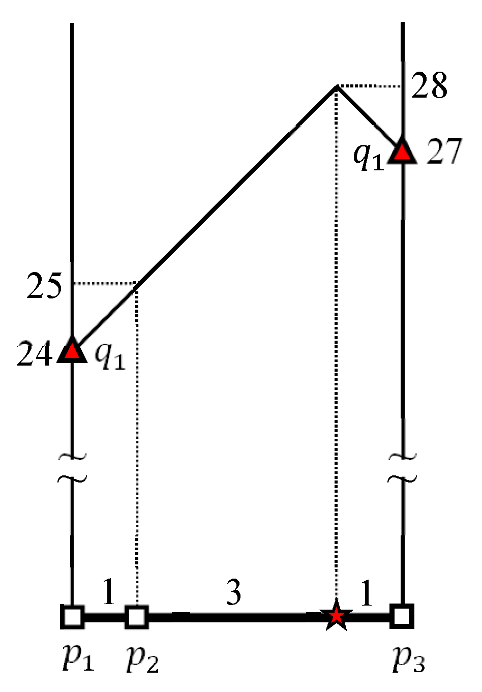
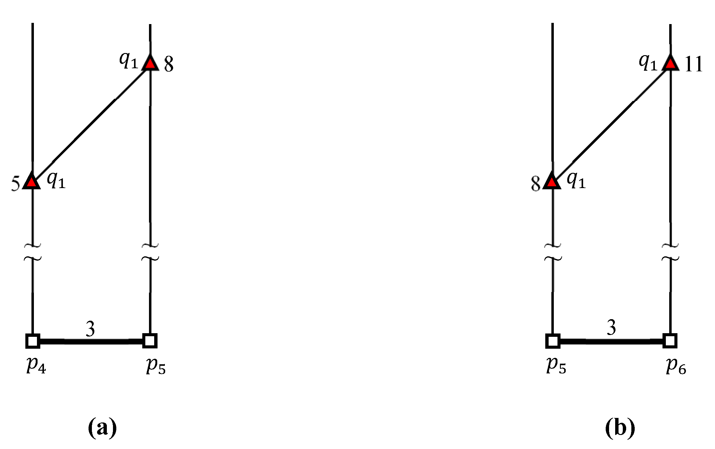
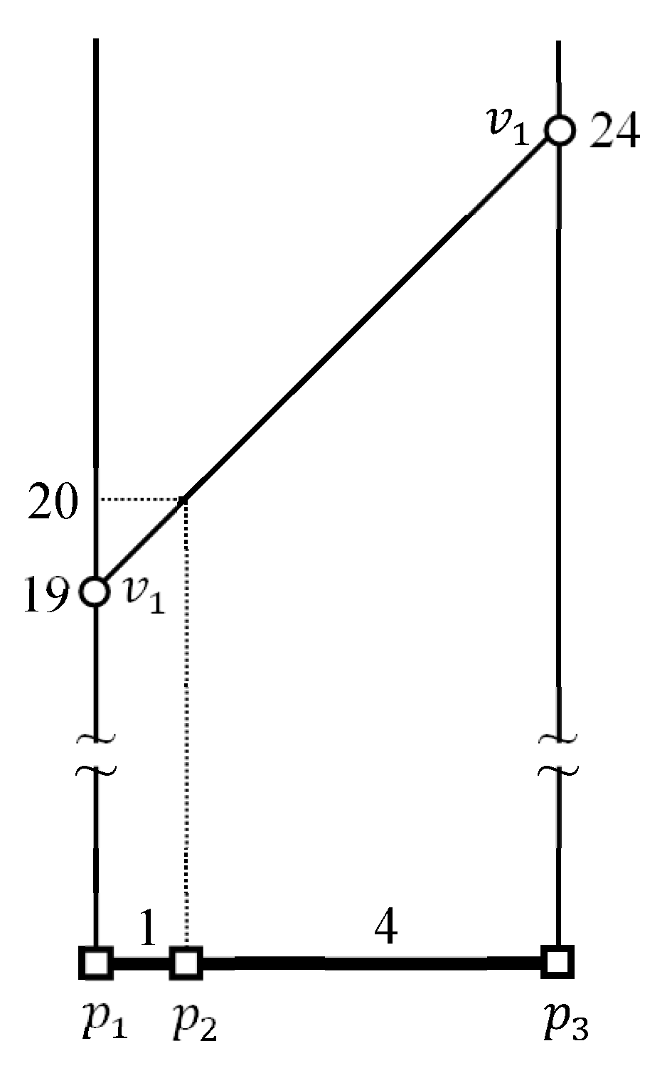
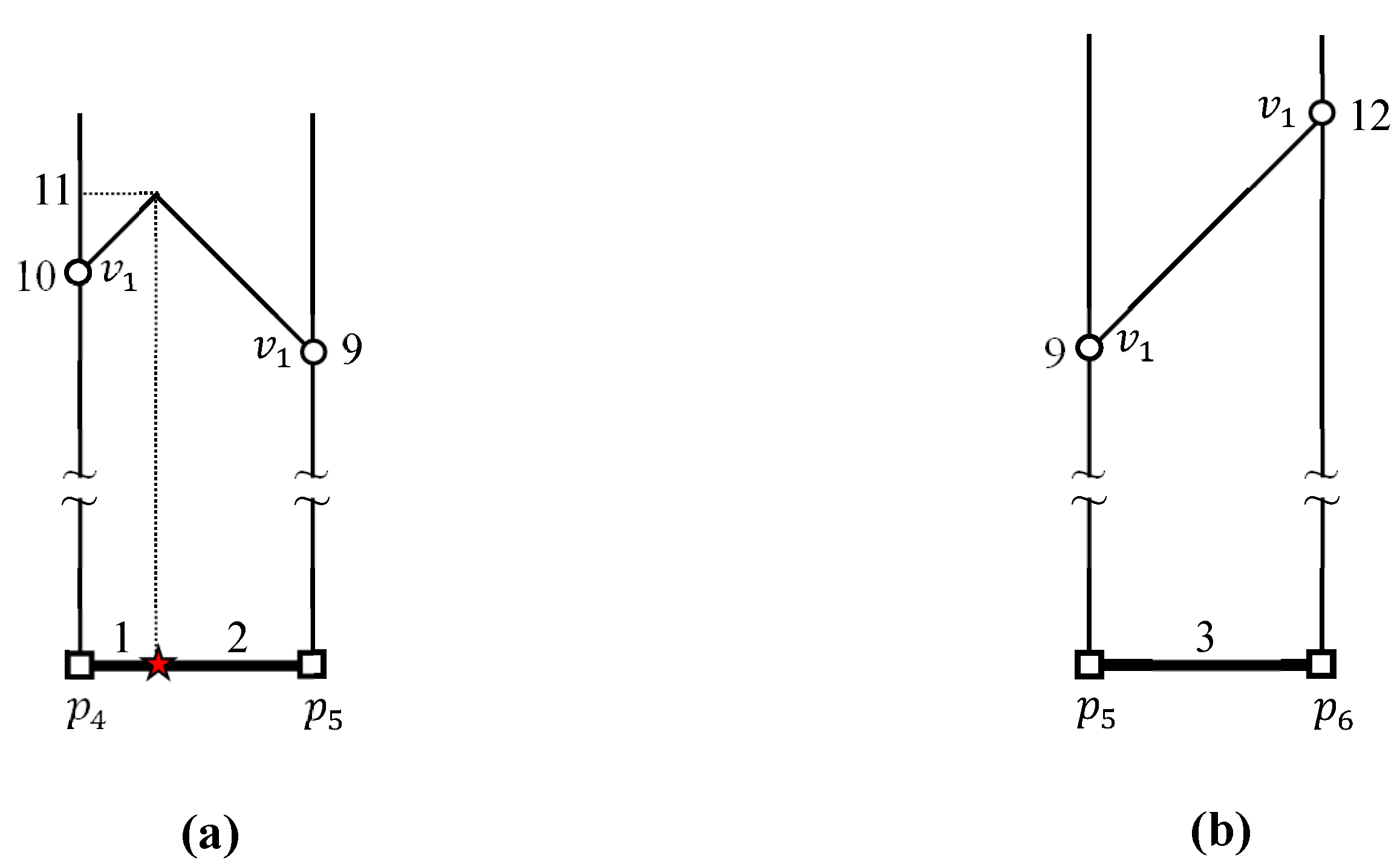
4.2. Evaluating kFN Queries at Border Points

The CNLJ algorithm evaluates kFN queries at the border points of query clusters $\overline{Q_C}$. For the example kFN join query, the CNLJ algorithm evaluates kFN queries at border points $q_1$, $v_1$, and $v_2$, rather than query points $q_1$, $q_2$, $q_3$, and $q_4$. First, the kFN query is evaluated at a border point $q_1$. The maximum and minimum distances between $q_1$ and each data cluster in $\overline{P}$ are computed, and the data clusters are sorted in descending order based on their maximum distance to $q_1$. As shown in Figure 11, the two data clusters $\left\{\overline{p_1{p}_2{p}_3}\right\}$ and $\{\overline{p_4{p}_5},\overline{p_5{p}_6}\}$ are arranged using their maximum distance to $q_1$ as follows: $\overline{P}=\{\left\{\overline{p_1{p}_2{p}_3}\right\},\{\overline{p_4{p}_5},\overline{p_5{p}_6}\}\}$. This is because $maxdist(q_1,\left\{\overline{p_1{p}_2{p}_3}\right\})=28$ and $maxdist(q_1,\{\overline{p_4{p}_5},\overline{p_5{p}_6}\})=11$, as described in Table 3. The border point $q_1$ investigates $\left\{\overline{p_1{p}_2{p}_3}\right\}$ followed by $\{\overline{p_4{p}_5},\overline{p_5{p}_6}\}$. Following an exploration of $\left\{\overline{p_1{p}_2{p}_3}\right\}$, $q_1$ selects $p_2$ and $p_3$ as the two FNs because $dist(q_1,p_1)=24$, $dist(q_1,p_2)=25$, and $dist(q_1,p_3)=27$ are computed, as shown in Figure 5. The sentinel distance for $q_1$ is $sntl\_dist=20$. This is because the maximum distance l between the border points in $\overline{Q_C}$ is $l=dist(q_1,v_1)=5$, whereas the distance from $q_1$ to its second FN $p_2$ is $dist(q_1,p_2)=25$. Thus, a set of candidate data points for query points in $\overline{Q_C}$ is $\mathrm{\Omega }\left(q_1\right)=\{p_1,p_2,p_3\}$. This is because $dist(q_1,p_1)\ge sntl\_dist$, $dist(q_1,p_2)\ge sntl\_dist$, and $dist(q_1,p_3)\ge sntl\_dist$. Clearly, $q_1$ no longer examines the other data cluster $\{\overline{p_4{p}_5},\overline{p_5{p}_6}\}$. This is because $sntl\_dist$ is larger than $maxdist(q_1,\{\overline{p_4{p}_5},\overline{p_5{p}_6}\})$ where $maxdist(q_1,\{\overline{p_4{p}_5},\overline{p_5{p}_6}\})=11$, as shown in Table 3. Finally, a set of candidate data points for query points in $\overline{Q_C}$ is $\mathrm{\Omega }\left(q_1\right)=\{p_1,p_2,p_3\}$.

At the other border points $v_1$ and $v_2$, we can similarly evaluate kFN queries. Two FNs of $v_1$ are $p_2$ and $p_3$, as illustrated in Figure 7 and Figure 8. Thus, a set of candidate data points at $v_1$ is $\mathrm{\Omega }\left(v_1\right)=\{p_1,p_2,p_3\}$ because the sentinel distance for $v_1$ is $sntl\_dist\left(v_1\right)=15$. Similarly, two FNs of $v_2$ are $p_1$ and $p_2$, as illustrated in Figure 9 and Figure 10. Thus, a set of candidate data points at $v_2$ is $\mathrm{\Omega }\left(v_2\right)=\{p_1,p_2,p_3\}$ because the sentinel distance for $v_2$ is $sntl\_dist\left(v_2\right)=18$.

Table 5. Results of kFN queries at $q_1$, $v_1$, and $v_2$ and their sentinel distances.

${\mathit{b}}_{\mathit{q}}$	$\mathit{dist}({\mathit{b}}_{\mathit{q}},\mathit{p})$	$\mathit{sntl}\_\mathit{dist}\left({\mathit{b}}_{\mathit{q}}\right)$	$\mathbf{\Omega }\left({\mathit{b}}_{\mathit{q}}\right)$
$q_1$	$dist(q_1,p_1)=24$	$sntl\_dist\left(q_1\right)=20$	$\mathrm{\Omega }\left(q_1\right)=\{p_1,p_2,p_3\}$
	$dist(q_1,p_2)=25$
	$dist(q_1,p_3)=27$
$v_1$	$dist(v_1,p_1)=19$	$sntl\_dist\left(v_1\right)=15$	$\mathrm{\Omega }\left(v_1\right)=\{p_1,p_2,p_3\}$
	$dist(v_1,p_2)=20$
	$dist(v_1,p_3)=24$
$v_2$	$dist(v_2,p_1)=23$	$sntl\_dist\left(v_2\right)=18$	$\mathrm{\Omega }\left(v_2\right)=\{p_1,p_2,p_3\}$
	$dist(v_2,p_2)=24$
	$dist(v_2,p_3)=23$

summarizes sets of candidate data points for border points $q_1$, $v_1$, and $v_2$ and their sentinel distance.

4.3. Evaluating an Example kFN Join Query

The CNLJ algorithm retrieves k FNs for each query point in $\overline{Q_C}$ among the candidate data points in $\mathrm{\Omega }\left(B\left(\overline{Q_C}\right)\right)$. This example kFN join query requires two FNs for each query point, i.e., $k=2$, and the set of candidate data points is $\mathrm{\Omega }\left(B\left(\overline{Q_C}\right)\right)=\{p_1,p_2,p_3\}$. Each of $q_1$, $q_2$, $q_3$, and $q_4$ retrieves its two FNs among candidate data points $p_1$, $p_2$, and $p_3$. Two FNs of $q_1$ are first determined, two FNs of $q_2$ are next determined, and so on. Let us find two FNs for $q_1$ among the candidate data points $p_1$, $p_2$, and $p_3$. The distances from $q_1$ to $p_1$, $p_2$, and $p_3$ should be computed using the fact that the shortest path from $q_1$ to a candidate data point should pass through a border point $b_q$. As a result, the length of the shortest path from $q_1$ to $p_1$ is equal to $dist(q_1,p_1)$ $=min\{dist(q_1,b_q)+dist(b_q,p_1)\left|\phantom{dist(q_1,b_q)+dist(b_q,p_1)b_q\in \{q_1,v_1,v_2\}}\right.b_q\in \{q_1,v_1,v_2\}\}$ $=min\{dist(q_1,q_1)+dist(q_1,p_1),$$dist(q_1,v_1)+dist(v_1,p_1),$$dist(q_1,v_2)+dist(v_2,p_1)\}$ $=min\{24,24,27\}=24$. The distance from $q_1$ to $p_2$ evaluates to $dist(q_1,p_2)=$ $min\{dist(q_1,b_q)+dist(b_q,p_2)\left|\phantom{dist(q_1,b_q)+dist(b_q,p_2)b_q\in \{q_1,v_1,v_2\}}\right.b_q\in \{q_1,v_1,v_2\}\}=25$. The distance from $q_1$ to $p_3$ evaluates to $dist(q_1,p_3)=min\{dist(q_1,b_q)+dist(b_q,p_3)\left|\phantom{dist(q_1,b_q)+dist(b_q,p_3)b_q\in \{q_1,v_1,v_2\}}\right.b_q\in \{q_1,v_1,v_2\}\}=27$. Thus, $p_2$ and $p_3$ are two FNs for $q_1$ whose result set is $\mathrm{\Omega }\left(q_1\right)=\{p_2,p_3\}$. Next, two FNs for $q_2$ are retrieved among candidate data points $p_1$, $p_2$, and $p_3$. For this, the distances from $q_2$ to $p_1$, $p_2$, and $p_3$ should be computed. As shown in

Table 6. Retrieval of two FNs for query points among candidate data points.

q	$\mathit{dist}(\mathit{q},\mathit{p})$	$\mathbf{\Omega }\left(\mathit{q}\right)$
$q_1$	$dist(q_1,p_1)=24$	$\mathrm{\Omega }\left(q_1\right)=\{p_2,p_3\}$
	$dist(q_1,p_2)=25$
	$dist(q_1,p_3)=27$
$q_2$	$dist(q_2,p_1)=25$	$\mathrm{\Omega }\left(q_2\right)=\{p_1,p_2\}$ or
	$dist(q_2,p_2)=26$	$\mathrm{\Omega }\left(q_2\right)=\{p_2,p_3\}$
	$dist(q_2,p_3)=25$
$q_3$	$dist(q_3,p_1)=21$	$\mathrm{\Omega }\left(q_3\right)=\{p_2,p_3\}$
	$dist(q_3,p_2)=22$
	$dist(q_3,p_3)=25$
$q_4$	$dist(q_4,p_1)=21$	$\mathrm{\Omega }\left(q_4\right)=\{p_2,p_3\}$
	$dist(q_4,p_2)=22$
	$dist(q_4,p_3)=26$

, the distances from $q_2$ to $p_1$, $p_2$, and $p_3$ evaluate to $dist(q_2,p_1)=25$, $dist(q_2,p_2)=26$, and $dist(q_2,p_3)=25$, respectively. Thus, $p_1$ and $p_2$ are two FNs for $q_2$, whose result set is $\mathrm{\Omega }\left(q_2\right)=\{p_1,p_2\}$. Similarly, two FNs for $q_3$ and $q_4$ can be retrieved among candidate data points $p_1$, $p_2$, and $p_3$. Table 6 computes the distance from a query point q to a candidate data point p and retrieves two FNs for q among candidate data points where $q\in \{q_1,q_2,q_3,q_4\}$ and $p\in \{p_1,p_2,p_3\}$. Finally, the kFN join result is the union set of the kFN query results for query points in Q as follows: $\mathrm{\Omega }\left(Q\right)=\mathrm{\Omega }\left(q_1\right)\cup \mathrm{\Omega }\left(q_2\right)\cup \mathrm{\Omega }\left(q_3\right)\cup \mathrm{\Omega }\left(q_4\right)=\{〈q_1,\{p_2,p_3\}〉,〈q_2,\{p_1,p_2\}〉,〈q_3,\{p_2,p_3\}〉,〈q_4,\{p_2,p_3\}〉\}$.

5. Performance Evaluation

The CNLJ algorithm and its competitors are compared empirically in this section under a variety of conditions. Section 5.1 describes the experimental conditions, and Section 5.2 reports the results of the experiment.

5.1. Experimental Settings

Table 7. Real-world roadmaps [40].

Name	Description	Vertices	Edges	Vertex Sequences
NA	Highways in North America (NA)	175,813	179,179	12,416
SJ	City streets in San Joaquin (SJ), California	18,263	23,874	20,040

describes two real-world roadmaps [40] that were used in the experiments. These real-world roadmaps have different sizes and are part of the United States’ road network. For convenience, the data universe was normalized to a unit square of the plane. The query and data points were generated to mimic the highly skewed distributions of POIs in the real world. Firstly, the centroids $c_1,c_2,\cdots ,c_m$ were randomly chosen inside the data universe, where m indicates the total number of centroids and varies between 1 and 10. The query and data points around each centroid displayed a normal distribution, with the mean indicating the centroid and the standard deviation set to ${\sigma =10}^{-2}$.

Table 8. Experimental parameter settings.

Parameter	Range
Number of query points ($\left|Q\right|$)	1, 2, 3, 4, 5, 7, 10 ($\times {10}^3$)
Number of data points ($\left|P\right|$)	1, 2, 3, 4, 5, 7, 10 ($\times {10}^3$)
Number of FNs required (k)	1, 2, 4, 8, 16
Distribution of query and data points	Centroid distribution
Number of centroids for query points in Q ($|C_Q|$)	1, 3, 5, 7, 10
Number of centroids for data points in P ($|C_P|$)	1, 3, 5, 7, 10
The standard deviation for normal distribution ($\sigma$)	${\mathbf{10}}^{-\mathbf{2}}$
Roadmap	NA, SJ

shows the experimental parameters settings. We varied a single parameter within the range in each experiment while maintaining the other parameters at the bold default values.

The baseline algorithm, which is a nonclustering join algorithm for sequentially computing the k FNs of each query point in Q, was used as a benchmark for evaluating the CNLJ algorithm. We implemented and evaluated two versions of our proposed solution, i.e., CNLJ${}_{\mathrm{NV}}$ and CNLJ${}_{\mathrm{OPT}}$. The naive version called CNLJ${}_{\mathrm{NV}}$ of the CNLJ algorithm groups query points into query segments, as illustrated in Figure 3a. Thus, CNLJ${}_{\mathrm{NV}}$ evaluates at most two kFN queries for a query segment. The optimized version called CNLJ${}_{\mathrm{OPT}}$ of the CNLJ algorithm groups query points into query clusters using the two-step clustering method, as illustrated in Figure 3b. Note that the source codes for empirical evaluation of this study can be accessed via the GitHub site at https://github.com/Hyung-Ju-Cho/ (accessed on 8 February 2021). In the Microsoft Visual Studio 2019 development environment, all join algorithms were implemented in C++. All of the algorithms’ common subroutines were reused for similar tasks. Experiments were conducted on a desktop computer running the Windows 10 operating system with 32 GB RAM and an 8-core processor (i9-9900) at 3.1 GHz. As in several existing studies [36,41] for online map services, this empirical study assumes that all of the algorithms’ indexing structures remain in the main memory to evaluate kFN join queries quickly. The average time required to answer kFN join queries was calculated through repeated experiments using kFN join queries. Finally, we computed the network distance between two points quickly using the TNR method [42]. This is because the TNR method is easy to implement and demonstrates performance comparable to the other shortest distance algorithms [38,41,43,44,45].

5.2. Experimental Results

The proposed CNLJ${}_{\mathrm{OPT}}$, CNLJ${}_{\mathrm{NV}}$, and baseline algorithms in the NA roadmap are compared in Figure 12. Each chart shows the kFN join query processing time and the number of kFN queries required to evaluate the kFN join query. The numbers of kFN queries required by the CNLJ${}_{\mathrm{OPT}}$, CNLJ${}_{\mathrm{NV}}$, and baseline algorithms to answer the kFN join query are shown in parentheses in Figure 12, Figure 13 and Figure 14. Note that the CNLJ${}_{\mathrm{OPT}}$ algorithm evaluates kFN queries at border points of query clusters, the CNLJ${}_{\mathrm{NV}}$ algorithm evaluates kFN queries at end points of query segments, and the baseline algorithm evaluates kFN queries at query points. As a result, the baseline algorithm evaluates the same number of kFN queries as the number $\left|Q\right|$ of query points in Q. Figure 12a shows the query processing times of the CNLJ${}_{\mathrm{OPT}}$, CNLJ${}_{\mathrm{NV}}$, and baseline algorithms when the number of the query points changes between 1000 and 5000, i.e., $1000\le \left|Q\right|\le 5000$. In all cases in $\left|Q\right|$, the CNLJ${}_{\mathrm{OPT}}$ algorithm is faster than the CNLJ${}_{\mathrm{NV}}$ and baseline algorithms. When $\left|Q\right|=5000$, the CNLJ${}_{\mathrm{OPT}}$, CNLJ${}_{\mathrm{NV}}$, and baseline algorithms evaluate 281, 471, and 5000 kFN queries, respectively, and thus the CNLJ${}_{\mathrm{OPT}}$ algorithm is 1.2 and 36.7 times faster than the CNLJ${}_{\mathrm{NV}}$ and baseline algorithms, respectively. Figure 12b shows the query processing times when the number of data points changes from 1000 to 5000, i.e., $1000\le \left|P\right|\le 5000$. Regardless of the $\left|P\right|$ value, the CNLJ${}_{\mathrm{OPT}}$, CNLJ${}_{\mathrm{NV}}$, and baseline algorithms evaluate 58, 96, and 1000 kFN queries, respectively. Thus, when $\left|P\right|=3000$, the CNLJ${}_{\mathrm{OPT}}$ algorithm outperforms the CNLJ${}_{\mathrm{NV}}$ and baseline algorithms by 1.2 and 15.6 times, respectively. Figure 12c shows the query processing times when the number of FNs required changes between 1 and 16, i.e., $1\le k\le 16$. For all cases in k, the CNLJ${}_{\mathrm{OPT}}$ algorithm outperforms the CNLJ${}_{\mathrm{NV}}$ and baseline algorithms by 1.2 and 13.4 times, respectively. The CNLJ${}_{\mathrm{OPT}}$, CNLJ${}_{\mathrm{NV}}$, and baseline algorithms’ query processing times are not affected by the k value. This is because the kFN query evaluation computes the distances from a query point to data clusters, regardless of the k value, and then sorts the data clusters using the distances to the query point. Figure 12d shows the query processing times when the number of centroids for query points in Q changes between 1 and 10, i.e., $1\le |C_Q|\le 10$. As the $|C_Q|$ value increases, the difference between the query processing times of all algorithms decreases. The CNLJ${}_{\mathrm{OPT}}$ algorithm is 13.3, 1.3, 1.6, 1.7, and 1.1 times faster than the baseline algorithm when $|C_Q|=$ 1, 3, 5, 7, and 10, respectively. The reason is that as the $|C_Q|$ value increases, the query points are widely dispersed and the number of query clusters increases, slowing down the CNLJ${}_{\mathrm{OPT}}$ algorithm’s query processing time. Figure 12e shows the query processing times when the number of centroids for data points in P changes between 1 and 10, i.e., $1\le |C_P|\le 10$. The kFN query processing time increases with the $|C_P|$ value. This is because as the $|C_P|$ value increases, the data points are widely dispersed and the number of data clusters to be examined by the kFN queries also increases. To summarize, the CNLJ${}_{\mathrm{OPT}}$ algorithm outperforms the CNLJ${}_{\mathrm{NV}}$ and baseline algorithms in all the cases. This confirms that the CNLJ${}_{\mathrm{OPT}}$ algorithm benefits from clustering of nearby query points and quickly retrieving candidate data points at once for those query points.

In the SJ roadmap, Figure 13 compares the performance of the CNLJ${}_{\mathrm{OPT}}$, CNLJ${}_{\mathrm{NV}}$, and baseline algorithms. Note that the experimental results using the SJ roadmap exhibit similar performance patterns to those using the NA roadmap. Figure 13a shows the query processing times when $1000\le \left|Q\right|\le 5000$. The CNLJ${}_{\mathrm{OPT}}$ algorithm is 1.2 and 6.0 times faster than the CNLJ${}_{NV}$ and baseline algorithms when $\left|Q\right|=5000$, respectively. Figure 13b shows the query processing times when $1000\le \left|P\right|\le 5000$. The CNLJ${}_{\mathrm{OPT}}$ algorithm is 1.2 and 4.5 times faster than the CNLJ${}_{\mathrm{NV}}$ and baseline algorithms when $\left|P\right|=4000$, respectively. The $\left|P\right|$ value increases the query processing times of all algorithms. Figure 13c shows the query processing times when $1\le k\le 16$. The CNLJ${}_{\mathrm{OPT}}$ algorithm is 1.2 and 3.5 times faster than the CNLJ${}_{\mathrm{NV}}$ and baseline algorithms, respectively. The query processing times are nearly constant regardless of the k value. Figure 13d shows the query processing times when $1\le |C_Q|\le 10$. The CNLJ${}_{\mathrm{OPT}}$ algorithm is 3.5, 2.4, 1.8, 1.4, and 1.4 times faster than the baseline algorithm when $|C_Q|$ = 1, 3, 5, 7, and 10, respectively. The distribution of query points has an impact on the query processing time of the CNLJ${}_{\mathrm{OPT}}$ algorithm, as shown by this result. The query processing time of the CNLJ${}_{\mathrm{OPT}}$ algorithm increases with the number of query clusters because the query points are widely dispersed. Figure 13e shows the query processing times when $1\le |C_P|\le 10$. The CNLJ${}_{\mathrm{OPT}}$ algorithm is 2.8, 4.0, 3.5, 2.9, and 3.0 times faster than the baseline algorithm when $\left|C_P\right|$ = 1, 3, 5, 7, and 10, respectively.

Figure 14 compares the performance of the CNLJ${}_{\mathrm{OPT}}$, CNLJ${}_{\mathrm{NV}}$, and baseline algorithms while the numbers of query and data points change between 1000 and 10,000, i.e., $1000\le \left|Q\right|\le 10,000$ and $1000\le \left|P\right|\le 10,000$, to verify the scalability of the CNLJ${}_{\mathrm{OPT}}$ algorithm. As shown in Figure 14a,c, the CNLJ${}_{\mathrm{OPT}}$ algorithm runs faster than the CNLJ${}_{\mathrm{NV}}$ and baseline algorithms for all cases in $\left|Q\right|$. The performance difference between them typically increases with $\left|Q\right|$. Specifically, when $\left|Q\right|=10,000$, the CNLJ${}_{\mathrm{OPT}}$ algorithm runs 36.6 and 5.3 times faster than the baseline algorithm for NA and SJ roadmaps, respectively. As shown in Figure 14b,d, the CNLJ${}_{\mathrm{OPT}}$ algorithm runs faster than the CNLJ${}_{\mathrm{NV}}$ and baseline algorithms for all cases in $\left|P\right|$. Specifically, when $\left|P\right|=10,000$, the CNLJ${}_{\mathrm{OPT}}$ algorithm runs 6.4 and 3.0 times faster than the baseline algorithm for NA and SJ roadmaps, respectively. The experimental results confirm that the CNLJ${}_{\mathrm{OPT}}$ algorithm scales better with both $\left|Q\right|$ and $\left|P\right|$ than the CNLJ${}_{\mathrm{NV}}$ and baseline algorithms.

6. Discussion and Conclusions

The kFN join query retrieves a pair of each query point in Q with its k FNs in P, given a positive integer k, a set of query points Q, and a set of data points P. The kFN join query has various real-life applications including recommender systems and computational geometry [6,7,8,9,10,11,12,13,14]. In particular, efficient processing of kFN join queries can aid in selecting a facility’s location that is farthest away from unpleasant facilities such as garbage incinerators, crematoriums, and chemical plants. A cluster nested loop join (CNLJ) algorithm was constructed in this study to efficiently answer kFN join queries for spatial networks. To the best of our knowledge, this is the first attempt to study kFN join queries in spatial networks. The CNLJ algorithm converts query points (data points) into query clusters (data clusters). It then retrieves candidate data points for clustered query points all at once, eliminating the need to search for candidate data points for each query point separately. Using real-life roadmaps in various conditions, the query processing times of the CNLJ and conventional join algorithms were empirically compared. The experimental results demonstrated that the CNLJ algorithm runs up to 50.8 times faster than the conventional join algorithms and that the CNLJ algorithm also better scales with the numbers of both data and query points than the conventional join algorithms. Unfortunately, the CNLJ algorithm shows similar performance to the conventional join algorithms, particularly when query points are uniformly located in the region. We intend to apply the proposed solution to various fields in the future. When the dataset does not fit in the main memory, we will first create index structures on the external memory. Second, we will conduct an empirical study to simulate real-life scenarios using real datasets. Third, we will improve the CNLJ algorithm for the efficient processing of kFN joins over query points that are uniformly scattered in the region.

References

1. Said, A.; Kille, B.; Jain, B.J.; Albayrak, S. Increasing diversity through furthest neighbor-based recommendation. In Proceedings of the International Workshop on Diversity in Document Retrieval, Seattle, WA, USA, 12 February 2012; pp. 1–4. [Google Scholar]
2. Said, A.; Fields, B.; Jain, B.J.; Albayrak, S. User-centric evaluation of a k-furthest neighbor collaborative filtering recommender algorithm. In Proceedings of the International Conference on Computer Supported Cooperative Work and Social Computing, San Antonio, TX, USA, 23–27 February 2013; pp. 1399–1408. [Google Scholar]
3. Veenman, C.J.; Reinders, M.J.T.; Backer, E. A maximum variance cluster algorithm. IEEE Trans. Pattern Anal. Mach. Intell. 2002, 24, 1273–1280. [Google Scholar] [CrossRef] [Green Version]
4. Defays, D. An efficient algorithm for a complete link method. Comput. J. 1977, 20, 364–366. [Google Scholar] [CrossRef] [Green Version]
5. Vasiloglou, N.; Gray, A.G.; Anderson, D.V. Scalable semidefinite manifold learning. In Proceedings of the IEEE Workshop on Machine Learning for Signal Processing, Cancun, Mexico, 16–19 October 2008; pp. 368–373. [Google Scholar]
6. Curtin, R.R.; Echauz, J.; Gardner, A.B. Exploiting the structure of furthest neighbor search for fast approximate results. Inf. Syst. 2019, 80, 124–135. [Google Scholar] [CrossRef]
7. Gao, Y.; Shou, L.; Chen, K.; Chen, G. Aggregate farthest-neighbor queries over spatial data. In Proceedings of the International Conference on Database Systems for Advanced Applications, Hong Kong, China, 22–25 April 2011; pp. 149–163. [Google Scholar]
8. Liu, J.; Chen, H.; Furuse, K.; Kitagawa, H. An efficient algorithm for arbitrary reverse furthest neighbor queries. In Proceedings of the Asia-Pacific Web Conference on Web Technologies and Applications, Kunming, China, 11–13 April 2012; pp. 60–72. [Google Scholar]
9. Liu, W.; Yuan, Y. New ideas for FN/RFN queries based nearest Voronoi diagram. In Proceedings of the International Conference on Bio-Inspired Computing: Theories and Applications, Huangshan, China, 12–14 July 2013; pp. 917–927. [Google Scholar]
10. Tran, Q.T.; Taniar, D.; Safar, M. Reverse k nearest neighbor and reverse farthest neighbor search on spatial networks. Trans. Large-Scale Data-Knowl.-Cent. Syst. 2009, 1, 353–372. [Google Scholar]
11. Wang, H.; Zheng, K.; Su, H.; Wang, J.; Sadiq, S.W.; Zhou, X. Efficient aggregate farthest neighbour query processing on road networks. In Proceedings of the Australasian Database Conference on Databases Theory and Applications, Brisbane, Australia, 14–16 July 2014; pp. 13–25. [Google Scholar]
12. Xiao, Y.; Liu, B.; Hao, Z.; Cao, L. A k-farthest-neighbor-based approach for support vector data description. Appl. Intell. 2014, 41, 196–211. [Google Scholar] [CrossRef]
13. Xu, X.-J.; Bao, J.-S.; Yao, B.; Zhou, J.-Y.; Tang, F.-L.; Guo, M.-Y.; Xu, J.-Q. Reverse furthest neighbors query in road networks. J. Comput. Sci. Technol. 2017, 32, 155–167. [Google Scholar] [CrossRef]
14. Yao, B.; Li, F.; Kumar, P. Reverse furthest neighbors in spatial databases. In Proceedings of the International Conference on Data Engineering, Shanghai, China, 29 March–2 April 2009; pp. 664–675. [Google Scholar]
15. Dutta, B.; Karmakar, A.; Roy, S. Optimal facility location problem on polyhedral terrains using descending paths. Theor. Comput. Sci. 2020, 847, 68–75. [Google Scholar] [CrossRef]
16. Gao, X.; Park, C.; Chen, X.; Xie, E.; Huang, G.; Zhang, D. Globally optimal facility locations for continuous-space facility location problems. Appl. Sci. 2021, 11, 7321. [Google Scholar] [CrossRef]
17. Liu, W.; Wang, H.; Zhang, Y.; Qin, L.; Zhang, W. I/O efficient algorithm for c-approximate furthest neighbor search in high-dimensional space. In Proceedings of the International Conference on Database Systems for Advanced Applications, Jeju, Korea, 24–27 September 2020; pp. 221–236. [Google Scholar]
18. Huang, Q.; Feng, J.; Fang, Q.; Ng, W. Two efficient hashing schemes for high-dimensional furthest neighbor search. IEEE Trans. Knowl. Data Eng. 2017, 29, 2772–2785. [Google Scholar] [CrossRef]
19. Liu, Y.; Gong, X.; Kong, D.; Hao, T.; Yan, X. A Voronoi-based group reverse k farthest neighbor query method in the obstacle space. IEEE Access 2020, 8, 50659–50673. [Google Scholar] [CrossRef]
20. Pagh, R.; Silvestri, F.; Sivertsen, J.; Skala, M. Approximate furthest neighbor in high dimensions. In Proceedings of the International Conference on Similarity Search and Applications, Glasgow, UK, 12–14 October 2015; pp. 3–14. [Google Scholar]
21. Korn, F.; Muthukrishnan, S. Influence sets based on reverse nearest neighbor queries. In Proceedings of the International Conference on Management of Data, Dallas, TX, USA, 16–18 May 2000; pp. 201–212. [Google Scholar]
22. Wang, S.; Cheema, M.A.; Lin, X.; Zhang, Y.; Liu, D. Efficiently computing reverse k furthest neighbors. In Proceedings of the International Conference on Data Engineering, Helsinki, Finland, 16–20 May 2016; pp. 1110–1121. [Google Scholar]
23. Beckmann, N.; Kriegel, H.-P.; Schneider, R.; Seeger, B. The R*-tree: An efficient and robust access method for points and rectangles. In Proceedings of the International Conference on Management of Data, Atlantic City, NJ, USA, 23–25 May 1990; pp. 322–331. [Google Scholar]
24. Guttman, A. R-trees: A dynamic index structure for spatial searching. In Proceedings of the International Conference on Management of Data, Boston, MA, USA, 18–21 June 1984; pp. 47–57. [Google Scholar]
25. Huang, Q.; Feng, J.; Fang, Q. Reverse query-aware locality-sensitive hashing for high-dimensional furthest neighbor search. In Proceedings of the International Conference on Data Engineering, San Diego, CA, USA, 19–22 April 2017; pp. 167–170. [Google Scholar]
26. Lu, H.; Yiu, M.L. On computing farthest dominated locations. IEEE Trans. Knowl. Data Eng. 2011, 23, 928–941. [Google Scholar] [CrossRef]
27. Cho, H.-J. Efficient shared execution processing of k-nearest neighbor joins in road networks. Mob. Inf. Syst. 2018, 2018, 55–66. [Google Scholar] [CrossRef] [Green Version]
28. He, D.; Wang, S.; Zhou, X.; Cheng, R. GLAD: A grid and labeling framework with scheduling for conflict-aware knn Queries. IEEE Trans. Knowl. Data Eng. 2021, 33, 1554–1566. [Google Scholar] [CrossRef]
29. Yang, R.; Niu, B. Continuous k nearest neighbor queries over large-scale spatial-textual data streams. ISPRS Int. J. Geo-Inf. 2020, 9, 694. [Google Scholar] [CrossRef]
30. Cho, H.-J.; Attique, M. Group processing of multiple k-farthest neighbor queries in road networks. IEEE Access 2020, 8, 110959–110973. [Google Scholar] [CrossRef]
31. Reza, R.M.; Ali, M.E.; Hashem, T. Group processing of simultaneous shortest path queries in road networks. In Proceedings of the International Conference on Mobile Data Management, Pittsburgh, PA, USA, 15–18 June 2015; pp. 128–133. [Google Scholar]
32. Zhang, M.; Li, L.; Hua, W.; Zhou, X. Efficient batch processing of shortest path queries in road networks. In Proceedings of the International Conference on Mobile Data Management, Hong Kong, China, 10–13 June 2019; pp. 100–105. [Google Scholar]
33. Zhang, M.; Li, L.; Hua, W.; Zhou, X. Batch processing of shortest path queries in road networks. In Proceedings of the Australasian Database Conference on Databases Theory and Applications, Sydney, Australia, 29 January–1 February 2019; pp. 3–16. [Google Scholar]
34. Reza, R.M.; Ali, M.E.; Cheema, M.A. The optimal route and stops for a group of users in a road network. In Proceedings of the International Conference on Advances in Geographic Information Systems, Redondo Beach, CA, USA, 7–10 November 2017; pp. 1–10. [Google Scholar]
35. Kim, T.; Cho, H.-J.; Hong, H.J.; Nam, H.; Cho, H.; Do, G.Y.; Jeon, P. Efficient processing of k-farthest neighbor queries for road networks. J. Korea Soc. Comput. Inf. 2019, 24, 79–89. [Google Scholar]
36. Abeywickrama, T.; Cheema, M.A.; Taniar, D. k-nearest neighbors on road networks: A journey in experimentation and in-memory implementation. In Proceedings of the International Conference on Very Large Data Bases, New Delhi, India, 5–9 September 2016; pp. 492–503. [Google Scholar]
37. Lee, K.C.K.; Lee, W.-C.; Zheng, B.; Tian, Y. ROAD: A new spatial object search framework for road networks. IEEE Trans. Knowl. Data Eng. 2012, 24, 547–560. [Google Scholar] [CrossRef]
38. Zhong, R.; Li, G.; Tan, K.-L.; Zhou, L.; Gong, Z. G-tree: An efficient and scalable index for spatial search on road networks. IEEE Trans. Knowl. Data Eng. 2015, 27, 2175–2189. [Google Scholar] [CrossRef]
39. Cormen, T.H.; Leiserson, C.E.; Rivest, R.L.; Stein, C. Introduction to Algorithms, 3rd ed.; MIT Press and McGraw-Hill: Cambridge, MA, USA, 2009; pp. 643–683. [Google Scholar]
40. Real Datasets for Spatial Databases. Available online: https://www.cs.utah.edu/~lifeifei/SpatialDataset.htm (accessed on 4 October 2021).
41. Wu, L.; Xiao, X.; Deng, D.; Cong, G.; Zhu, A.D.; Zhou, S. Shortest path and distance queries on road networks: An experimental evaluation. In Proceedings of the International Conference on Very Large Data Bases, Istanbul, Turkey, 27–31 August 2012; pp. 406–417. [Google Scholar]
42. Bast, H.; Funke, S.; Matijevic, D. Ultrafast shortest-path queries via transit nodes. In Proceedings of the International Workshop on Shortest Path Problem, Piscataway, NJ, USA, 13–14 November 2006; pp. 175–192. [Google Scholar]
43. Geisberger, R.; Sanders, P.; Schultes, D.; Delling, D. Contraction hierarchies: Faster and simpler hierarchical routing in road networks. In Proceedings of the International Workshop on Experimental Algorithms, Cape Cod, MA, USA, 30 May–2 June 2008; pp. 319–333. [Google Scholar]
44. Li, Z.; Chen, L.; Wang, Y. G*-tree: An efficient spatial index on road networks. In Proceedings of the International Conference on Data Engineering, Macao, China, 8–11 April 2019; pp. 268–279. [Google Scholar]
45. Samet, H.; Sankaranarayanan, J.; Alborzi, H. Scalable network distance browsing in spatial databases. In Proceedings of the International Conference on Management of Data, Vancouver, BC, Canada, 9–12 June 2008; pp. 43–54. [Google Scholar]
Figure 1. Example of kFN join Q k F N P , where Q = { q 1 , q 2 , q 3 } and P = { p 1 , p 2 , p 3 , p 4 } .
Ijgi 11 00123 g001
Figure 2. Example of kFN join Q P in a spatial network.
Ijgi 11 00123 g002
Figure 3. Two-step clustering method to group nearby query points into query clusters: (a) converting query points into query segments; (b) converting query segments into query clusters.
Ijgi 11 00123 g003
Figure 4. Two-step clustering method to group nearby data points into a data cluster: (a) converting data points into data segments; (b) converting data segments into data clusters.
Ijgi 11 00123 g004
Figure 5. m a x d i s t ( q 1 , { p 1 p 2 p 3 ¯ } ) = 28 and m i n d i s t ( q 1 , { p 1 p 2 p 3 ¯ } ) = 24 .
Ijgi 11 00123 g005
Figure 6. m a x d i s t ( q 1 , { p 4 p 5 ¯ , p 5 p 6 ¯ } ) = 11 and m i n d i s t ( q 1 , { p 4 p 5 ¯ , p 5 p 6 ¯ } ) = 5 : (a) m a x d i s t ( q 1 , p 4 p 5 ¯ ) = 8 and m i n d i s t ( q 1 , p 4 p 5 ¯ ) = 5 ; (b) m a x d i s t ( q 1 , p 5 p 6 ¯ ) = 11 and m i n d i s t ( q 1 , p 5 p 6 ¯ ) = 8 .
Ijgi 11 00123 g006
Figure 7. m a x d i s t ( v 1 , { p 1 p 2 p 3 ¯ } ) = 24 and m i n d i s t ( v 1 , { p 1 p 2 p 3 ¯ } ) = 19 .
Ijgi 11 00123 g007
Figure 8. m a x d i s t ( v 1 , { p 4 p 5 ¯ , p 5 p 6 ¯ } ) = 12 and m i n d i s t ( v 1 , { p 4 p 5 ¯ , p 5 p 6 ¯ } ) = 9 : (a) m a x d i s t ( v 1 , p 4 p 5 ¯ ) = 11 and m i n d i s t ( v 1 , p 4 p 5 ¯ ) = 9 ; (b) m a x d i s t ( v 1 , p 5 p 6 ¯ ) = 12 and m i n d i s t ( v 1 , p 5 p 6 ¯ ) = 9 .
Ijgi 11 00123 g008
Figure 9. m a x d i s t ( v 2 , { p 1 p 2 p 3 ¯ } ) = 25.5 and m i n d i s t ( v 2 , { p 1 p 2 p 3 ¯ } ) = 23 .
Ijgi 11 00123 g009
Figure 10. m a x d i s t ( v 2 , { p 4 p 5 ¯ , p 5 p 6 ¯ } ) = 8 and m i n d i s t ( v 2 , { p 4 p 5 ¯ , p 5 p 6 ¯ } ) = 5 : (a) m a x d i s t ( v 2 , p 4 p 5 ¯ ) = 8 and m i n d i s t ( v 2 , p 4 p 5 ¯ ) = 5 ; (b) m a x d i s t ( v 2 , p 5 p 6 ¯ ) = 8 and m i n d i s t ( v 2 , p 5 p 6 ¯ ) = 5 .
Ijgi 11 00123 g010
Figure 11. Arranging data clusters in decreasing order of their maximum distance to q 1 .
Ijgi 11 00123 g011
Figure 12. Comparison of kFN join query processing times for the NA roadmap: (a) 10 3 Q 5 × 10 3 ; (b) 10 3 P 5 × 10 3 ; (c) 1 k 16 ; (d) 1 C Q 10 ; (e) 1 C P 10 .
Ijgi 11 00123 g012
Figure 13. Comparison of kFN join query processing times for the SJ roadmap: (a) 10 3 Q 5 × 10 3 ; (b) 10 3 P 5 × 10 3 ; (c) 1 k 16 ; (d) 1 C Q 10 ; (e) 1 C P 10 .
Ijgi 11 00123 g013
Figure 14. Scalability test: (a) 10 3 Q 10 4 for NA; (b) 10 3 P 10 4 for NA; (c) 10 3 Q 10 4 for SJ; (d) 10 3 P 10 4 for SJ.
Ijgi 11 00123 g014