Influences of Built Environment at Residential and Work Locations on Commuting Distance: Evidence from Wuhan, China

Abstract

Ensuring that commuting distance remains within a certain range has important effect of residents’ quality of life. Although many studies have investigated the relationship between the built environment and residents’ commuting distance, limited evidence has been provided of the impact of job location. As such, in this study, we used data from the Wuhan Metropolitan Development Area in China and applied Bayesian linear regression (BLR) models to examine the impact of the built environment at both residential and job locations on commuting distances for residents. Our findings showed that, for residential locations, the residential density, land use mix, number of intersections, parking service level, and number of companies have a significant negative effect on commuting distance, whereas the plot ratio, distance to sub-employment centers, number of metro stations, and number of bus stops have a significant positive effect on commuting distance. For employment locations, land use mix, parking service level, and number of companies have a significant negative effect on commuting distance, whereas job density, number of intersections, distance to sub-employment centers, number of metro stations, and number of bus stops have a significant positive effect on commuting distance. By describing the influence of the built environment at both residential and job locations on commuting distance, our findings are conducive to the optimization of land use and the formulation of related policies to reduce commuting distance, which has a positive effect on improving residents’ quality of life and reducing energy emissions and air pollution.

1. Introduction

Over the past half-century, urban sprawl, as an urbanization phenomenon, has become globally widespread. The rapid growth in population and employment in large cities, accompanied by urban sprawl, has triggered urban problems, such as traffic congestion, long commute distances, green-house gas emissions, and air pollution [1]. These issues have resulted in an increasing attention being paid to the relationship between the built environment and travel behavior [2,3]. Understanding the impact of the built environment on travel behavior can help decision makers promote lower-cost traffic conditions, which in turn can reduce green-house gas emissions, mitigate traffic pollution, and improve the well-being of residents. As the most basic and important travel mode for urban residents, the commuting trip is one of the major sources of traffic congestion and air pollution globally [4]. Relative to commuting time, commuting mode and vehicle miles traveled, commuting distance has gained less attention [4,5].

Many studies have shown that the built environment can significantly impact the daily travel behavior of urban residents, especially their commuting behavior [2,6,7,8,9]. Existing studies have established a number of key built environment variables that impact residents´ commuting behavior, but most of the literature focuses on the impact of the residential environment [10]. Understanding which factors of the built environment at both residential and employment locations significantly impact commuting distance would help decision makers in urban planning and land use policy formulation at the micro-scale, to help reduce commuting distance and traffic congestion. However, existing studies mostly focused on the impact of residential built environment on commuting distance, and evidence is lacking on the link between the employment built environment and commuting distance.

Traditional linear regression, such as Ordinary least squares and Geographically weighted regression, are commonly used research methods in the study of the built environment and commuting behavior [1,11,12]. However, when there are too few training samples and extreme values or when there are too many sample features and some features are irrelevant to the conclusion, overfitting easily occurs, leading to discrepancies in the model results. Bayesian linear regression (BLR) can effectively prevent the occurrence of overfitting by introducing the Gaussian prior to achieve a penalty parameter (L2 norm) for the parameter w (vectors) [13]. Although previous studies emphasized the need to pay attention to the overfitting problem in linear regression [14], it was not been fully applied in existing studies of the built environment and commuting behavior, which may be related to the complex estimation of Bayesian models relative to traditional simple linear regression.

As such, in this study, we attempted to fill these two gaps. Using cellular signaling data from the Wuhan urban development zone in China, we used BLR to explore how the residential and employment built environment affects residents’ commuting distance. This study’s findings enrich the existing literature by providing an examination of the impact of the employment built environment on residents’ commuting distance in addition to residential built environment and spatial analysis using BLR to prevent overfitting to a certain extent.

The remainder of this paper is structured as follows. First, we review the literature on the relationship between the built environment and commute distance in Section 2. Second, we describe the study area, methodology, and data in Section 3. The proposed model is then applied and the results of the empirical model are discussed in Section 4. Finally, we summarize the policy implications of our findings and propose future research directions in Section 5.

2. Literature Review

Researchers have explored the impact of the built environment on commuting distance, and identified key built environment impact variables: density, diversity, design, destination and distance (5D) [2,15]. We discuss the impact of these variables on commuting distances in more detail below.

Density is a key factor that influences residents’ commuting behavior [16,17]. Studies showed that density significantly negatively affects residents’ commuting distance and commuting time. The higher the spatial density, the shorter the potential commuting distance, which is conducive to encouraging residents to commute by walking, cycling, and public transportation [18,19,20].

Diversity is reflected in the land use mix, which is used to describe the richness and complexity of land use types, and the mix reflects the number of land use types and the proportion of each type [2,21]. Higher levels of land use mix tend to reduce residents’ commuting distances [22,23,24]. A higher land use mix implies a higher job-housing balance at the regional scale, and thus a shorter commuting distance for residents, which is more conducive to the use of nonmotorized modes of commuting. However, some have found that the effect of land use mixes on residents’ commuting behavior is not significant. This may be due to problems such as traffic congestion caused by over-mixing of land use, which has negative effects on residents’ commuting behaviors [17].

The design of continuous and safe sidewalks, grid-like street patterns, and higher network connectivity usually means shorter distances to destinations. A study based on Washington showed that the average block scale has a negative effect on commuting distance [4]. Zhang [25] and Sun [26] also reported that intersection density is negatively correlated with commuting distance.

In terms of destination, the accessibility of a destination is an important factor influencing residents’ travel behavior [27]. When the distance from public service facilities or the CBD is farther, that is, destination accessibility is lower, the travel distance and travel time of residents are relatively higher, and the proportion of private car trips is larger [28]. Some studies showed that commuting distance decreases when urban sub-centers are far from the main center, so shaping and strengthening the polycentric spatial structure helps reduce commuting costs [29]. Conversely, some studies reported that polycentric urban spatial structures increase commuting time and distance [30].

For distance, the shorter the distance and the higher the accessibility to a public transportation stop, the more beneficial it is for residents to use that stop for commuting, which reduces the use of cars [31,32,33,34]. However, as increased public transport availability expands the range of residential and employment options for people, influenced by high housing prices in employment centers, employees often choose to live along public transportation routes with lower housing prices away from employment centers, which may increase the commuting distance for residents [35].

The literature has some gaps, which motivated us to conduct this research:

(1)

In addition to the impacts of the built environment in residential locations on residents’ commuting behavior, the built environment’s characteristics at job locations also have a significant impact on residents’ commuting behavior. However, few studies have attempted to explore the impact of the built environment at job locations. Understanding the impact of the built environment in both residential and job locations on commuting distances can better guide the optimization of the built environment and the formulation of related policies at the micro level.

(2)

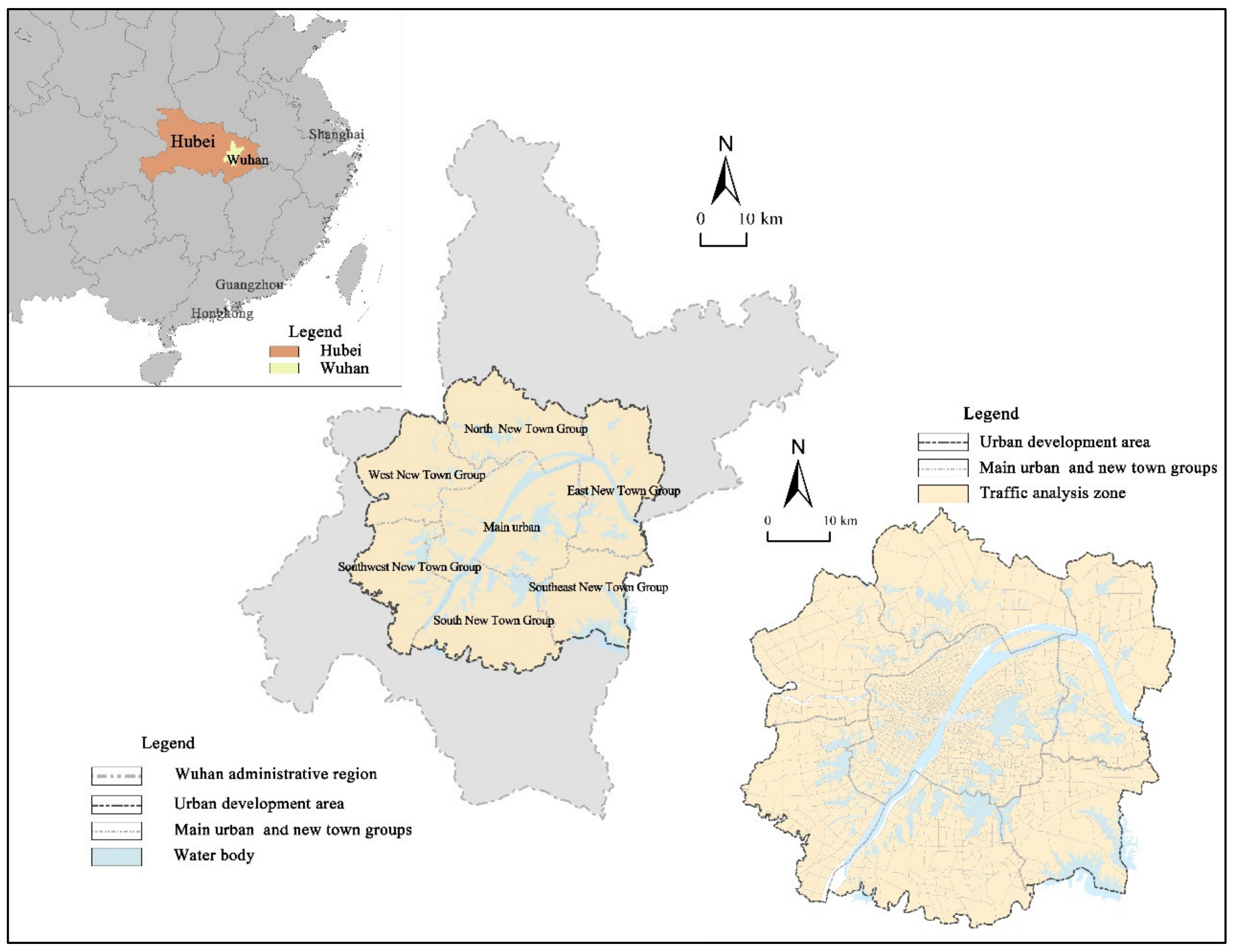
Although studies have focused on the interaction between the built environment and travel behavior, little is known about the relevant relationship in polycentric cities. In addition, the findings of studies on the impact of monocentric versus polycentric cities on commuting are not in agreement. Compared to other cities, Wuhan has a unique polycentric pattern of two rivers (the Yangtze and Hanshui Rivers) and three towns (Wuchang, Hankou, and Hanyang) due to the natural landscape pattern. Separated by these two rivers, Wuhan has a unique cross-river commuting behavior and commuters travel a relatively long distance.

3. Research Design

3.1. Study Area

We selected Wuhan, the largest city in central China, as the research object. The research scope covered the Wuhan urban development zone, as a typical polycentric city as it is divided by the Yangtze and Hanshui Rivers and contains three administrative districts, Wuchang, Hankou and Hanyang. The urban development zone is the agglomeration and expansion area of Wuhan’s urban functions, having a total area of 3261 km². According to Wuhan Territorial Spatial Planning (2021–2035), the urban spatial structure of the region is divided into one main urban area and six new town groups. As can be seen from Figure 1, the main urban area is the core agglomeration area of Wuhan, which contains the main employment locations and residential population of Wuhan. The six new town groups are the main expansion areas of Wuhan that have experienced the fastest growth in population and economic development in the recent years. Similar to other large cities, the rapid growth in population and employment along with the rapid expansion of urban areas has reshaped the travel demand of residents and caused urban issues such as traffic congestion and long commuting distances. Therefore, using Wuhan as the research object can better reflect the relationship between the built environment and commuting distance in polycentric cities, and the findings can provide policy implications for similar regions. In this study, we used the traffic analysis zone (TAZ) as the basic research unit, based on the geographical information of residences and workplaces.

3.2. Method

In response to the least squares method commonly used in past studies of the built environment and commuting distance, overfitting occurs when the data sample is small or values are missing. BLR can effectively prevent the occurrence of overfitting by introducing the Gaussian prior to achieve a penalty parameter (L2 norm) for the parameter w (vectors). Therefore, to more accurately analyze the impact of the TAZ built environment at both residential and job locations on commuting distances, we used the BLR model for analysis. From a Bayesian perspective, we constructed linear regressions using probability distributions rather than point estimates. The response variable y is not a single value being estimated but is assumed to be drawn from a normal distribution. The BLR model is as follows:

$$y~N({\beta }^{T}X,{\sigma }^{2}I)$$

(1)

where y is generated from a normal (Gaussian) distribution inscribed by both the mean and variance, and the variance is the square of the standard deviation σ.

Since the purpose of BLR is not to find a single best value for the model parameters, but to determine the posterior distribution of the model parameters, both the response variables and the model parameters are generated from a probability distribution. The posterior distributions of the model parameters are conditioned on the inputs and outputs of the training. Assuming the overall parameter y to be estimated, we randomly draw some data β from this population. The posterior probability is [13]:

$$P(\beta |y, X)=\frac{P\left(\beta |y, X\right)\ast P(\beta |X)}{P(\beta |X)}$$

(2)

where P (β|y, X) is the posterior probability distribution of the model parameters given the inputs and outputs; it is equal to the likelihood function P (y|β, X) of the output multiplied by the prior probability P (β|x) of the parameter β given the input, and divided by the normalized constant.

3.3. Data Sources and Description

The data used in this study included the Unicom cellular signaling data of Wuhan in June 2019; road, metro station and other vector data in Wuhan in 2019; POI data in Wuhan in 2019; and vector data of land use in Wuhan from 2016.

Among them, we obtained cellular signaling data from China Unicom, which records the encrypted unique user identification number, basic attributes of individual users, location latitude and longitude, and location point type and other information. The user location point types are catalogued as residence, employment and visiting by the duration and frequency of stay of the user at different time periods of the month. In this study, we selected the permanent users in Wuhan urban development zone to obtain the latitude and longitude coordinates of their residential and job locations as well as relevant individual attributes, and the users’ commuting distance was calculated through their residential and job location points. In order to eliminate the interference of outliers, the age of employed people was limited to 18–65 years old. In addition, cellular signaling data can be used to identify residential population density and employment population density. Vector data such as roads and metro stations, and the POI data of Wuhan were obtained through AMAP. AMAP’s POI covers various spatial geographic information (longitude and latitude, detailed address), as well as attribute information such as specific facility names and main categories, presented in the form of spatial points. The POI data of Wuhan were obtained from the API interface of AMAP, mainly including companies, metro stations, bus stops, and other public facilities related to residents’ job and housing. The land use data were obtained from Wuhan Planning and Design Institute. The land use data used in this study differed from other data by a certain number of years, but considering that their main use was for calculating the land use mix, that urban construction requires some time, and that most regions in Wuhan urban development zone are built-up areas, the impact of using these older data could be ignored. In addition, the use of official vector data can guarantee the accuracy of the results to a greater extent compared to the use of land use data converted from POI data, remote sensing data, etc.

In this study, the dependent variable was commuting distance (distance from residence to workplace), which was obtained from cellular signaling data. Distribution of commuting distance of residents in Wuhan urban development zone is shown in Figure 2. The average commuting distance of residents in Wuhan urban development zone was 7.52 km, which is lower than the average commuting distance of 8.2 km in Wuhan. The reason for this difference may be that the commuting distance measured in this study was the Euclidean distance from the residence to the workplace, whereas the average commuting distance in Wuhan is determined based on the shortest distance of the road network. In addition, even if the calculation is based on the Euclidean distance, the proportion of commuting distance within 5 km was still less than 50%. From the perspective of major cities in China, the average commuting distance in Wuhan is relatively long, ranking in the top ten among the major cities in China [34]. The main reason for this phenomenon is the natural pattern of Wuhan. As can be seen from Figure 3 and Figure 4, the employment centers in Wuhan are divided by the Yangtze and Hanshui Rivers, causing dislocation between job and housing locations, which results in a large number of cross-river commuters within Wuhan’s urban development zone. Among them, the proportion of cross-river commuters in the main city is the highest of all types, reaching 60%.

The independent variables were analyzed according to the residential and job locations identified for commuters, using TAZ as the basic unit and selecting 11 independent variables involving residents’ commuting behavior in the 5D elements of the built environment. The descriptive statistics of built environment within the research scope are provided in

Table 1. Descriptive statistics of built environment factors.

Variable		Description	Average	SD
Residential Built Environment Factors at the TAZ Level
Density	Residential density	Ratio of resident population obtained through cellular signaling data to TAZ (persons/km2).	6056.04	4921.28
	Employment density	Ratio of employed population obtained through cellular signaling data to TAZ (persons/ km2)	2150.34	2281.77
	Plot ratio	Plot ratio of each TAZ calculated through the building vector data of Wuhan.	0.46	1.87
Diversity	Land use mix	$S=\frac{-{{\displaystyle \sum }}_{i=1}^k{p}_i\ln p_i}{\ln k}$ where S is the land use mix; k is the classification data of land use types; $p_i$ is the proportion of land area in category I, ${{\displaystyle \sum }}_{i=1}^k{p}_i=1$	0.55	0.15
Design	Number of intersections	Number of intersections in each TAZ	24.00	30.10
	Parking service level	Number of parking lots in each TAZ	17.95	19.25
Destination	Number of companies	Number of corporate POIs in each TAZ	55.89	78.18
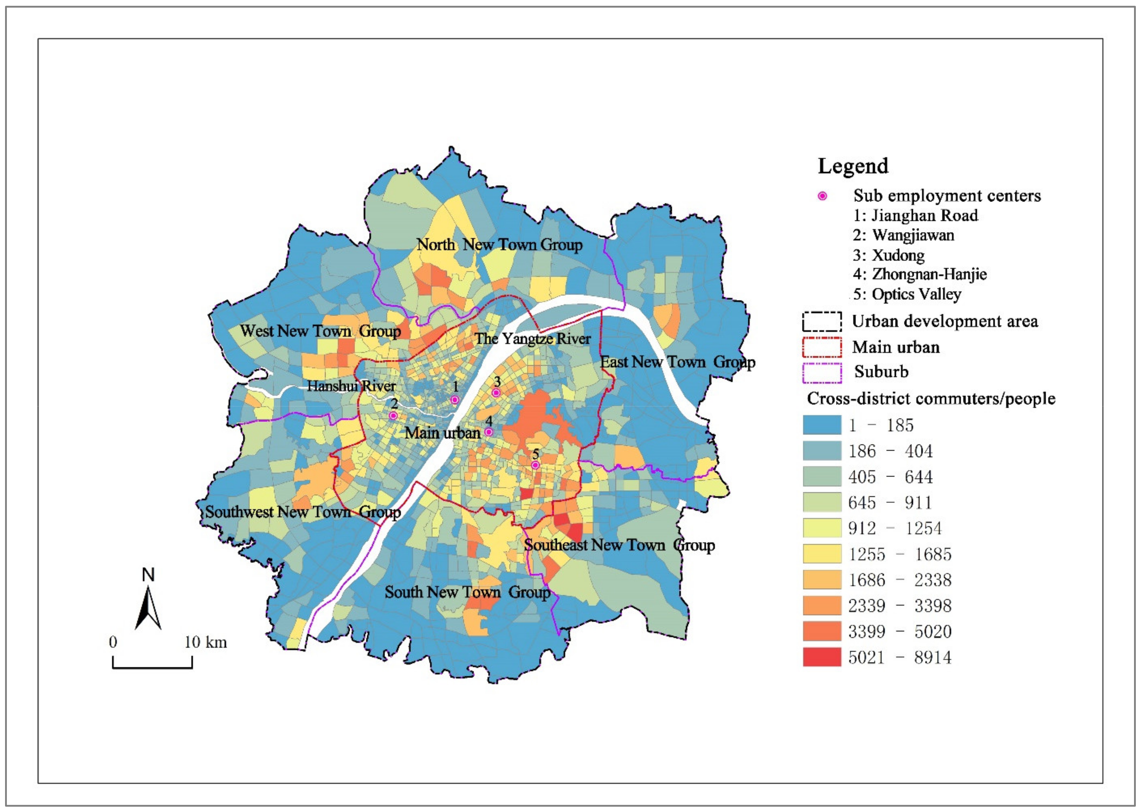
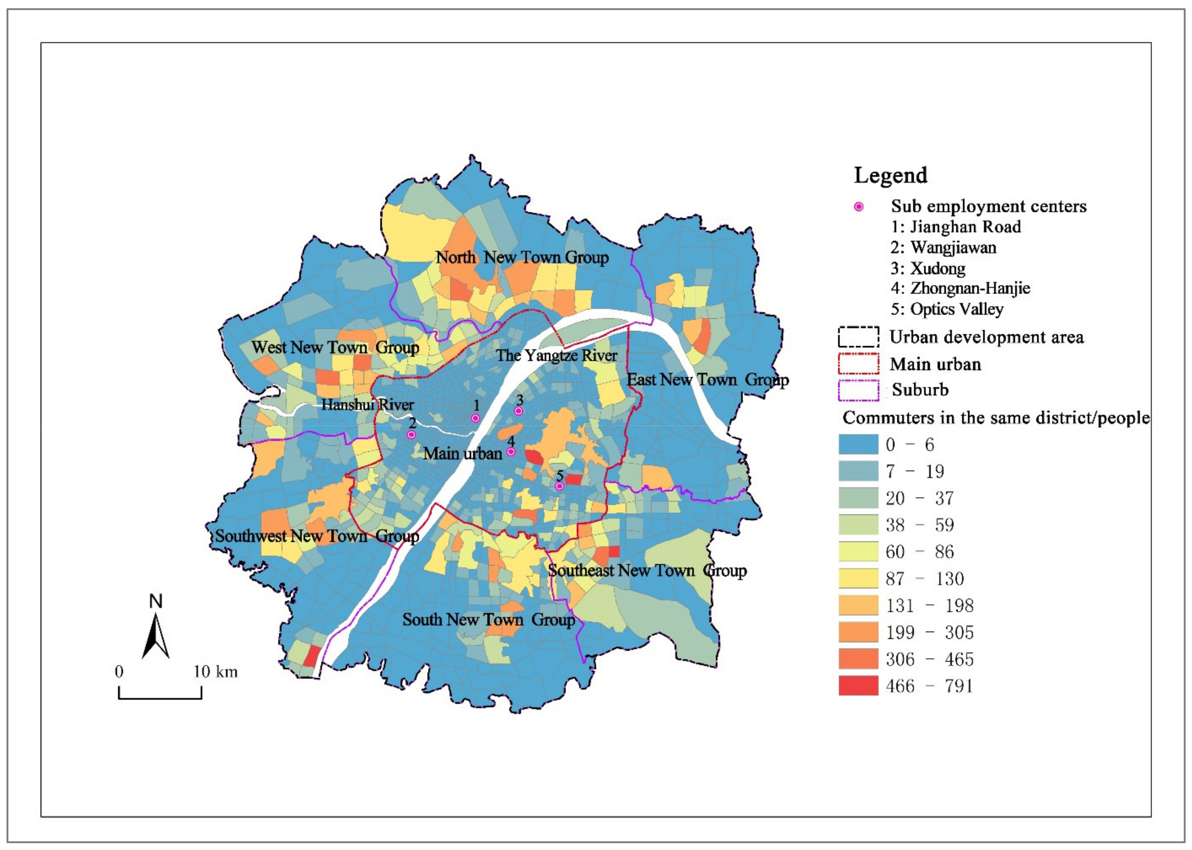
Distance	Distance to sub employment centers	Calculate the straight-line distance of individual residence from five employment centers in Wuhan (As shown in Figure 3, Jianghan Road, Wangjiawan, Xudong, Zhongnan-Hanjie, Optics Valley), and choose the smallest distance (km)	7162.21	5628.51
	Number of metro stations	Number of metro stations in each TAZ	0.21	0.48
	Number of bus stops	Number of bus stops in each TAZ	4.38	5.79
Workplace built environment factors at the TAZ level
Density	Residential density	Ratio of population obtained through cellular signaling data to TAZ (persons/km2).	6020.68	5094.84
	Employment density	Ratio of employed population obtained through cellular signaling data to TAZ (persons/ km2)	3236.79	3582.7
	Plot ratio	Plot ratio of each TAZ calculated through the building vector data of Wuhan.	0.44	1.31
Diversity	Land use mix	$S=\frac{-{{\displaystyle \sum }}_{i=1}^k{p}_i\ln p_i}{\ln k}$ where S is the land use mix; k is the classification data of land use types; $p_i$ is the proportion of land area in category I, ${\displaystyle \sum }_{i=1}^k{p}_i=1$	0.55	0.16
Design	Number of intersections	Number of intersections in each TAZ	23.83	30.18
	Parking service level	Number of parking lots in each TAZ	20.10	22.80
Destination	Number of companies	Number of corporate POIs in each TAZ	74.49	98.75
Distance	Distance to sub employment centers	Calculate the straight-line distance of individual residence from five employment centers in Wuhan (As shown in Figure 3, Jianghan Road, Wangjiawan, Xudong, Zhongnan-Hanjie, Optics Valley), and choose the smallest distance (km)	6987.51	5904.79
	Number of metro stations	Number of metro stations in each TAZ	0.22	0.48
	Number of bus stops	Number of bus stops in each TAZ	4.02	6.01

.

4. Results and Discussion

We used the rstanarm package in the R programing language to estimate the BLR models, which led to the results presented in

Table 2. Bayesian model results for commuting distance.

Parameter	Median	95%CI	pd	ROPE	ROPE_CI	Rhat	ESS
Residential Built Environment Factors at the TAZ Level
Residential density	−0.01	[−0.02, −0.01]	100%	[−718.15, 718.15]	100%	1.00	2370
Employment density	−0.00	[−0.01, 0.01]	81.03%	[−718.15, 718.15]	100%	1.00	2453
Plot ratio	24.34	[16.85, 31.73]	100%	[−718.15, 718.15]	100%	1.00	10,833
Land use mix	−196.47	[−288.60, −107.42]	100%	[−718.15, 718.15]	100%	1.00	7292
Number of intersections	−7.02	[−7.54, −6.48]	100%	[−718.15, 718.15]	100%	1.00	5757
Parking service level	−4.28	[−5.23, −3.34]	100%	[−718.15, 718.15]	100%	1.00	4069
Number of companies	−1.18	[−1.39, −0.96]	100%	[−718.15, 718.15]	100%	1.00	4575
Distance to sub employment centers	0.07	[0.07, 0.08]	100%	[−718.15, 718.15]	100%	1.00	3218
number of metro stations	169.47	[141.91, 197.76]	100%	[−718.15, 718.15]	100%	1.00	7330
number of bus stops	20.91	[17.57, 24.01]	100%	[−718.15, 718.15]	100%	1.00	3877
Workplace built environment factors at the TAZ level
Residential density	0.00	[−0.00, 0.01]	96.33%	[−718.15, 718.15]	100%	1.00	3105
Employment density	0.10	[0.09, 0.10]	100%	[−718.15, 718.15]	100%	1.00	3555
Plot ratio	4.40	[−6.53, 14.84]	78.22%	[−718.15, 718.15]	100%	1.00	9154
Land use mix	−825.29	[−913.29, −734.31]	100%	[−718.15, 718.15]	0%	1.00	8841
Number of intersections	5.18	[4.65, 5.71]	100%	[−718.15, 718.15]	100%	1.00	5345
Parking service level	−17.68	[−18.53, −16.88]	100%	[−718.15, 718.15]	100%	1.00	4267
Number of companies	−0.82	[−0.99, −0.65]	100%	[−718.15, 718.15]	100%	1.00	4176
Distance to sub employment centers	0.21	[0.20, 0.21]	100%	[−718.15, 718.15]	100%	1.00	2930
number of metro stations	84.77	[54.35, 114.28]	100%	[−718.15, 718.15]	100%	1.00	8576
number of bus stops	27.25	[24.54, 30.22]	100%	[−718.15, 718.15]	100%	1.00	5344

* A coefficient estimate for a variable represents the posterior mean of its parameter, and S.E. is its standard error. A credible interval for the estimate is bounded by l–95%CI and u-95%CI. If the 95%CI does not include zero, this variable is statistically significant at the 5% level.

. Since the objective of this study was to explore the effect of the built environment at residential and job locations on commuting distance, the analysis was conducted separately from the residential and the employment side according to Table 2.

In terms of built environment characteristics at residential locations, Table 2 shows that, similar to the results of existing studies [5,36], the built environment’s characteristics at residential location had a significant impact on commuting distance of residents. In general, factors, such as residential density, plot ratio, land use mix, number of intersections, number of companies, and distance to sub-employment centers, had a significant impact on commuting distance, which further confirmed that living in a compact and public-transport oriented built environment is conducive to reducing the commuting distance of residents. Specifically, residential density was negatively correlated with commuting distance, which is consistent with findings in Washington [10]. In addition, commuting distance and land use mix also showed significant negative effects, which is consistent with the findings of Sun et al. [26] and Antipova et al. [37]. This is because a more diverse land use mix allows residents to complete their daily life activities in a small geographical unit. According to a Shanghai-based study by Sun et al. [26], intersection density was positively correlated with private car commuting and negatively correlated with public transport commuting, whereas Zhang’s [25] Boston and Hong Kong-based study found that intersection density helps reduce the likelihood of commuting by car. In our study, we found that overall intersection density contributed to shorter commuting distances. This may be because the higher the intersection density, the higher the road density, which can provide more flexible and convenient commuting routes, thus contributing to the reduction in commuting distance. We also found that distance to sub-employment centers was positively correlated with commuting distance, which is due to most employment opportunities being concentrated in sub-employment centers in cities with a polycentric layout. To some extent, residing far away from sub-employment centers means being far away from the workplace. Our findings support the idea that the polycentric urban spatial structure development pattern is conducive to lower commuting distances. In addition, we found that the numbers of bus stops and metro stations were positively correlated with commuting distance, which may be due to public transportation providing more options for residential and job locations, which, to some extent, exacerbates the regional job–housing imbalance and thus increases the commuting distance for residents. In contrast to the findings of other studies [17,21], commuting distance and plot ratio showed positive effects. The reason for this finding may be that the plot ratio of Wuhan is gradually decreasing from the main city to the edge, showing an obvious core edge structure. In the descriptive analysis, we stated that a large number of cross-river commuters exist in the main city of Wuhan due to the influence of the natural geographical pattern, resulting in a relatively long commuting distance. However, in the six new town groups, the plot ratio was relatively low, and under the polycentric urban spatial structure of Wuhan, a large number of people worked in the nearest sub-employment center, so their commuting distance was relatively short.

In terms of built environment characteristics at job locations, the number of intersections, distance to sub employment centers, number of metro stations, and the number of bus stops had a significant positive effect on commuting distance, while land use mix, parking service level and number of companies had a significant negative effect. A comparison with residential locations revealed that the impact of land use mix at job locations was significantly higher than at residential locations, so the land use mix at job locations appears to play a dominant role in influencing commuting distance. The impact of parking service level at job locations was also higher than at residential location, suggesting that increasing the number of parking spaces at the workplace is more conducive to residents using private cars for commuting and increases commuting distance. In addition, the numbers of metro stations and bus stops showed heterogeneity in residential and job locations, with the number of metro stations having a more significant impact in residential areas, and while the number of bus stops having a stronger impact in employment areas. The reason for this finding is that the metro construction in Wuhan is still in the early and middle stages, the metro network already covers all employment centers, but the coverage of the residential locations is somewhat insufficient. Ground public transportation, in comparison, is a more mature service and has basically achieved full coverage of the main city. Therefore, the impact of the metro is stronger at residential locations, and that of public transport at job location is more obvious. Notably, the number of intersections had a negative effect on commuting distance at residential locations, but a positive effect at job locations. This is similar to the findings of Sun et al. [26], where road network density at job locations was found to encourage private car commuting, but the spatial concentration of workspaces had the potential to increase traffic congestion and increase commuting distance.

5. Conclusions

In recent years, the negative effects of increased commuting distances, traffic congestion, and the resulting air pollution caused by global urban sprawl have driven research on the built environment and commuting behavior. Understanding the impact of the built environment on commuting distance can help planning decision makers reduce commuting distance and cost at the micro level, which in turn reduces energy consumption, traffic emissions, and air pollution. We based our study on BLR to explore the impact of the built environment at both residential and job locations on commuting distance: we considered job location to examine the impact of the built environment on commuting distance, which is different from most of the previous studies, and we used BLR to address the problem of overfitting experienced with traditional linear regression. In addition, individual commuting distance measures based on cellular signaling data provided an objective and indicator of residents’ commuting distance. Our study shows that differences exist in the impacts of built environment at residential and job locations on commuting distance, which provides new findings on the effects of built environments on commuting distance at the TAZ level. The findings provide a more detailed and scientific reference for the optimization of built environments at the micro level.

Taking the Wuhan urban development zone in China as the research object, we found that, at the TAZ level, the built environment at both residential and job locations had a significant impact on residents’ commuting distance. Specifically, for residential locations, five factors (residential density, land use mix, number of intersections, parking service level, and number of companies) had a significant negative effect on commuting distance, while four factors (plot ratio, distance to sub employment centers, number of metro stations, and number of bus stops) had a significant positive effect on commuting distance. For employment locations, three factors (land use mix, parking service level, and number of companies) had a significant negative effect on commuting distance, while five factors (job density, number of intersections, distance to sub-employment centers, number of metro stations, and number of bus stops) had a significant positive effect on commuting distance. Our study further confirms that living in a city that is compact and functionally complex in land-use is conducive to reducing residents’ commuting distance. However, land use mix appears to have a significantly stronger impact on reducing commuting distance in job locations than in residential locations, and metro and bus stops have a greater impact at residential and job locations, respectively. In addition, distance to sub-employment centers showed a significant positive effect on commuting distance at both residential and job locations, and our findings support the idea that polycentric urban development is beneficial to reducing residents’ commuting distance. However, as pointed out by Hu et al. [1], polycentric development in large cities needs to provide suitable housing and public services for new employment centers to avoid the increase in commuting distance caused by job and housing imbalances.

However, this study has certain limitations that warrant further research. First, the commuting distance of residents measured in this study based on cellular signaling data is the Euclidean distance, which is not the real commuting distance, so this may have had some influence on the research results. With the increasing popularity of big data, we encourage the measurement of commuting distance based on residents’ real commuting trajectories in the future to obtain more accurate results. In addition, due to data limitations, we did not consider different travel modes. However, as found by Sun et al. [26] and others, differences may exist in the effects of changes in the built environment on different travel modes. As our goal is to shorten commuting distance and encourage the use of public transportation, increasing the research on different travel modes can be considered in future research, which would, in turn, lead to suggestions of more targeted built environment optimization measures. In addition, residents’ socioeconomic attribute characteristics and travel preferences can also impact residents’ commuting distance, and future studies need to add individual data to address the impact of the built environment and residents’ self-selection on commuting distance [26,38]. Furthermore, although we identified the factors of the built environment at both residential and job locations influencing commuting distances, knowing the thresholds of built environment variables will be more beneficial to planning practice and the formulation of related policies [39,40], and we suggest the introduction of machine learning (such as Gradient Boosting Decision Tree) and other methods to solve the problem in the future.

References

- Hu, L.; Sun, T.; Wang, L. Evolving urban spatial structure and commuting patterns: A case study of Beijing, China. Transp. Res. Part D Transp. Environ. 2018, 59, 11–22. [Google Scholar] [CrossRef]
- Ewing, R.; Cervero, R. Travel and the built environment. J. Am. Plan. Assoc. 2010, 76, 265–294. [Google Scholar] [CrossRef]
- Ewing, R.; Cervero, R. Travel and the Built Environment: A Synthesis. Transp. Res. Rec. 2001, 87–114. [Google Scholar] [CrossRef] [Green Version]
- Ding, C.; Mishra, S.; Lu, G.; Yang, J.; Liu, C. Influences of built environment characteristics and individual factors on commuting distance: A multilevel mixture hazard modeling approach. Transp. Res. Part D Transp. Environ. 2017, 51, 314–325. [Google Scholar] [CrossRef]
- Manaugh, K.; Miranda-Moreno, L.F.; El-Geneidy, A.M. The effect of neighbourhood characteristics, accessibility, home-work location, and demographics on commuting distances. Transportation 2010, 37, 627–646. [Google Scholar] [CrossRef]
- Guo, J.Y.; Chen, C. The built environment and travel behavior: Making the connection. Transportation 2007, 34, 529–533. [Google Scholar] [CrossRef]
- Handy, S. Is accessibility an idea whose time has finally come? Transp. Res. Part D Transp. Environ. 2020, 83, 102319. [Google Scholar] [CrossRef]
- Yang, L.; Ding, C.; Ju, Y.; Yu, B. Driving as a commuting travel mode choice of car owners in urban China: Roles of the built environment. Cities 2021, 112, 103114. [Google Scholar] [CrossRef]
- Ye, R.; Titheridge, H. Satisfaction with the commute: The role of travel mode choice, built environment and attitudes. Transp. Res. Part D Transp. Environ. 2017, 52, 535–547. [Google Scholar] [CrossRef]
- Ding, C.; Cao, X. How does the built environment at residential and work locations affect car ownership? An application of cross-classified multilevel model. J. Transp. Geogr. 2019, 75, 37–45. [Google Scholar] [CrossRef]
- Bai, X.; Zhai, W.; Steiner, R.L.; He, Z. Exploring extreme commuting and its relationship to land use and socioeconomics in the central Puget Sound. Transp. Res. Part D Transp. Environ. 2020, 88, 102574. [Google Scholar] [CrossRef]
- Chen, E.; Ye, Z.; Bi, H. Incorporating smart card data in spatio-temporal analysis of metro travel distances. Sustainability 2019, 11, 7069. [Google Scholar] [CrossRef] [Green Version]
- Efron, B. Bayes’ theorem in the 21st century. Science 2013, 340, 1177–1178. [Google Scholar] [CrossRef] [PubMed]
- Lombardo, L.; Cama, M.; Conoscenti, C.; Märker, M.; Rotigliano, E. Binary logistic regression versus stochastic gradient boosted decision trees in assessing landslide susceptibility for multiple-occurring landslide events: Application to the 2009 storm event in Messina (Sicily, southern Italy). Nat. Hazards 2015, 79, 1621–1648. [Google Scholar] [CrossRef]
- Yang, L.; Liu, J.; Liang, Y.; Lu, Y.; Yang, H. Spatially varying effects of street greenery on walking time of older adults. ISPRS Int. J. Geo-Information 2021, 10, 596. [Google Scholar] [CrossRef]
- Cervero, R. Alternative approaches to modeling the travel-demand impacts of smart growth. J. Am. Plan. Assoc. 2006, 72, 285–295. [Google Scholar] [CrossRef]
- Zhao, P. The Impact of the Built Environment on Individual Workers’ Commuting Behavior in Beijing. Int. J. Sustain. Transp. 2013, 7, 389–415. [Google Scholar] [CrossRef]
- Ding, C.; Lin, Y.; Liu, C. Exploring the influence of built environment on tour-based commuter mode choice: A cross-classified multilevel modeling approach. Transp. Res. Part D Transp. Environ. 2014, 32, 230–238. [Google Scholar] [CrossRef]
- Kemperman, A.; Timmerman, H. Influences of built environment on walking and cycling by latent segments of aging population. Transp. Res. Rec. 2009, 2134, 1–9. [Google Scholar] [CrossRef]
- Kuby, M.; Barranda, A.; Upchurch, C. Factors influencing light-rail station boardings in the United States. Transp. Res. Part A Policy Pract. 2004, 38, 223–247. [Google Scholar] [CrossRef]
- Cervero, R.; Kockelman, K. Travel demand and the 3Ds: Density, diversity, and design. Transp. Res. Part D Transp. Environ. 1997, 2, 199–219. [Google Scholar] [CrossRef]
- Bezirgani, A.; Lachapelle, U. Online grocery shopping for the elderly in Quebec, Canada: The role of mobility impediments and past online shopping experience. Travel Behav. Soc. 2021, 25, 133–143. [Google Scholar] [CrossRef]
- Böcker, L.; van Amen, P.; Helbich, M. Elderly travel frequencies and transport mode choices in Greater Rotterdam, the Netherlands. Transportation 2017, 44, 831–852. [Google Scholar] [CrossRef] [Green Version]
- Spinney, J.E.L.; Scott, D.M.; Newbold, K.B. Transport mobility benefits and quality of life: A time-use perspective of elderly Canadians. Transp. Policy 2009, 16, 1–11. [Google Scholar] [CrossRef]
- Zhang, M. The role of land use in travel mode choice: Evidence from Boston and Hong Kong. J. Am. Plan. Assoc. 2004, 70, 344–360. [Google Scholar] [CrossRef]
- Sun, B.; Ermagun, A.; Dan, B. Built environmental impacts on commuting mode choice and distance: Evidence from Shanghai. Transp. Res. Part D Transp. Environ. 2017, 52, 441–453. [Google Scholar] [CrossRef]
- Ding, C.; Cao, X.; Liu, C. How does the station-area built environment influence Metrorail ridership? Using gradient boosting decision trees to identify non-linear thresholds. J. Transp. Geogr. 2019, 77, 70–78. [Google Scholar] [CrossRef]
- Yang, J.; Su, P.; Cao, J. On the importance of Shenzhen metro transit to land development and threshold effect. Transp. Policy 2020, 99, 1–11. [Google Scholar] [CrossRef]
- Vasanen, A. Functional Polycentricity: Examining Metropolitan Spatial Structure through the Connectivity of Urban Sub-centres. Urban Stud. 2012, 49, 3627–3644. [Google Scholar] [CrossRef]
- Hu, L.; Yang, J.; Yang, T.; Tu, Y.; Zhu, J. Urban Spatial Structure and Travel in China. J. Plan. Lit. 2020, 35, 6–24. [Google Scholar] [CrossRef]
- Lin, T.; Xia, J.; Robinson, T.P.; Goulias, K.G.; Church, R.L.; Olaru, D.; Tapin, J.; Han, R. Spatial analysis of access to and accessibility surrounding train stations: A case study of accessibility for the elderly in Perth, Western Australia. J. Transp. Geogr. 2014, 39, 111–120. [Google Scholar] [CrossRef] [Green Version]
- Truong, L.T.; Somenahalli, S.V.C. Exploring frequency of public transport use among older adults: A study in Adelaide, Australia. Travel Behav. Soc. 2015, 2, 148–155. [Google Scholar] [CrossRef]
- Szeto, W.Y.; Yang, L.; Wong, R.C.P.; Li, Y.C.; Wong, S.C. Spatio-temporal travel characteristics of the elderly in an ageing society. Travel Behav. Soc. 2017, 9, 10–20. [Google Scholar] [CrossRef] [Green Version]
- Wong, R.C.P.; Szeto, W.Y.; Yang, L.; Li, Y.C.; Wong, S.C. Public transport policy measures for improving elderly mobility. Transp. Policy 2018, 63, 73–79. [Google Scholar] [CrossRef] [Green Version]
- Xiao, W.; Li, H.; Wei, Y.D. Understanding jobs-housing imbalance in urban China: A case study of Shanghai. J. Transp. Land Use 2021, 14, 389–415. [Google Scholar] [CrossRef]
- Ding, C.; Cao, X.; Wang, Y. Synergistic effects of the built environment and commuting programs on commute mode choice. Transp. Res. Part A Policy Pract. 2018, 118, 104–118. [Google Scholar] [CrossRef]
- Antipova, A.; Wang, F.; Wilmot, C. Urban land uses, socio-demographic attributes and commuting: A multilevel modeling approach. Appl. Geogr. 2011, 31, 1010–1018. [Google Scholar] [CrossRef]
- Cao, J. Examining the Relationship Between Neighborhood Built Environment and Travel Behavior: A Review from the US Perspective. Urban Plan. Int. 2015, 30, 46–52. [Google Scholar]
- Ding, C.; Cao, X.; Næss, P. Applying gradient boosting decision trees to examine non-linear effects of the built environment on driving distance in Oslo. Transp. Res. Part A Policy Pract. 2018, 110, 107–117. [Google Scholar] [CrossRef]
- Yang, J.; Cao, J.; Zhou, Y. Elaborating non-linear associations and synergies of subway access and land uses with urban vitality in Shenzhen. Transp. Res. Part A Policy Pract. 2021, 144, 74–88. [Google Scholar] [CrossRef]