
Classification of Floods in Europe and North America with Focus on Compound Events


Abstract
:1. Introduction
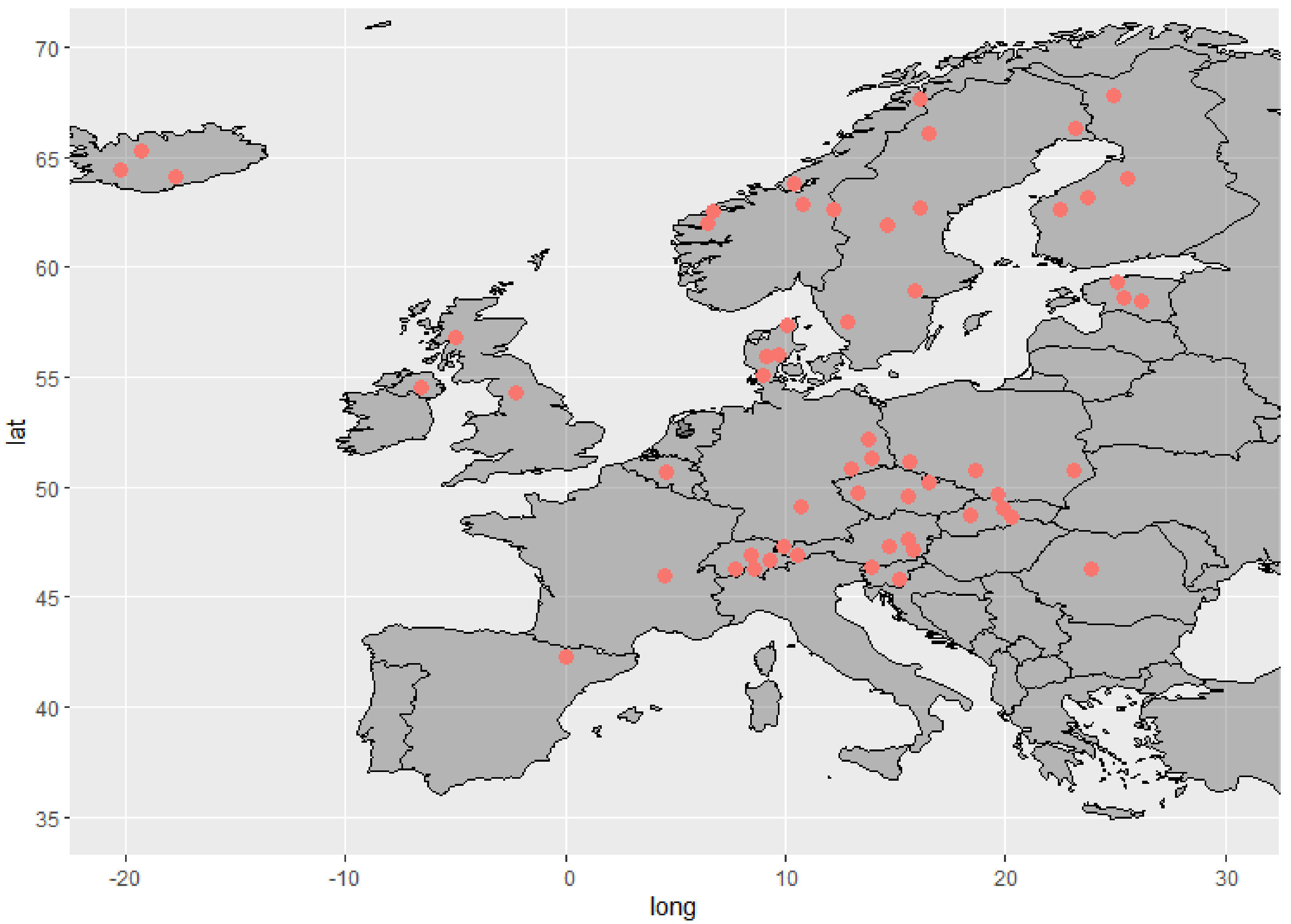
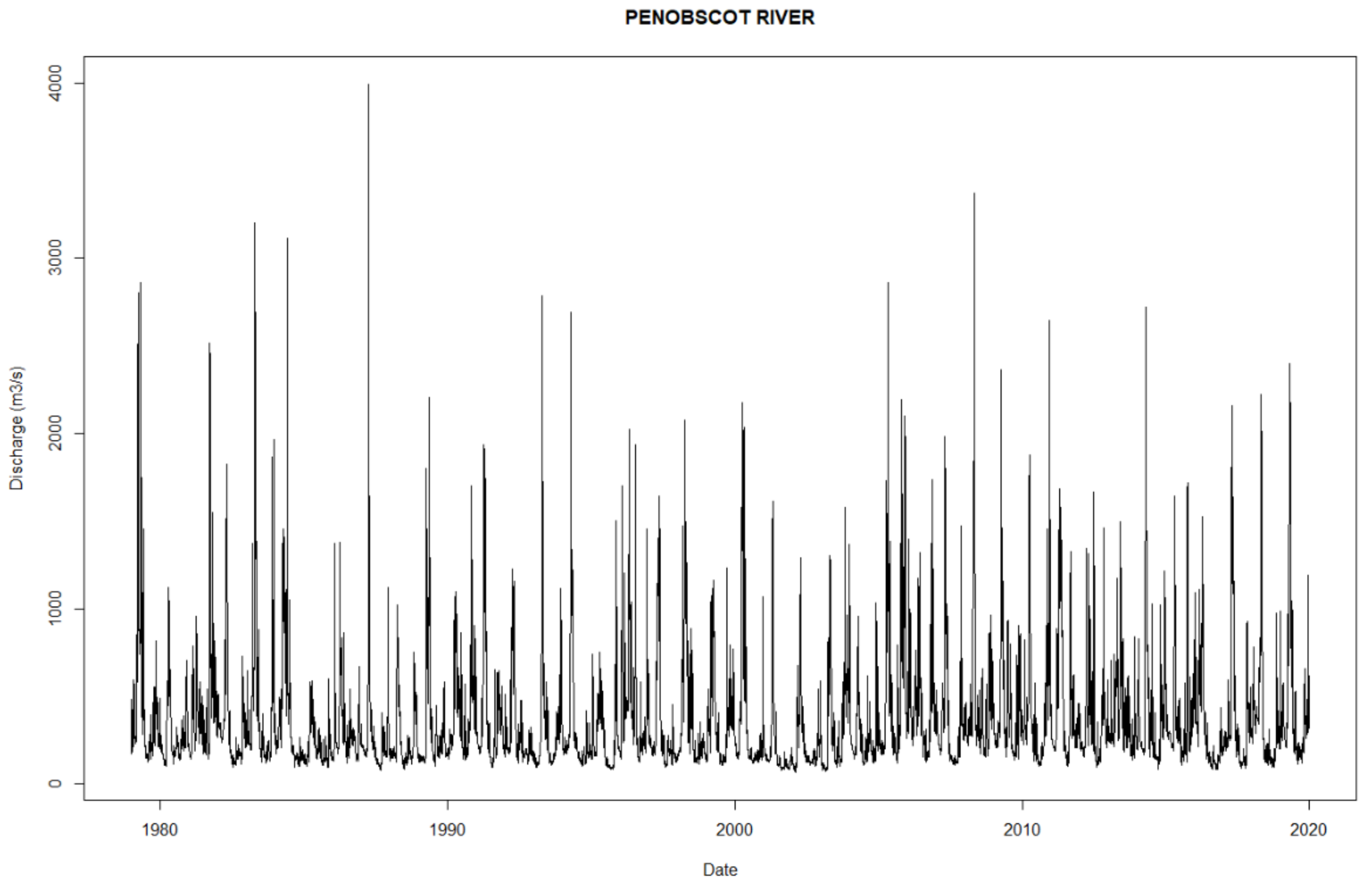
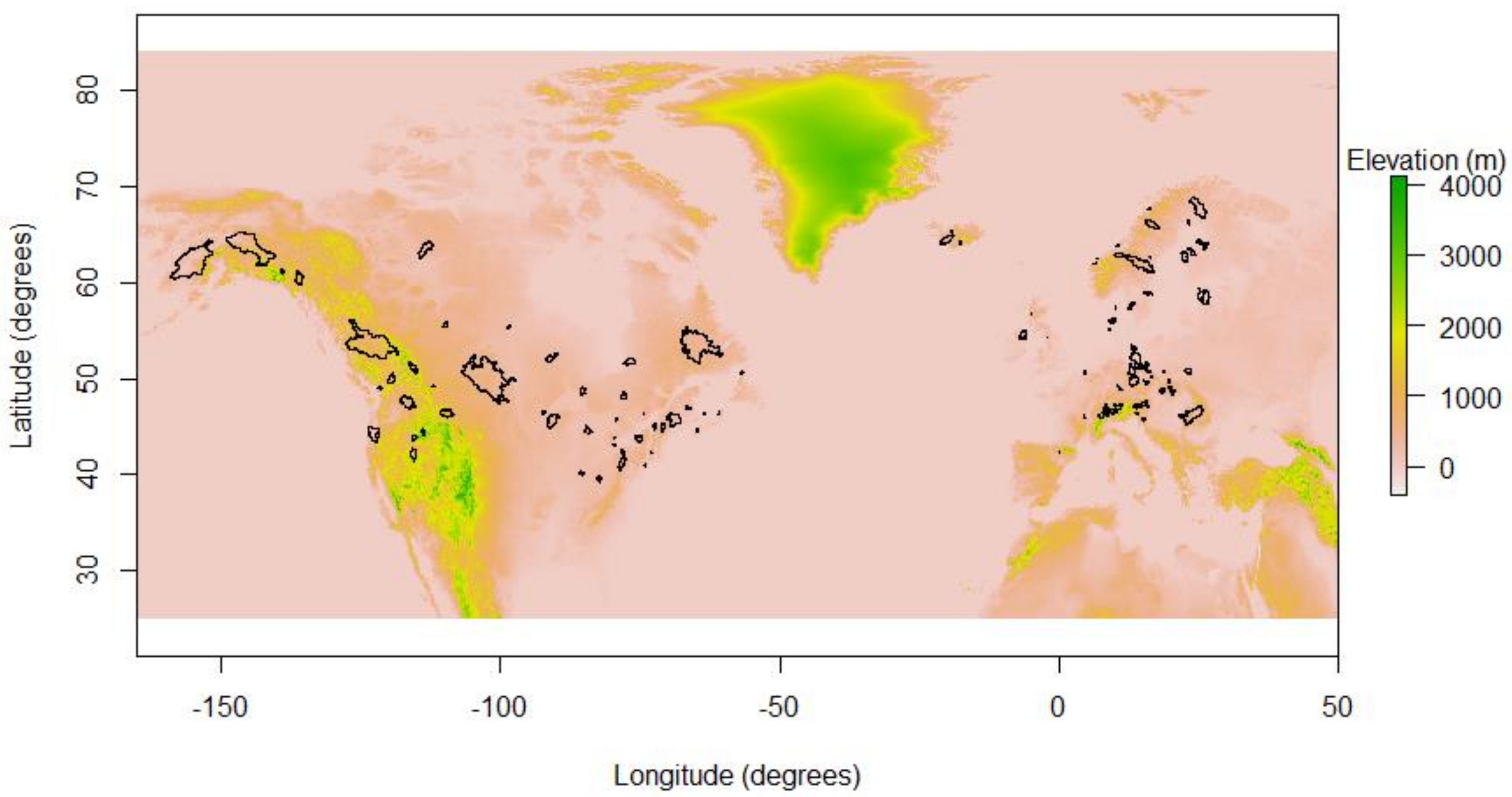
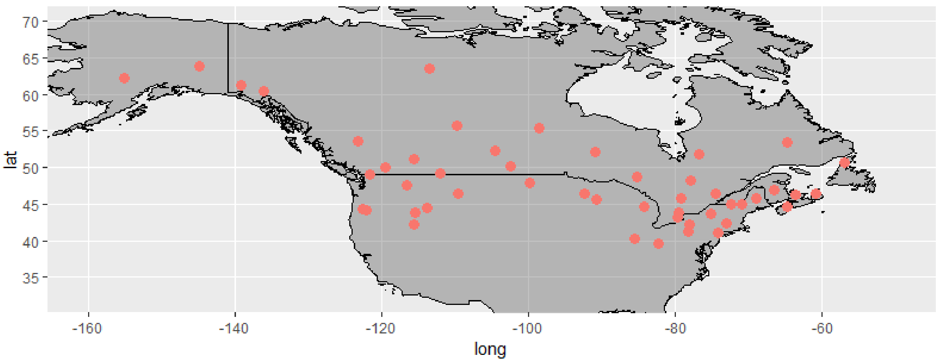
2. Data
3. Methods
3.1. Flood Hydrograph Seperation
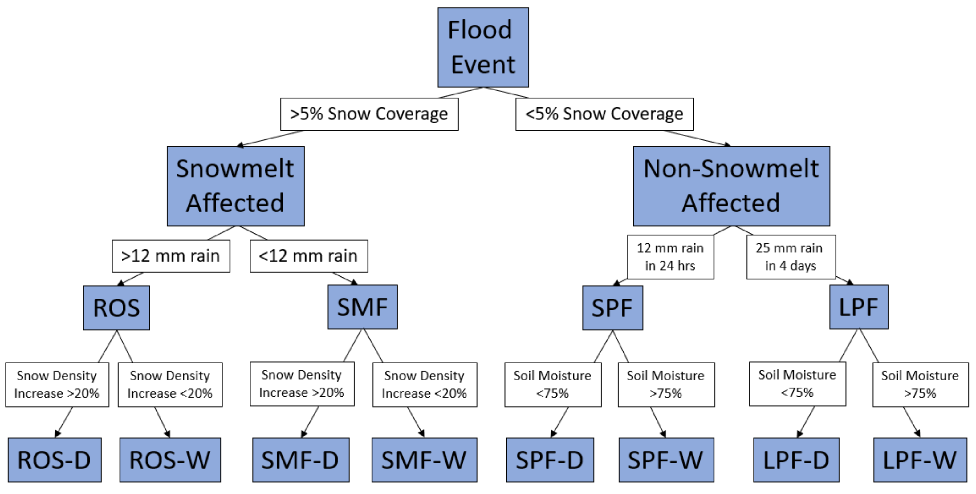
3.2. Flood Typology

| Flood Type | Precipitation [14] | Snow Cover [14] | Snowmelt [14] | Antecedent Moisture Condition | Other [36] | Abbreviation |
|---|---|---|---|---|---|---|
| Rain-on-Snow Flood with Dry Conditions | >12 mm | >5% | >1 mm | >20% Increase in snow density [35] | ROS-D | |
| Rain-on-Snow Flood with Wet Conditions | >12 mm | >5% | >1 mm | <20% Increase in snow density [35] | ROS-W | |
| Snowmelt Flood with Dry Conditions | <12 mm | >5% | >1 mm | >20% Increase in snow density [35] | SMF-D | |
| Snowmelt Flood with Wet Conditions | <12 mm | >5% | >1 mm | <20% Increase in snow density [35] | SMF-W | |
| Long-Precipitation Floods with Dry Conditions | >25 mm over 4 days | <5% | <1 mm | <75% soil saturation at start of hydrograph | Multiple Peaks | LPF-D |
| Long-Precipitation Floods with Wet Conditions | >25 mm over 4 days | <5% | <1 mm | >75% soil saturation at start of hydrograph | Multiple Peaks | LPF-W |
| Short-Precipitation Floods with Dry Conditions | >12 mm in 1 day | <5% | <1 mm | <75% soil saturation at start of hydrograph | SPF-D | |
| Short-Precipitation Floods with Wet Conditions | >12 mm in 1 day | <5% | <1 mm | >75% soil saturation at start of hydrograph | SPF-W |
4. Results and Discussion
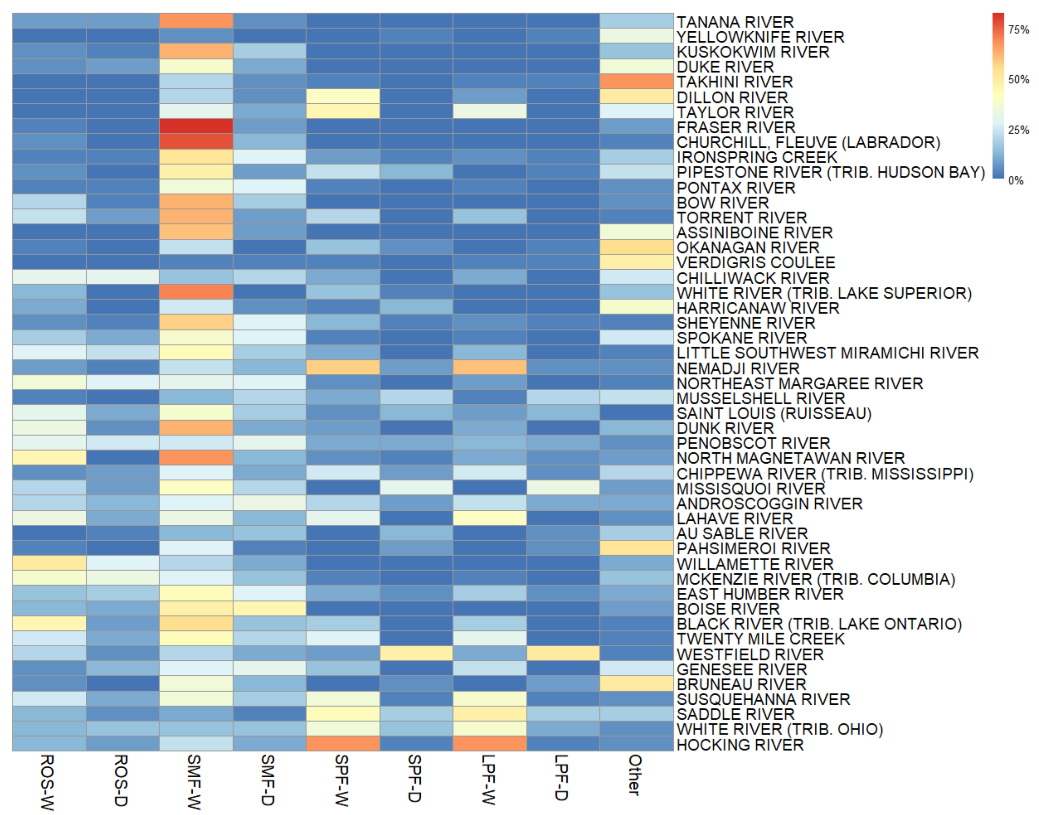
4.1. Flood Typology Classification for All Catchments
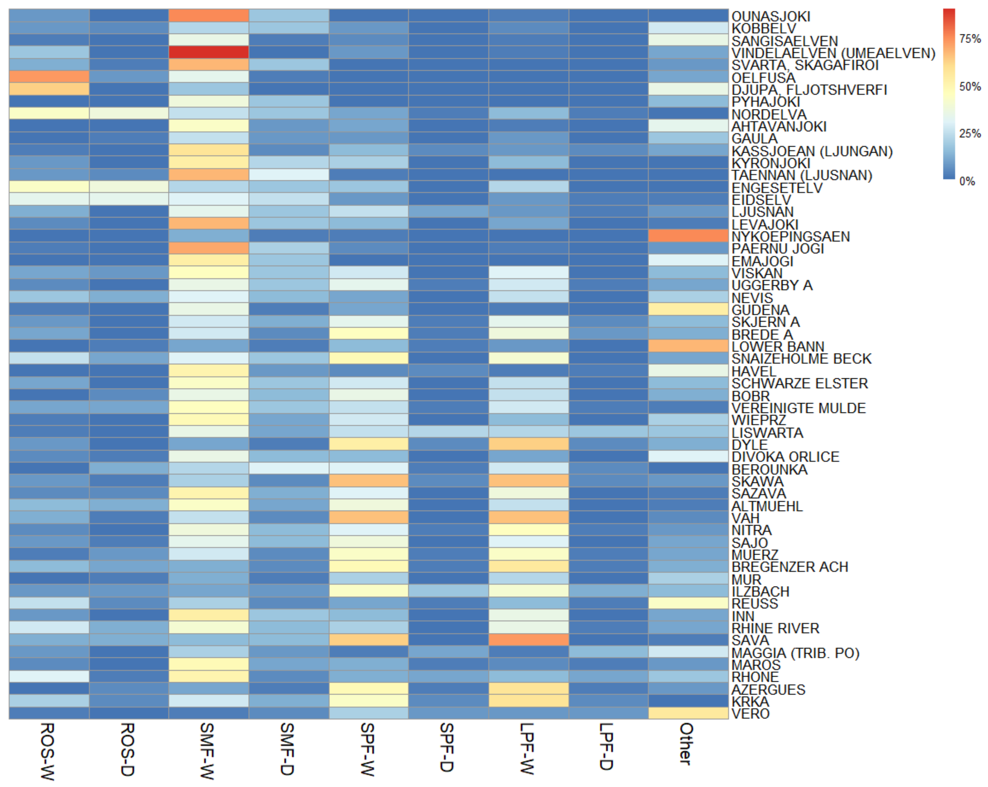
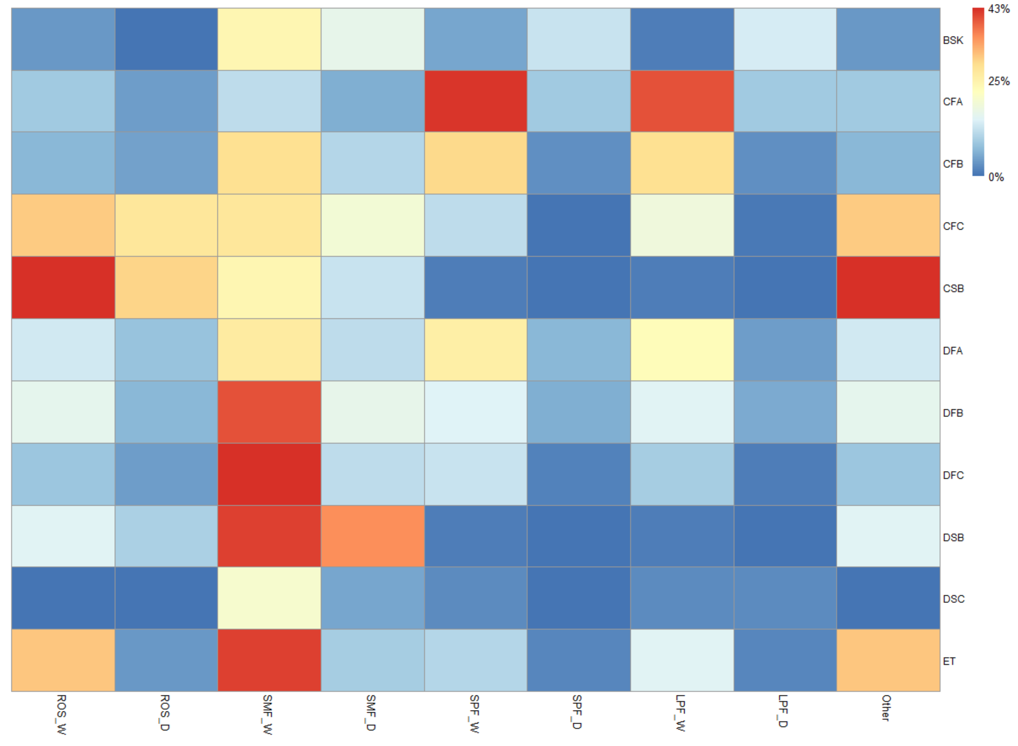
4.2. Flood Typology Classification Based on Climate Zone
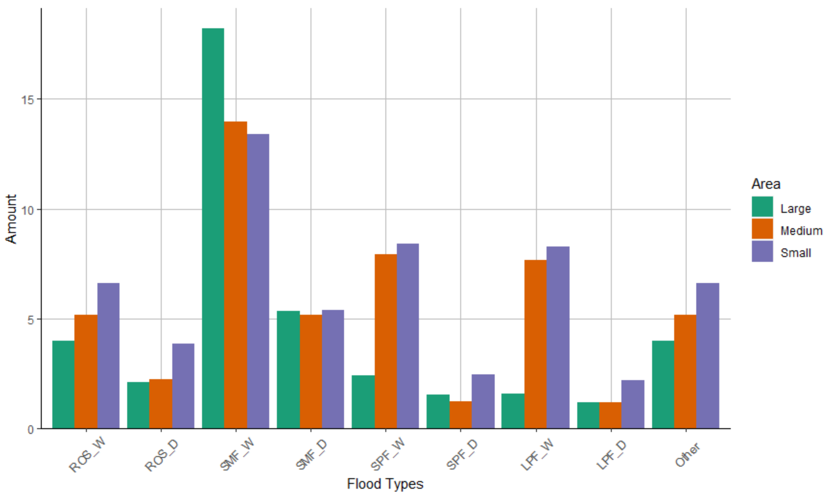
4.3. Flood Typology Classification Based on Catchment Area
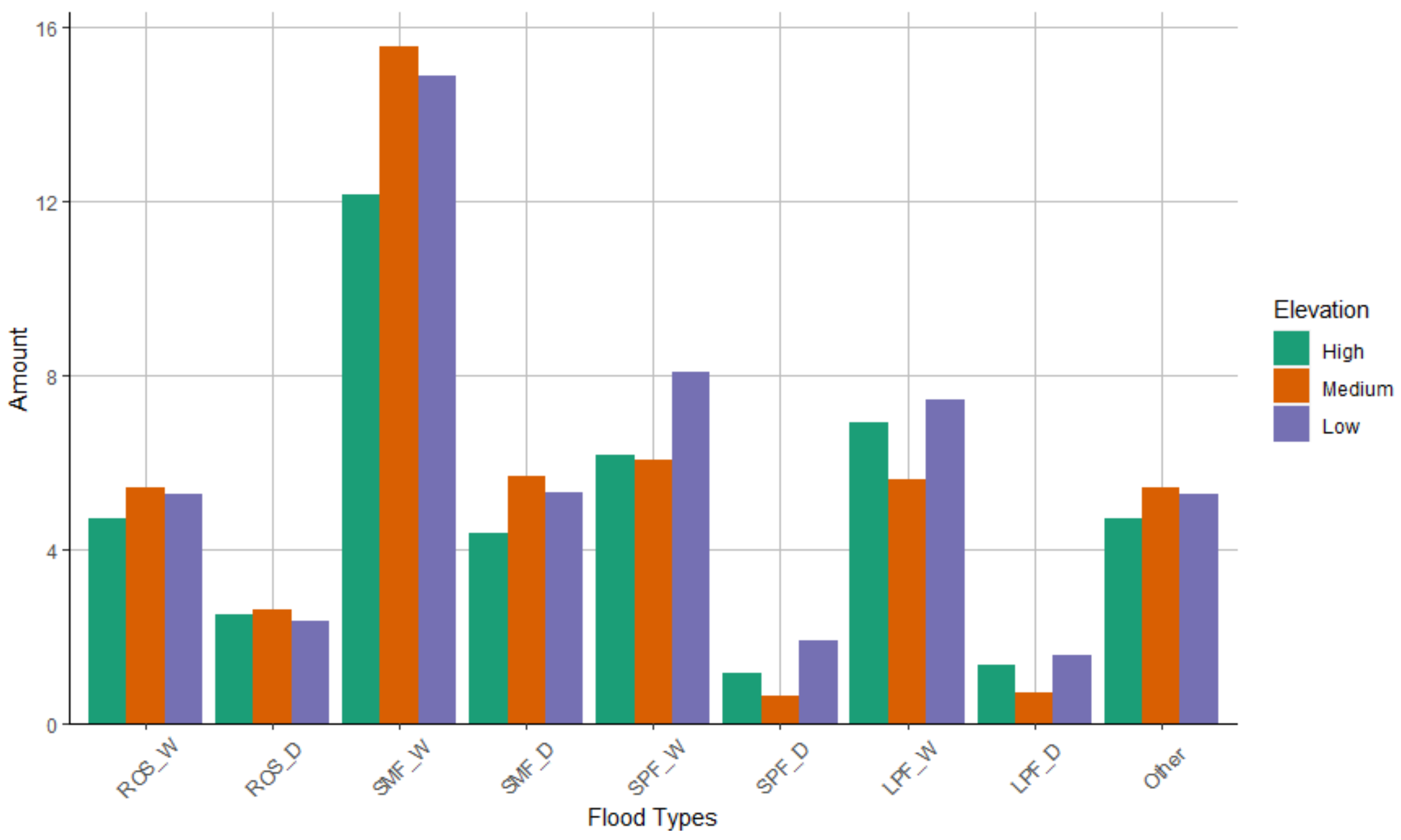
4.4. Flood Typology Classification Based on Elevation
5. Conclusions
Supplementary Materials
Author Contributions
Funding
Data Availability Statement
Conflicts of Interest
References
- Zscheischler, J.; Martius, O.; Westra, S.; Bevacqua, E.; Raymond, C.; Horton, R.M.; van den Hurk, B.; AghaKouchak, A.; Jézéquel, A.; Mahecha, M.D.; et al. A typology of compound weather and climate events. Nat. Rev. Earth Environ. 2020, 1, 333–347. [Google Scholar] [CrossRef]
- Wachowicz, L.J.; Mote, T.L.; Henderson, G.R. A rain on snow climatology and temporal analysis for the eastern United States. Phys. Geogr. 2020, 41, 54–69. [Google Scholar] [CrossRef]
- Sezen, C.; Šraj, M.; Medved, A.; Bezak, N. Investigation of rain-on-snow floods under climate change. Appl. Sci. 2020, 10, 1242. [Google Scholar] [CrossRef] [Green Version]
- Sutanto, S.J.; Vitolo, C.; Di Napoli, C.; D’Andrea, M.; Van Lanen, H.A.J. Heatwaves, droughts, and fires: Exploring compound and cascading dry hazards at the pan-European scale. Environ. Int. 2020, 134, 105276. [Google Scholar] [CrossRef] [PubMed]
- Bezak, N.; Mikoš, M. Changes in the compound drought and extreme heat occurrence in the 1961–2018 period at the european scale. Water 2020, 12, 3543. [Google Scholar] [CrossRef]
- Mikoš, M.; Četina, M.; Brilly, M. Hydrologic conditions responsible for triggering the Stože landslide, Slovenia. Eng. Geol. 2004, 73, 193–213. [Google Scholar] [CrossRef]
- Mikoš, M. After 2000 Stože landslide: Part II—Development in landslide disaster risk reduction policy in Slovenia—Po zemeljskem plazu Stože leta 2000: Del II—Razvoj politike zmanjševanja tveganja nesreč zaradi zemeljskih plazov v Sloveniji. Acta Hydrotech. 2021, 34, 39–59. [Google Scholar] [CrossRef]
- Mikoš, M. After 2000 Stože landslide: Part I—Development in landslide research in Slovenia—Po zemeljskem plazu Stože leta 2000: Del I—Razvoj raziskovanja zemeljskih plazov v Sloveniji. Acta Hydrotech. 2020, 33, 129–153. [Google Scholar] [CrossRef]
- Berghuijs, W.R.; Allen, S.T.; Harrigan, S.; Kirchner, J.W. Growing Spatial Scales of Synchronous River Flooding in Europe. Geophys. Res. Lett. 2019, 46, 1423–1428. [Google Scholar] [CrossRef] [Green Version]
- Bezak, N.; Borrelli, P.; Panagos, P. A first assessment of rainfall erosivity synchrony scale at pan-European scale. Catena 2021, 198, 105060. [Google Scholar] [CrossRef]
- Dietze, M.; Bell, R.; Ozturk, U.; Cook, K.L.; Andermann, C.; Beer, A.R.; Damm, B.; Lucia, A.; Fauer, F.S.; Nissen, K.M.; et al. More than heavy rain turning into fast-flowing water—A landscape perspective on the 2021 Eifel floods. Nat. Hazards Earth Syst. Sci. 2022, 22, 1845–1856. [Google Scholar] [CrossRef]
- Brunner, M.I.; Viviroli, D.; Sikorska, A.E.; Vannier, O.; Favre, A.-C.; Seibert, J. Flood type specific construction of synthetic design hydrographs. Water Resour. Res. 2017, 53, 1390–1406. [Google Scholar] [CrossRef] [Green Version]
- Poschlod, B.; Zscheischler, J.; Sillmann, J.; Wood, R.R.; Ludwig, R. Climate change effects on hydrometeorological compound events over southern Norway. Weather Clim. Extrem. 2020, 28, 100253. [Google Scholar] [CrossRef]
- Sikorska, A.E.; Viviroli, D.; Seibert, J. Flood-type classification in mountainous catchments using crisp and fuzzy decision trees. Water Resour. Res. 2015, 51, 7959–7976. [Google Scholar] [CrossRef]
- Merz, R.; Blöschl, G. A process typology of regional floods. Water Resour. Res. 2003, 39, 1–20. [Google Scholar] [CrossRef]
- Berghuijs, W.R.; Harrigan, S.; Molnar, P.; Slater, L.J.; Kirchner, J.W. The Relative Importance of Different Flood-Generating Mechanisms Across Europe. Water Resour. Res. 2019, 55, 4582–4593. [Google Scholar] [CrossRef] [Green Version]
- Brazda, S. Snowmelt Floods in Relation to Compound Drivers in North Americ and Europe; University of Ljubljana: Ljubljana, Slovenia, 2021. [Google Scholar]
- GRDC. Global Runoff Data Centre (GRDC). Available online: https://www.bafg.de/GRDC/EN/Home/homepage_node.html (accessed on 1 March 2021).
- CCID the Climate of the European ALPS: Shift of Very High Resolution Köppen-Geiger Climate Zones 1800–2100. Available online: http://koeppen-geiger.vu-wien.ac.at/alps.htm (accessed on 1 March 2021).
- Amatulli, G.; Domisch, S.; Tuanmu, M.; Parmentier, B. Data Descriptor: A suite of global, cross-scale topographic variables for environmental and biodiversity modeling. Sci. Data 2018, 5, 180040. [Google Scholar] [CrossRef] [Green Version]
- Copernicus Agrometeorological Indicators from 1979 to Present Derived from Reanalysis. Available online: https://cds.climate.copernicus.eu/cdsapp#!/dataset/10.24381/cds.6c68c9bb?tab=form (accessed on 15 March 2021).
- Copernicus ERA5 Hourly Data on Single Levels from 1979 to Present. Available online: https://cds.climate.copernicus.eu/cdsapp#!/dataset/reanalysis-era5-single-levels?tab=overview (accessed on 20 March 2021).
- Ozturk, U.; Saito, H.; Matsushi, Y.; Crisologo, I.; Schwanghart, W. Can global rainfall estimates (satellite and reanalysis) aid landslide hindcasting? Landslides 2021, 18, 3119–3133. [Google Scholar] [CrossRef]
- Beck, H.E.; Pan, M.; Roy, T.; Weedon, G.P.; Pappenberger, F.; Van Dijk, A.I.J.M.; Huffman, G.J.; Adler, R.F.; Wood, E.F. Daily evaluation of 26 precipitation datasets using Stage-IV gauge-radar data for the CONUS. Hydrol. Earth Syst. Sci. 2019, 23, 207–224. [Google Scholar] [CrossRef] [Green Version]
- Reder, A.; Rianna, G. Exploring ERA5 reanalysis potentialities for supporting landslide investigations: A test case from Campania Region (Southern Italy). Landslides 2021, 18, 1909–1924. [Google Scholar] [CrossRef]
- R Core Team. A Language and Environment for Statistical Computing; R Foundation for Statistical Computing: Vienna, Austria, 2020. [Google Scholar]
- Bezak, N.; Brilly, M.; Šraj, M. Comparison between the peaks-over-threshold method and the annual maximum method for flood frequency analysis|Comparaison entre les méthodes de dépassement de seuil et du maximum annuel pour les analyses de fréquence des crues. Hydrol. Sci. J. 2014, 59, 831174. [Google Scholar] [CrossRef] [Green Version]
- Xiao, Y.; Guo, S.; Liu, P.; Yan, B.; Chen, L. Design flood hydrograph based on multicharacteristic synthesis index method. J. Hydrol. Eng. 2009, 14, 1359–1364. [Google Scholar] [CrossRef]
- Bezak, N.; Horvat, A.; Šraj, M. Analysis of flood events in Slovenian streams. J. Hydrol. Hydromech. 2015, 63, 134–144. [Google Scholar] [CrossRef] [Green Version]
- De Luca, P.; Hillier, J.K.; Wilby, R.L.; Quinn, N.W.; Harrigan, S. Extreme multi-basin flooding linked with extra-tropical cyclones. Environ. Res. Lett. 2017, 12, 114009. [Google Scholar] [CrossRef]
- Eckhardt, K. How to construct recursive digital filters for baseflow separation. Hydrol. Process. 2005, 19, 507–515. [Google Scholar] [CrossRef]
- Stoelzle, M.; Schuetz, T.; Weiler, M.; Stahl, K.; Tallaksen, L.M. Beyond binary baseflow separation: A delayed-flow index for multiple streamflow contributions. Hydrol. Earth Syst. Sci. 2020, 24, 849–867. [Google Scholar] [CrossRef] [Green Version]
- Koffler, D.; Gauster, T.; Laaha, G. Package “Lfstat”. 2016. Available online: https://cran.r-project.org/web/packages/lfstat/index.html (accessed on 15 September 2022).
- Gustard, A.; Demuth, S. Manual on Low-Flow Estimation and Prediction; German National Committee for the International Hydrological Programme (IHP) of UNESCO and the Hydrology and Water Resources Programme (HWRP) of WMO Koblenz: Koblenz, Germany, 2009. [Google Scholar]
- Kuusisto, E. Snow Accumultation and Snowmelt in Finland; National Board of Waters: Helsinki, Finland, 1984. [Google Scholar]
- Fischer, S.; Schumann, A.; Bühler, P. Timescale-based flood typing to estimate temporal changes in flood frequencies. Hydrol. Sci. J. 2019, 64, 1867–1892. [Google Scholar] [CrossRef]
- Borchers, H. Package “Pracma”. 2021. Available online: https://cran.r-project.org/web/packages/pracma/index.html (accessed on 15 September 2022).
- Blöschl, G.; Hall, J.; Viglione, A.; Perdigão, R.A.P.; Parajka, J.; Merz, B.; Lun, D.; Arheimer, B.; Aronica, G.T.; Bilibashi, A.; et al. Changing climate both increases and decreases European river floods. Nature 2019, 573, 108–111. [Google Scholar] [CrossRef]
- Harpold, A.A.; Molotch, N.P.; Musselman, K.N.; Bales, R.C.; Kirchner, P.B.; Litvak, M.; Brooks, P.D. Soil moisture response to snowmelt timing in mixed-conifer subalpine forests. Hydrol. Process. 2015, 29, 2782–2798. [Google Scholar] [CrossRef]


| Acronym | Climate Zone |
|---|---|
| BSK | Cold Semi-Arid |
| CFA | Humid Subtropical |
| CFB | Temperate Oceanic |
| CFC | Subpolar Oceanic |
| CSB | Warm Summer Mediterranean |
| DFA | Hot Summer Humid Continental |
| DFB | Warm Summer Humid Continental |
| DFC | Subarctic |
| DSB | Mediterranean-Influenced Warm Summer Humid Continental |
| DSC | Mediterranean-Influenced Subarctic |
| ET | Tundra |
| Variable | Description | Unit |
|---|---|---|
| Temperature | Mean 24 h air temperature at a 2 m height | K |
| Precipitation | Total volume of water fallen per unit area over the 24 h period | mm/day |
| Snow Thickness | Mean depth of snow cover over the 24 h period | cm |
| Snow Thickness Liquid Water Equivalent (LWE) | Mean depth of liquid over the 24 h period assuming all snow melts and there is no runoff, soil penetration or evaporation | cm |
| Vapour Pressure | Mean water vapour pressure measured over the 24 h period | hPa |
| Wind Speed | Mean wind speed at 10 m height | m/s |
| Soil Moisture | Volume of water in the top soil layer (0–7 cm depth) | m3/m3 |
Publisher’s Note: MDPI stays neutral with regard to jurisdictional claims in published maps and institutional affiliations. |
© 2022 by the authors. Licensee MDPI, Basel, Switzerland. This article is an open access article distributed under the terms and conditions of the Creative Commons Attribution (CC BY) license (https://creativecommons.org/licenses/by/4.0/).
Share and Cite
Brazda, S.; Šraj, M.; Bezak, N. Classification of Floods in Europe and North America with Focus on Compound Events. ISPRS Int. J. Geo-Inf. 2022, 11, 580. https://doi.org/10.3390/ijgi11120580
Brazda S, Šraj M, Bezak N. Classification of Floods in Europe and North America with Focus on Compound Events. ISPRS International Journal of Geo-Information. 2022; 11(12):580. https://doi.org/10.3390/ijgi11120580
Chicago/Turabian StyleBrazda, Steven, Mojca Šraj, and Nejc Bezak. 2022. "Classification of Floods in Europe and North America with Focus on Compound Events" ISPRS International Journal of Geo-Information 11, no. 12: 580. https://doi.org/10.3390/ijgi11120580
APA StyleBrazda, S., Šraj, M., & Bezak, N. (2022). Classification of Floods in Europe and North America with Focus on Compound Events. ISPRS International Journal of Geo-Information, 11(12), 580. https://doi.org/10.3390/ijgi11120580