

A Comparison Study of Landslide Susceptibility Spatial Modeling Using Machine Learning
 , , and
Abstract
1. Introduction
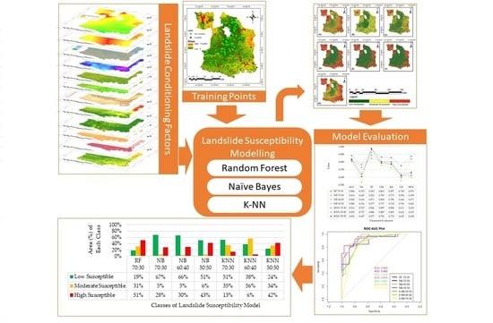
2. Materials and Methods
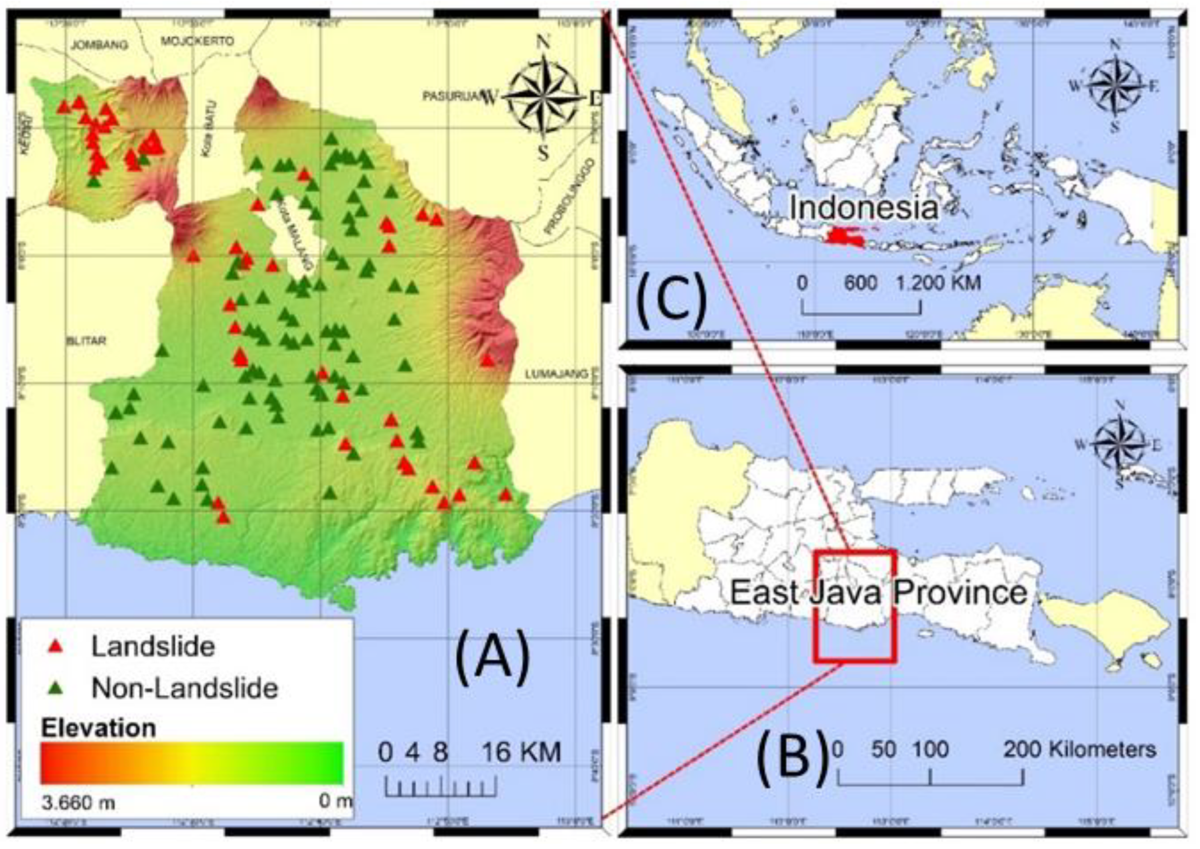
2.1. Study Area
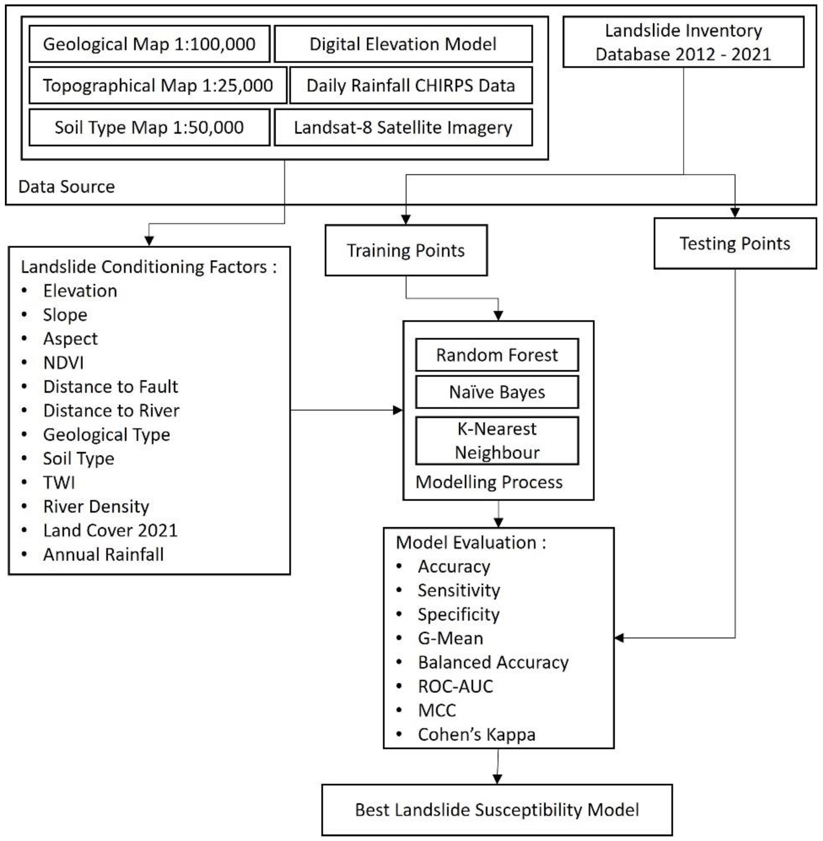
2.2. Data Sources
2.2.1. Data Training Sample
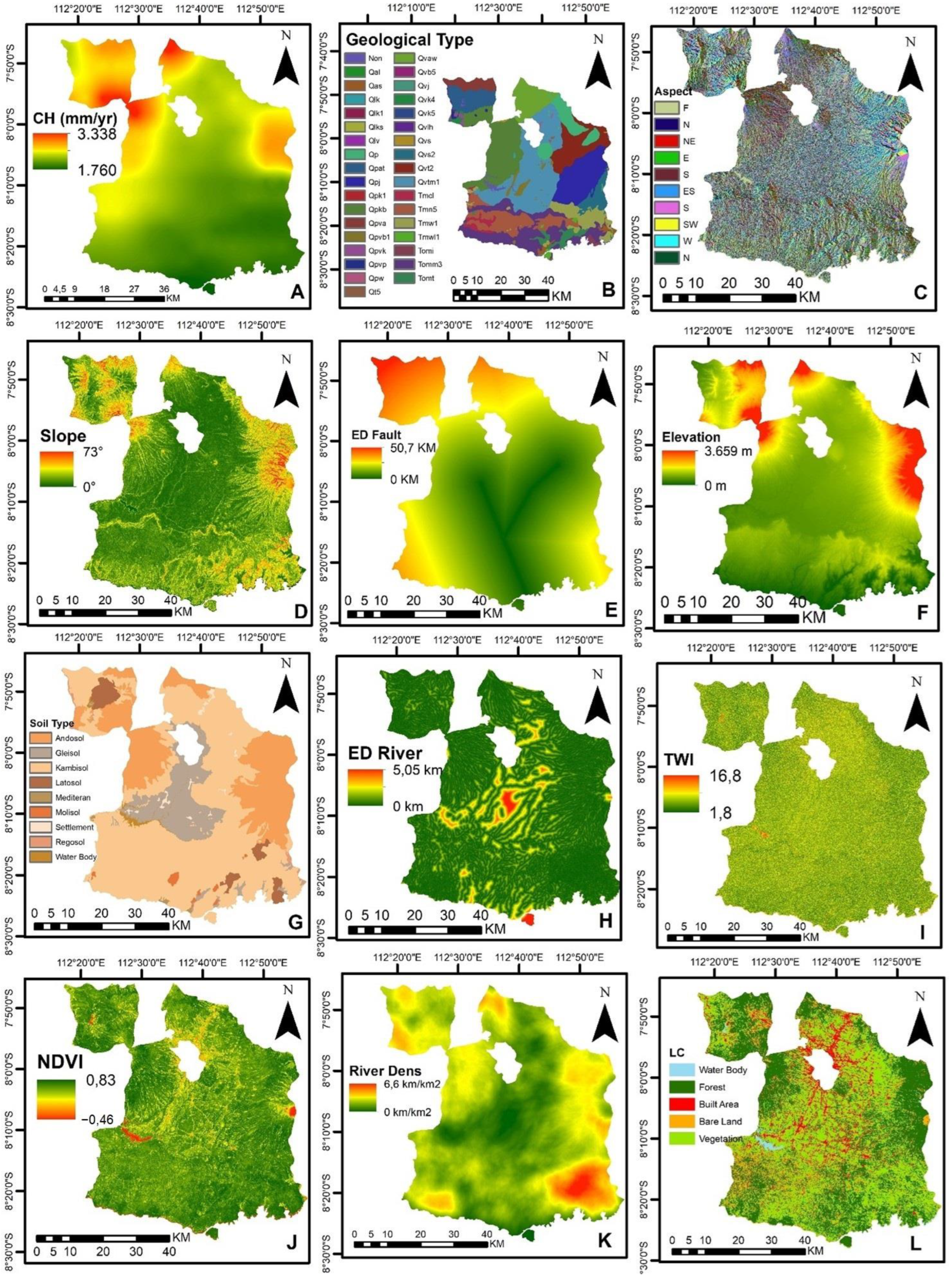
2.2.2. Spatial Data Landslide Conditioning Factors
Elevation Data
Geological Map Data
Soil Type Data
Landsat-8 OLI TIRS Imagery Data
Annual Rainfall Data
River Net Data
2.3. Methods
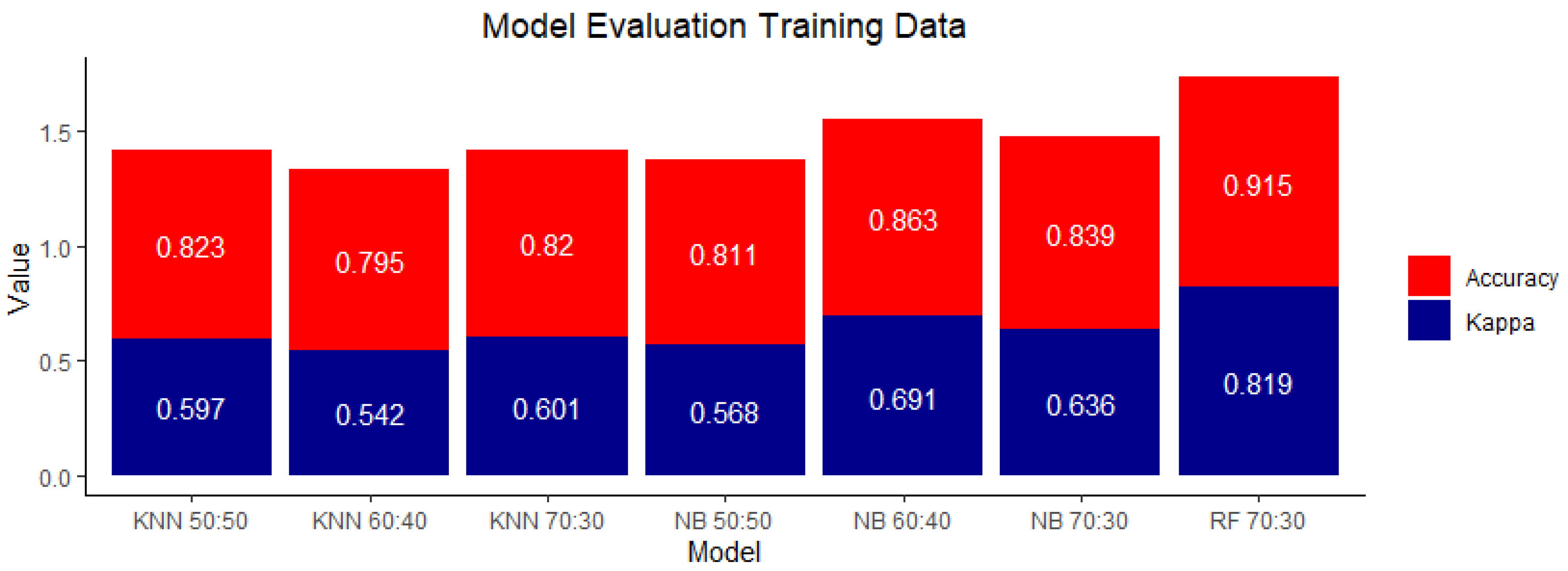
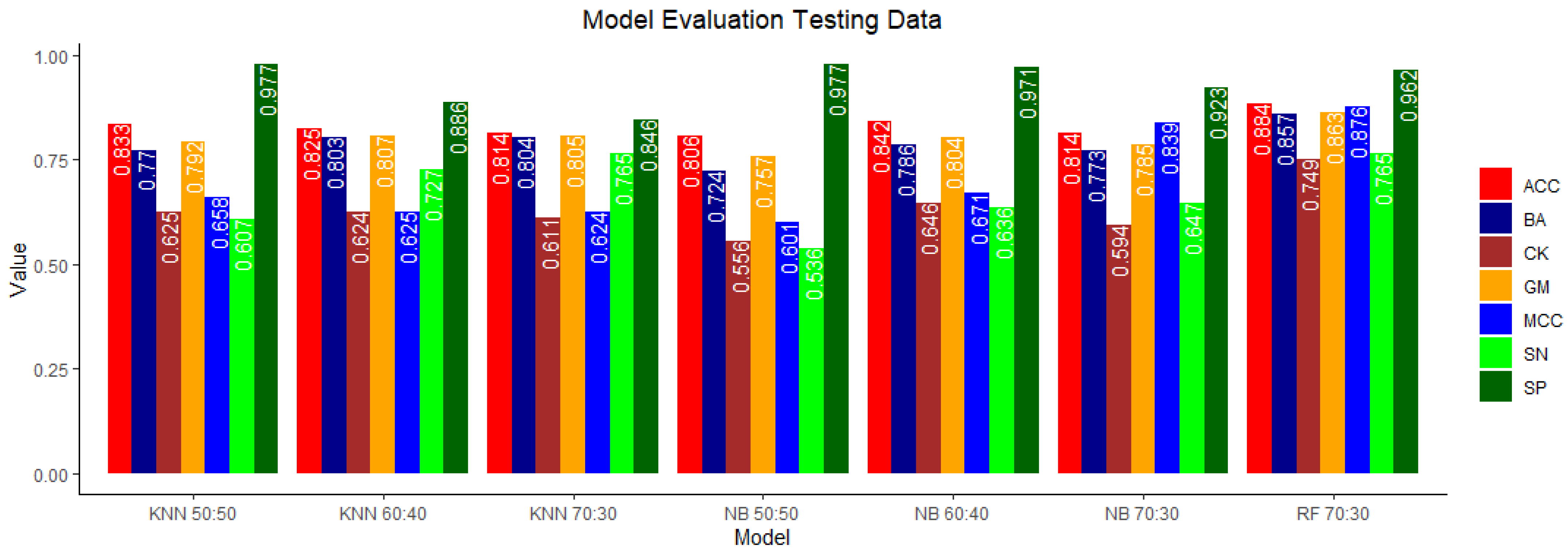
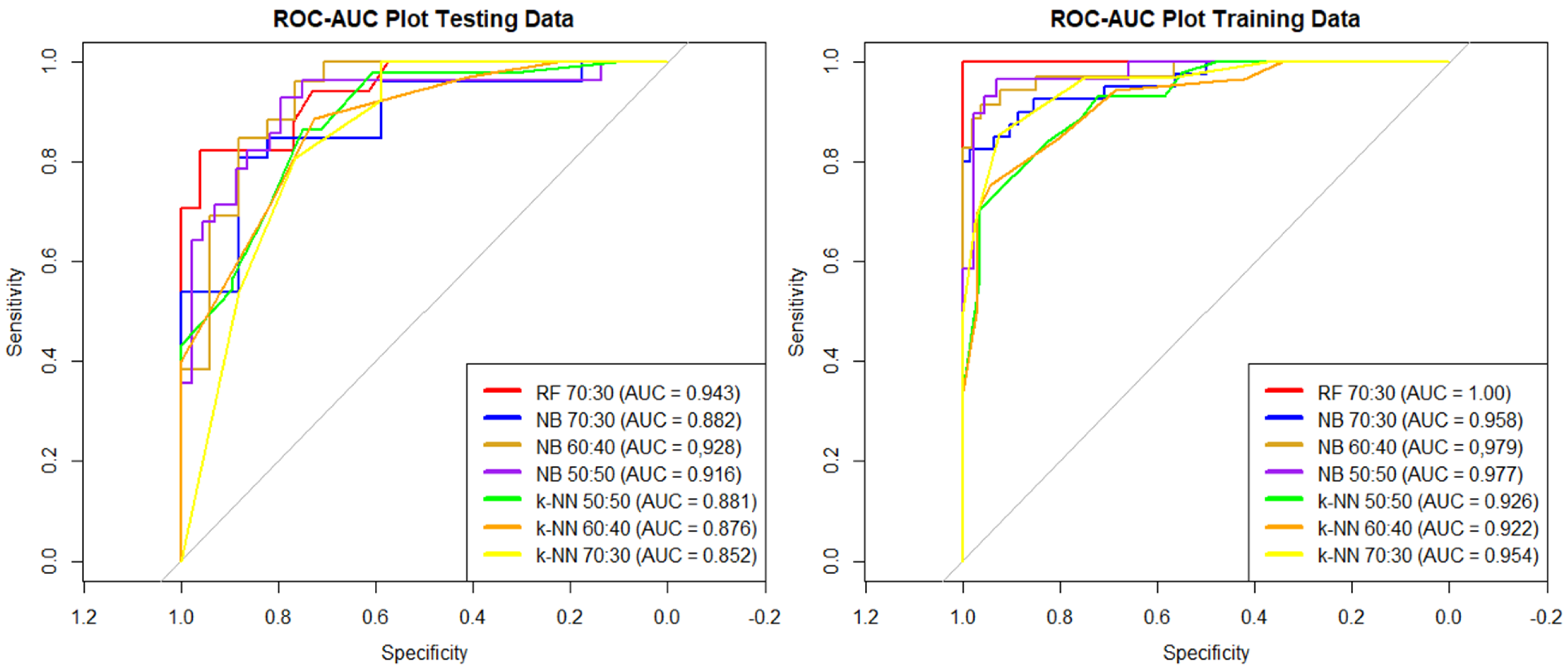
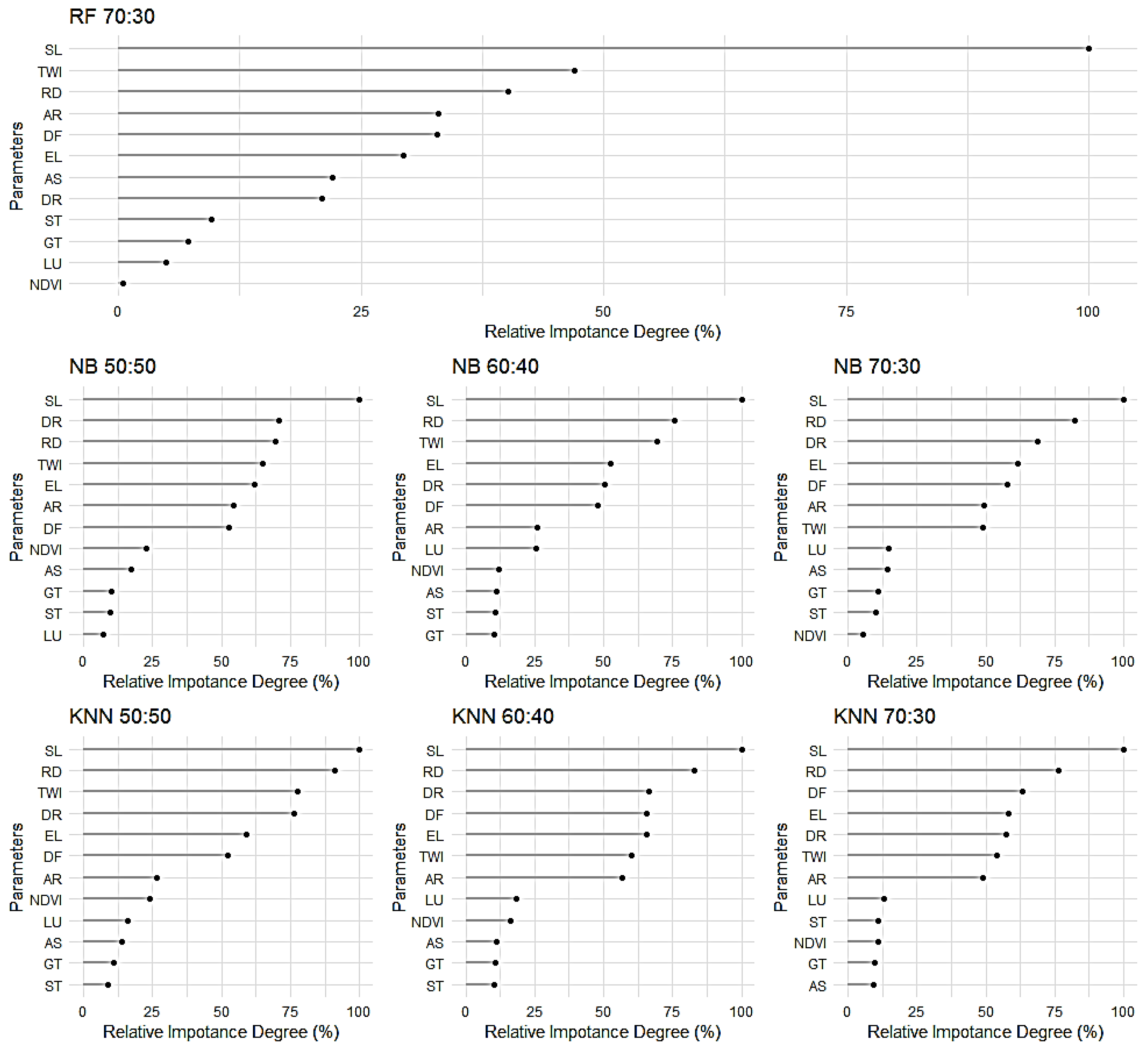
3. Results
3.1. Continuous Data Parameter Normality Characteristics
3.2. Landslide Susceptibility Modeling Results
4. Discussion
5. Conclusions
Author Contributions
Funding
Data Availability Statement
Acknowledgments
Conflicts of Interest
References
- Skempton, A.W.; Hutchinson, J. Stability of natural slopes and embankment foundations. In Proceedings of the 7th International Conference on Soil Mechanics and Foundation Engineering, Mexico City, Mexico, 29 August 1969; pp. 291–340. [Google Scholar]
- Muntohar, A. Tanah Longsor: Analisis-Prediksi-Mitigasi, 1st ed.; Universitas Muhammadiyah Yogyakarta: Kasihan, Indonesia, 2012. [Google Scholar]
- Keefer, D.K. Investigating landslides caused by earthquakes—A historical review. Surv. Geophys. 2002, 23, 473–510. [Google Scholar] [CrossRef]
- Lu, P.; Bai, S.; Casagli, N. Investigating spatial patterns of persistent scatterer interferometry point targets and landslide occurrences in the Arno River basin. Remote Sens. 2014, 6, 6817–6843. [Google Scholar] [CrossRef]
- Hong, H.; Naghibi, S.A.; Pourghasemi, H.R.; Pradhan, B. GIS-based landslide spatial modeling in Ganzhou City, China. Arab. J. Geosci. 2016, 9, 1–26. [Google Scholar] [CrossRef]
- El Naqa, I.; Murphy, M.J. What is machine learning? In Machine Learning in Radiation Oncology; Springer: Berlin/Heidelberg, Germany, 2015; pp. 3–11. [Google Scholar]
- Ahmad Hania, A. Mengenal Artificial Intelligence, Machine Learning, & Deep Learning. Available online: https://amt-it.com/mengenal-perbedaan-artificial-inteligence-machine-learning-deep-learning/ (accessed on 3 July 2022).
- Youssef, A.M.; Pourghasemi, H.R. Landslide susceptibility mapping using machine learning algorithms and comparison of their performance at Abha Basin, Asir Region, Saudi Arabia. Geosci. Front. 2021, 12, 639–655. [Google Scholar] [CrossRef]
- Yanbin, M.; Hongrui, L.; Lin, W.; Wengang, Z.; Zhengwei, Z.; Haiqing, Y.; Luqi, W.; Xingzhong, Y. Machine learning algorithms and techniques for landslide susceptibility investigation: A literature review. J. Civ. Environ. Eng. 2022, 44, 53–67. [Google Scholar]
- He, Q.; Shahabi, H.; Shirzadi, A.; Li, S.; Chen, W.; Wang, N.; Chai, H.; Bian, H.; Ma, J.; Chen, Y.; et al. Landslide spatial modelling using novel bivariate statistical based Naïve Bayes, RBF Classifier, and RBF Network machine learning algorithms. Sci. Total Environ. 2019, 663, 1–15. [Google Scholar] [CrossRef] [PubMed]
- Al-Najjar, H.A.H.; Pradhan, B. Spatial landslide susceptibility assessment using machine learning techniques assisted by additional data created with generative adversarial networks. Geosci. Front. 2021, 12, 625–637. [Google Scholar] [CrossRef]
- Abraham, M.T.; Satyam, N.; Lokesh, R.; Pradhan, B.; Alamri, A. Factors Affecting Landslide Susceptibility Mapping: Assessing the Influence of Different Machine Learning Approaches, Sampling Strategies and Data Splitting. Land 2021, 10, 989. [Google Scholar] [CrossRef]
- Adab, H.; Atabati, A.; Oliveira, S.; Moghaddam Gheshlagh, A. Assessing fire hazard potential and its main drivers in Mazandaran province, Iran: A data-driven approach. Environ. Monit. Assess. 2018, 190, 670. [Google Scholar] [CrossRef]
- Lin, J.; He, P.; Yang, L.; He, X.; Lu, S.; Liu, D. Predicting future urban waterlogging-prone areas by coupling the maximum entropy and FLUS model. Sustain. Cities Soc. 2022, 80, 103812. [Google Scholar] [CrossRef]
- Rahmati, O.; Golkarian, A.; Biggs, T.; Keesstra, S.; Mohammadi, F.; Daliakopoulos, I.N. Land subsidence hazard modeling: Machine learning to identify predictors and the role of human activities. J. Environ. Manage 2019, 236, 466–480. [Google Scholar] [CrossRef]
- Shahzad, N.; Ding, X.; Abbas, S. A Comparative Assessment of Machine Learning Models for Landslide Susceptibility Mapping in the Rugged Terrain of Northern Pakistan. Appl. Sci. 2022, 12, 2280. [Google Scholar] [CrossRef]
- Laila Nugraha, A.; Sukmono, A.; Sugistu Firdau, H.S.; Lestari, S. Study of Accuracy in Landslide Mapping Assessment Using GIS and AHP, A Case Study of Semarang Regency. KnE Eng. 2019. [Google Scholar] [CrossRef]
- Bachri, S.; Sumarmi; Yudha Irawan, L.; Utaya, S.; Dwitri Nurdiansyah, F.; Erfika Nurjanah, A.; Wahyu Ning Tyas, L.; Amri Adillah, A.; Setia Purnama, D. Landslide Susceptibility Mapping (LSM) in Kelud Volcano Using Spatial Multi-Criteria Evaluation. IOP Conf. Ser. Earth Environ. Sci. 2019, 273, 012014. [Google Scholar] [CrossRef]
- Bachri, S.; Shrestha, R.P.; Yulianto, F.; Sumarmi, S.; Utomo, K.S.B.; Aldianto, Y.E. Mapping landform and landslide susceptibility using remote sensing, gis and field observation in the southern cross road, Malang regency, East Java, Indonesia. Geosciences 2021, 11, 4. [Google Scholar] [CrossRef]
- Ghasemian, B.; Shahabi, H.; Shirzadi, A.; Al-Ansari, N.; Jaafari, A.; Kress, V.R.; Geertsema, M.; Renoud, S.; Ahmad, A. A Robust Deep-Learning Model for Landslide Susceptibility Mapping: A Case Study of Kurdistan Province, Iran. Sensors 2022, 22, 1573. [Google Scholar] [CrossRef]
- Pham, B.T.; Vu, V.D.; Costache, R.; Van Phong, T.; Ngo, T.Q.; Tran, T.-H.; Nguyen, H.D.; Amiri, M.; Tan, M.T.; Trinh, P.T.; et al. Landslide susceptibility mapping using state-of-the-art machine learning ensembles. Geocarto Int. 2022, 37, 5175–5200. [Google Scholar] [CrossRef]
- Darminto, M.R.; Widodob, A.; Alfatinahc, A.; Chuc, H.-J. High-Resolution Landslide Susceptibility Map Generation using Machine Learning (Case Study in Pacitan, Indonesia). Int. J. Adv. Sci. Eng. Inf. Technol. 2021, 11, 369–379. [Google Scholar] [CrossRef]
- Tsangaratos, P.; Ilia, I. Comparison of a logistic regression and Naïve Bayes classifier in landslide susceptibility assessments: The influence of models complexity and training dataset size. Catena 2016, 145, 164–179. [Google Scholar] [CrossRef]
- Xu, C.; Dai, F.; Xu, X.; Lee, Y.H. GIS-based support vector machine modeling of earthquake-triggered landslide susceptibility in the Jianjiang River watershed, China. Geomorphology 2012, 145–146, 70–80. [Google Scholar] [CrossRef]
- Vakhshoori, V.; Pourghasemi, H.R.; Zare, M.; Blaschke, T. Landslide susceptibility mapping using GIS-based data mining algorithms. Water 2019, 11, 2292. [Google Scholar] [CrossRef]
- Tseng, C.M.; Lin, C.W.; Hsieh, W.D. Landslide susceptibility analysis by means of event-based multi-temporal landslide inventories. Nat. Hazards Earth Syst. Sci. Discuss. 2015, 3, 1137–1173. [Google Scholar]
- Iswari, M.Y.; Anggraini, K. Demnas: Model Digital Ketinggian Nasional Untuk Aplikasi Kepesisiran. Oseana 2018, 43. [Google Scholar] [CrossRef]
- Ronodirdjo, M.Z. Buku Ajar Pengantar Geologi; Duta Pustaka Ilmu: Mataram, Indonesia, 2019. [Google Scholar]
- Varianti, E. Geologi daerah Sumberbening dan sekitarnya Kecamatan Bantur Kabupaten Malang Provinsi Jawa Timur. J. Online Mhs. Bid. Tek. Geol. 2019, 1, 1–10. [Google Scholar]
- Wasis, W.; Sunaryo, S.; Susilo, A. Local Fault Line Tracing in Sri Mulyo Village, Dampit Sub District, Malang Regency Based on Geophysical Data. Nat. B J. Health Environ. Sci. 2011, 1, 41–50. [Google Scholar]
- Islami, D.A.L. Al Geologi daerah Klepu dan sekitarnya, Kecamatan Sumbermanjing Wetan Kabupaten Malang, Provinsi Jawa Timur. J. Online Mhs. Bid. Tek. Geol. 2017, 1, 1–12. [Google Scholar]
- Martins, K.G.; Marques, M.C.M.; dos Santos, E.; Marques, R. Effects of soil conditions on the diversity of tropical forests across a successional gradient. For. Ecol. Manag. 2015, 349, 4–11. [Google Scholar] [CrossRef]
- Viet, L.D.; Chi, C.N.; Tien, C.N.; Quoc, D.N. The Effect of the Normalized Difference Vegetation Index to Landslide Susceptibility using Optical Imagery Sentinel 2 and Landsat 8. In Proceedings of the 4th Asia Pacific Meeting on Near Surface Geoscience & Engineering, Online, 30 November–2 December 2021; Volume 2021, pp. 1–5. [Google Scholar]
- Yang, I.; Acharya, T.D. Exploring Landsat 8. Available online: https://www.researchgate.net/profile/Tri-Acharya/publication/311901147_Exploring_Landsat_8/links/589c0de6458515e5f4549e58/Exploring-Landsat-8.pdf%0Ahttp://earthobservatory.nasa.gov/IOTD/ (accessed on 20 April 2022).
- Gessesse, A.A.; Melesse, A.M. Chapter 8—Temporal relationships between time series CHIRPS-rainfall estimation and eMODIS-NDVI satellite images in Amhara Region, Ethiopia. In Extreme Hydrology and Climate Variability; Melesse, A.M., Abtew, W., Senay, G.B.T.-E.H., Eds.; Elsevier: Amsterdam, The Netherlands, 2019; pp. 81–92. ISBN 978-0-12-815998-9. [Google Scholar]
- Pettorelli, N. The Normalized Difference Vegetation Index; Oxford University Press: Oxford, UK, 2013; ISBN 0199693161. [Google Scholar]
- Hashim, H.; Abd Latif, Z.; Adnan, N.A. Urban vegetation classification with ndvi threshold value method with very high resolution (vhr) pleiades imagery. Int. Arch. Photogramm. Remote Sens. Spat. Inf. Sci.-ISPRS Arch. 2019, 42, 237–240. [Google Scholar] [CrossRef]
- Funk, C.C.; Peterson, P.J.; Landsfeld, M.F.; Pedreros, D.H.; Verdin, J.P.; Rowland, J.D.; Romero, B.E.; Husak, G.J.; Michaelsen, J.C.; Verdin, A.P. A quasi-global precipitation time series for drought monitoring. US Geol. Surv. Data Ser. 2014, 832, 1–12. [Google Scholar]
- Breiman, L. Random forests. Mach. Learn. 2001, 45, 5–32. [Google Scholar] [CrossRef]
- Liaw, A.; Wiener, M. Classification and regression by randomForest. R News 2002, 2, 18–22. [Google Scholar]
- Rodriguez-Galiano, V.F.; Ghimire, B.; Rogan, J.; Chica-Olmo, M.; Rigol-Sanchez, J.P. An assessment of the effectiveness of a random forest classifier for land-cover classification. ISPRS J. Photogramm. Remote Sens. 2012, 67, 93–104. [Google Scholar] [CrossRef]
- Cunningham, P.; Delany, S.J. K-Nearest Neighbour Classifiers-A Tutorial. ACM Comput. Surv. 2021, 54, 1–25. [Google Scholar] [CrossRef]
- Gonçalves, D.N.S.; Gonçalves, C.D.M.; De Assis, T.F.; Silva, M.A. Da Analysis of the difference between the euclidean distance and the actual road distance in Brazil. Transp. Res. Procedia 2014, 3, 876–885. [Google Scholar] [CrossRef]
- Vikramkumar, B.V. Trilochan Bayes and Naive Bayes Classifier. arXiv 2014, arXiv:1404.0933. [Google Scholar]
- Zhang, H. The optimality of Naive Bayes. In Proceedings of the Seventeenth International Florida Artificial Intelligence Research Society Conference, Sarasota, FL, USA, 12–14 May 2004; Volume 2, pp. 562–567. [Google Scholar]
- Kurniawan, D. Pengenalan Machine Learning dengan Python; PT Elex Media Komputindo: Jakarta, Indonesia, 2020. [Google Scholar]
- Akinci, H.; Kilicoglu, C. Random Forest-Based Landslide Susceptibility Mapping in Coastal Regions of Artvin, Turkey. ISPRS Int. J. Geo-Inf. 2020, 9, 553. [Google Scholar] [CrossRef]
- Li, X.; Cheng, J.; Yu, D.; Han, Y. Research on Non-Landslide Selection Method for Landslide Hazard Mapping. Res. Sq. 2021, 1–11. [Google Scholar]
- Hossin, M.; Sulaiman, M.N. A Review on Evaluation Metrics for Data Classification Evaluations. Int. J. Data Min. Knowl. Manag. Process 2015, 5, 1–11. [Google Scholar] [CrossRef]
- Zhang, H.; Song, Y.; Xu, S.; He, Y.; Li, Z.; Yu, X.; Liang, Y.; Wu, W.; Wang, Y. Combining a class-weighted algorithm and machine learning models in landslide susceptibility mapping: A case study of Wanzhou section of the Three Gorges Reservoir, China. Comput. Geosci. 2022, 158, 104966. [Google Scholar] [CrossRef]
- Chicco, D.; Warrens, M.J.; Jurman, G. The Matthews correlation coefficient (MCC) is more informative than Cohen’s Kappa and Brier score in binary classification assessment. IEEE Access 2021, 9, 78368–78381. [Google Scholar] [CrossRef]
- Aslam, M. Introducing Kolmogorov-Smirnov Tests under Uncertainty: An Application to Radioactive Data. ACS Omega 2020, 5, 914–917. [Google Scholar] [CrossRef]
- Massey Jr, F.J. The Kolmogorov-Smirnov test for goodness of fit. J. Am. Stat. Assoc. 1951, 46, 68–78. [Google Scholar] [CrossRef]
- Fleming, T.R.; O’Fallon, J.R.; O’Brien, P.C.; Harrington, D.P. Modified Kolmogorov-Smirnov test procedures with application to arbitrarily right-censored data. Biometrics 1980, 36, 607–625. [Google Scholar] [CrossRef]
- Lee, S.; Choi, J.; Min, K. Landslide susceptibility analysis and verification using the Bayesian probability model. Environ. Geol. 2002, 43, 120–131. [Google Scholar] [CrossRef]
- Hussain, M.A.; Chen, Z.; Zheng, Y.; Shoaib, M.; Shah, S.U.; Ali, N.; Afzal, Z. Landslide Susceptibility Mapping Using Machine Learning Algorithm Validated by Persistent Scatterer In-SAR Technique. Sensors 2022, 22, 3119. [Google Scholar] [CrossRef] [PubMed]
- Bui, D.T.; Tsangaratos, P.; Nguyen, V.T.; Van Liem, N.; Trinh, P.T. Comparing the prediction performance of a Deep Learning Neural Network model with conventional machine learning models in landslide susceptibility assessment. Catena 2020, 188, 104426. [Google Scholar] [CrossRef]
- Abu El-Magd, S.A.; Ali, S.A.; Pham, Q.B. Spatial modeling and susceptibility zonation of landslides using random forest, naïve bayes and K-nearest neighbor in a complicated terrain. Earth Sci. Inform. 2021, 14, 1227–1243. [Google Scholar] [CrossRef]
- Park, S.-J.; Lee, D.-K. Predicting susceptibility to landslides under climate change impacts in metropolitan areas of South Korea using machine learning. Geomat. Nat. Hazards Risk 2021, 12, 2462–2476. [Google Scholar] [CrossRef]
- Soria, D.; Garibaldi, J.M.; Ambrogi, F.; Biganzoli, E.M.; Ellis, I.O. A ‘non-parametric’ version of the naive Bayes classifier. Knowl.-Based Syst. 2011, 24, 775–784. [Google Scholar] [CrossRef]
- Marjanović, M.; Kovačević, M.; Bajat, B.; Voženílek, V. Landslide susceptibility assessment using SVM machine learning algorithm. Eng. Geol. 2011, 123, 225–234. [Google Scholar] [CrossRef]
- Merghadi, A.; Yunus, A.P.; Dou, J.; Whiteley, J.; ThaiPham, B.; Bui, D.T.; Avtar, R.; Abderrahmane, B. Machine learning methods for landslide susceptibility studies: A comparative overview of algorithm performance. Earth-Sci. Rev. 2020, 207, 103225. [Google Scholar] [CrossRef]
- Nakileza, B.R.; Nedala, S. Topographic influence on landslides characteristics and implication for risk management in upper Manafwa catchment, Mt Elgon Uganda. Geoenviron. Disasters 2020, 7, 1–13. [Google Scholar] [CrossRef]
- Dai, F.C.; Lee, C.F.; Li, J.; Xu, Z.W. Assessment of landslide susceptibility on the natural terrain of Lantau Island, Hong Kong. Environ. Geol. 2001, 40, 381–391. [Google Scholar] [CrossRef]
- Nourani, V.; Pradhan, B.; Ghaffari, H.; Sharifi, S.S. Landslide susceptibility mapping at Zonouz Plain, Iran using genetic programming and comparison with frequency ratio, logistic regression, and artificial neural network models. Nat. Hazards 2014, 71, 523–547. [Google Scholar] [CrossRef]
- Çellek, S. Effect of the slope angle and its classification on landslides. Himal. Geol. 2022, 43, 85–95. [Google Scholar]
- Christian, J.T.; Baecher, G.B. DW Taylor and the foundations of modern soil mechanics. J. Geotech. Geoenviron. Eng. 2015, 141, 2514001. [Google Scholar] [CrossRef]
- Take, W.A.; Bolton, M.D.; Wong, P.C.P.; Yeung, F.J. Evaluation of landslide triggering mechanisms in model fill slopes. Landslides 2004, 1, 173–184. [Google Scholar] [CrossRef]
- Kim, J.-C.; Lee, S.; Jung, H.-S.; Lee, S. Landslide susceptibility mapping using random forest and boosted tree models in Pyeong-Chang, Korea. Geocarto Int. 2018, 33, 1000–1015. [Google Scholar] [CrossRef]
- Gonzalez-Ollauri, A.; Mickovski, S.B. Hydrological effect of vegetation against rainfall-induced landslides. J. Hydrol. 2017, 549, 374–387. [Google Scholar] [CrossRef]
- Norris, J.E.; Stokes, A.; Mickovski, S.B.; Cammeraat, E.; Van Beek, R.; Nicoll, B.C.; Achim, A. Slope Stability and Erosion Control: Ecotechnological Solutions; Springer Science & Business Media: Berlin/Heidelberg, Germany, 2008; ISBN 1402066767. [Google Scholar]
- Guillard, C.; Zezere, J. Landslide Susceptibility Assessment and Validation in the Framework of Municipal Planning in Portugal: The Case of Loures Municipality. Environ. Manag. 2012, 50, 721–735. [Google Scholar] [CrossRef]
- Karsli, F.; Atasoy, M.; Yalcin, A.; Reis, S.; Demir, O.; Gokceoglu, C. Effects of land-use changes on landslides in a landslide-prone area (Ardesen, Rize, NE Turkey). Environ. Monit. Assess. 2009, 156, 241–255. [Google Scholar] [CrossRef]
- Tufaila, M.; Alam, S. Karakteristik tanah dan evaluasi lahan untuk pengembangan tanaman padi sawah di kecamatan oheo kabupaten konawe utara. Agriplus 2014, 24, 184–194. [Google Scholar]
- Balai, B. Ksda Faktor Penyebab Tanah Longsor. Available online: http://ksdasulsel.menlhk.go.id/post/faktor-penyebab-tanah-longsor#:~:text=Tanahyangkurangpadatdan,longsor%2Cterutamabilaterjadihujan (accessed on 3 July 2022).
- Mahmood, K.; Kim, J.M.; Ashraf, M. The effect of soil type on matric suction and stability of unsaturated slope under uniform rainfall. KSCE J. Civ. Eng. 2016, 20, 1294–1299. [Google Scholar] [CrossRef]
- Yeh, H.-F.; Lee, C.-C.; Lee, C.-H. A rainfall-infiltration model for unsaturated soil slope stability. Sustain. Environ. Res. 2008, 18, 271–278. [Google Scholar]
- Igwe, O. The geotechnical characteristics of landslides on the sedimentary and metamorphic terrains of South-East Nigeria, West Africa. Geoenviron. Disasters 2015, 2, 1–14. [Google Scholar] [CrossRef]
- Di, B.; Stamatopoulos, C.A.; Stamatopoulos, A.C.; Liu, E.; Balla, L. Proposal, application and partial validation of a simplified expression evaluating the stability of sandy slopes under rainfall conditions. Geomorphology 2021, 395, 107966. [Google Scholar] [CrossRef]
- Chen, W.; Xie, X.; Peng, J.; Wang, J.; Duan, Z.; Hong, H. GIS-based landslide susceptibility modelling: A comparative assessment of kernel logistic regression, Naïve-Bayes tree, and alternating decision tree models. Geomat. Nat. Hazards Risk 2017, 8, 950–973. [Google Scholar] [CrossRef]
- Gilliam, F.S.; Hédl, R.; Chudomelová, M.; McCulley, R.L.; Nelson, J.A. Variation in vegetation and microbial linkages with slope aspect in a montane temperate hardwood forest. Ecosphere 2014, 5, 1–17. [Google Scholar] [CrossRef]
- Singh, S. Understanding the Role of Slope Aspect in Shaping the Vegetation Attributes and Soil Properties in Montane Ecosystems. Available online: www.tropecol.com (accessed on 4 April 2022).
- van Westen, C. Landslide Risk Assessments for Decision-Making. In Proceedings of the 2012 UR Forum, Cape Town, South Africa, 2–6 July 2012; pp. 67–71. [Google Scholar]


| Code | Formation | Rock Formation | Deposit | Area (km2) |
|---|---|---|---|---|
| Qvtm1 | Malang tuff | E: I: PA | Volcanism: subaerial—Volcanism | 633.995 |
| Qpkb | Kawi-butak volcanic rock | E: I: PC | Volcanism: subaerial—Volcanism | 446.265 |
| Tomm3 | Mandalika formation | E: I: L | Volcanism: subaerial—Volcanism | 401.839 |
| Qpj | Jombang formation | ST: CC: CE: B | Volcanism: subaerial—Volcanism: | 331.369 |
| Tmn5 | Nampol formation | ST: CC: M: S | Sedimentation: transitional—Sed | 277.764 |
| Qvt2 | Tengger volcanic rock | E: I: PA | Volcanism: subaerial—Volcanism | 238.221 |
| Qvaw | Arjuna-Welirang volcanic rock | E: I: PC | Volcanism: subaerial—Volcanism | 184.673 |
| Tmw1 | Wuni formation | ST: CC: CE: B | — | 184.217 |
| Qp | Western volcanic rock | E: I: PC | Volcanism: subaerial—Volcanism | 171.113 |
| Qpat | Anjasmara old volcanic rock | E: I: PC | Volcanism: subaerial—Volcanism | 160.352 |
| Qvs2 | Semeru volcanic deposit | E: I: L | Volcanism: subaerial—Volcanism | 96.447 |
| Qpva | Anjasmara young volcano | E: I: PC | Volcanism: subaerial—Volcanism | 87.365 |
| Tomt | Tuff member | E: I: PA | Volcanism: subaerial—Volcanism | 70.339 |
| Tmcl | Campurdarat formation | ST: CC: LS | Sedimentation: littoral—Sedimen | 45.227 |
| Qpvb1 | Buring volcanic deposit | E: MC: L | Volcanism: subaerial—Volcanism | 39.199 |
| Qas | Swamp and river deposits | S: CC: M: S | Sedimentation: terrestrial: fluv | 26.346 |
| Non | Lake | - | - | 20.240 |
| Tmwl1 | Wonosari formation | ST: R: LS | Sedimentation: littoral: reef—S | 15.264 |
| Qvk4 | Kelud young volcano | E: I: PC | Volcanism: subaerial—Volcanism: | 13.200 |
| Qpvk | Kelud old volcanic rock | E: I: L | Volcanism: subaerial—Volcanism | 11.789 |
| Tomi | Rock intrusion | IE: I | Plutonism: sub-volcanic—Plutoni | 11.564 |
| Qpvp | Marikeng volcanic rock | IE: I | Plutonism: sub-volcanic—Plutoni | 6.937 |
| Qvlh | Lava deposit | E: I: PC | Volcanism: subaerial—Volcanism | 5.602 |
| Qvs | Tengger volcanic sand | E: I: PA | Volcanism: subaerial—Volcanism | 4.173 |
| Qvk5 | Kepolo volcanic deposit | E: I: L | Volcanism: subaerial—Volcanism | 3.084 |
| Qpw | Welang formation | ST: CC: M: S | Sedimentation: terrestrial: allu | 2.546 |
| Qvj | Jembangan volcanic deposit | E: MC: L | Volcanism: subaerial—Volcanism | 2.225 |
| Qt5 | Terrace deposit | ST: CC: A | Sedimentation: terrestrial: allu | 2.179 |
| Qlk | Katu’s peak lava | E: I: L | Volcanism: subaerial—Volcanism | 1.829 |
| Qal | Aluvial and coastal deposit | ST: CC: A | Sedimentation: terrestrial: fluv | 1.130 |
| Qvb5 | Bromo volcanic rock | E: I: PC | Volcanism: subaerial—Volcanism: | 0.810 |
| Qlks | Lava Parasite Kepolo Mt. Semeru | E: I: L | Volcanism: subaerial—Volcanism | 0.727 |
| Qlk1 | Lava andesit parasit | E: I: L | Volcanism: subaerial—Volcanism | 0.058 |
| Qlv | Avalanche deposits from volcanoes | E: I: PC | Volcanism: subaerial—Volcanism | 0.035 |
| Qpk1 | Kalipucang formation | ST: CC: CE: CL | Sedimentation: terrestrial: fluv | 0.001 |
| Metric | Equation | Objective |
|---|---|---|
| ACC | Indicates the ratio of correct prediction to the total number of evaluation samples [49]. | |
| SN | Measures the fraction of correctly classified positive patterns [49]. | |
| SP | Measures the fraction of correctly classified negative patterns [49]. | |
| GM | Measures the average sensitivity (sn) obtained under each class [50]. | |
| BA | Measures the roots of the products sn and sp [50]. | |
| CK | Consistency value between 2 raters (observation and prediction) [51]. | |
| MCC | Measures the performance of the classification algorithm through the correlation between observations and predictions [51]. | |
| ROC-AUC | The ROC curve is built based on sn (sb-Y) with sp (sb-X), and AUC is an integral ROC [10]. |
| Parameter | Landslide Training Point | Non-Landslide Training Point | ||||
|---|---|---|---|---|---|---|
| D-Value | p-Value | Normal Distribution | D-Value | p-Value | Normal Distribution | |
| River Density | 0.167 | 2.32 × 10⁻⁶ | No | 0.096 | 0.04519 | No |
| Annual Rainfall | 0.165 | 3.47 × 10⁻⁶ | No | 0.104 | 0.01946 | No |
| Distance to Fault | 0.258 | 6.76 × 10⁻¹⁶ | No | 0.151 | 3.92 × 10⁻⁵ | No |
| Elevation | 0.107 | 0.01467 | No | 0.101 | 0.02766 | No |
| Distance to River | 0.192 | 5.39 × 10⁻⁷ | No | 0.152 | 3.03 × 10⁻⁵ | No |
| NDVI | 0.175 | 5.39 × 10⁻⁷ | No | 0.149 | 4.74 × 10⁻⁵ | No |
| Slope | 0.140 | 2.04 × 10⁻⁴ | No | 0.113 | 7.78 × 10⁻³ | No |
| TWI | 0.088 | 9.00 × 10⁻² | Yes | 0.205 | 8.66 × 10⁻¹⁰ | No |
Publisher’s Note: MDPI stays neutral with regard to jurisdictional claims in published maps and institutional affiliations. |
© 2022 by the authors. Licensee MDPI, Basel, Switzerland. This article is an open access article distributed under the terms and conditions of the Creative Commons Attribution (CC BY) license (https://creativecommons.org/licenses/by/4.0/).
Share and Cite
Nurwatik, N.; Ummah, M.H.; Cahyono, A.B.; Darminto, M.R.; Hong, J.-H. A Comparison Study of Landslide Susceptibility Spatial Modeling Using Machine Learning. ISPRS Int. J. Geo-Inf. 2022, 11, 602. https://doi.org/10.3390/ijgi11120602
Nurwatik N, Ummah MH, Cahyono AB, Darminto MR, Hong J-H. A Comparison Study of Landslide Susceptibility Spatial Modeling Using Machine Learning. ISPRS International Journal of Geo-Information. 2022; 11(12):602. https://doi.org/10.3390/ijgi11120602
Chicago/Turabian StyleNurwatik, Nurwatik, Muhammad Hidayatul Ummah, Agung Budi Cahyono, Mohammad Rohmaneo Darminto, and Jung-Hong Hong. 2022. "A Comparison Study of Landslide Susceptibility Spatial Modeling Using Machine Learning" ISPRS International Journal of Geo-Information 11, no. 12: 602. https://doi.org/10.3390/ijgi11120602
APA StyleNurwatik, N., Ummah, M. H., Cahyono, A. B., Darminto, M. R., & Hong, J.-H. (2022). A Comparison Study of Landslide Susceptibility Spatial Modeling Using Machine Learning. ISPRS International Journal of Geo-Information, 11(12), 602. https://doi.org/10.3390/ijgi11120602