Evaluating Stable Matching Methods and Ridesharing Techniques in Optimizing Passenger Transportation Cost and Companionship

Abstract

In this work, we propose a Game Theory-based pricing solution to the ridesharing problem of taxi commuters that addresses the optimal selection of their travel companionship and effectively minimizes their cost. Two stable matching techniques are proposed in this study, namely: First-Come, First-Served (FCFS) and Best Time Sharing (BT). FCFS discovers pairs based on earliest time of pair occurrences, while BT prioritizes selecting pairs with high proportion of shared distance between passengers to the overall distance of their trips. We evaluate our methods through extensive simulations from empirical taxi trajectories from Jakarta, Singapore, and New York. Results in terms of post-stable matching, cost savings, successful matches, and total number of trips have been evaluated to gauge the performance with respect to the no ridesharing condition. BT outperformed FCFS in terms of generating more pairs with compatible routes. Additionally, in the New York dataset with high amount of trip density, BT has efficiently reduced the number of trips present at a given time. On the other hand, FCFS has been more effective in pairing trips for the Jakarta and Singapore datasets because of lower density due to limited number of trajectories. The Game Theory (GT) pricing model proved to generally be the most beneficial to the ride share’s cost savings, specifically leaning toward the passenger benefits. Analysis has shown that the stable matching algorithm reduced the overall number of trips while still adhering to the temporal frequency of trips within the dataset. Moreover, our developed Best Time Pairing and Game Theory Pricing methods served the most efficient based on passenger cost savings. Applying these stable matching algorithms will benefit more users and will encourage more ridesharing instances.

1. Introduction

The continuous improvement of mobile internet technologies has prompted a multitude of opportunities for people to interact, share, and avail resources in real-time over the internet. This phenomenon is tagged as “sharing economy”. An evident example of this phenomenon is ride-sourcing or ridesharing where privately owned vehicles allocate their available seats to the commuting public. It has evolved into a necessity for commuters because of the undeniable benefits, e.g., guaranteed seat, predictable travel time, and convenience [1].

Ridesharing is defined as an arrangement between drivers and passengers, where the former offers their vehicles as resources for public commuters as a mode of transportation [2]. Ridesharing has gained traction as a viable mode of transportation in developed and developing countries [3,4], especially in the metropolis area. This is implemented to provide reliable services to the ever-increasing mobility demands, reduce low occupancy rates of private vehicles present on the road especially during peak hours, mitigate traffic congestion, and reduce traffic volume [5,6,7,8]. Passengers can avail of these services through third party applications, websites, or platforms to hire their desired ride [9], that can be either centralized or distributed. Centralized ridesharing essentially uses a central system or server to oversee all transactions between involved parties, collect all pertinent data, establish connections and trips between passengers and driver, implement terms and conditions, and establish pricing methodology [10]. On the other hand, decentralized or distributed ridesharing does not rely on a central system and leaves it to the concerned entities to execute its own matching and transactions [11].

While ridesharing has been able to provide passenger satisfactions, there are still some concerns to eliminate service and revenue skewness. The spatial distribution of passengers posed a scenario where drivers leave less dense regions, therefore, leaving these less populated area to solo-ride a taxi travel [12]. An example where less ridesharing happens is in racially diverse neighborhoods and high-income places [13]. There were also instances where drivers do not accept trips because of the inconsiderate pick-up and destination locations [14], area rejection rate [15], and longer customer waiting time [16]. Security reasons also affected the ridesharing industry. During night time, female passengers preferred to commute using public transport rather than carpools [17]. The safety and protection concerns of ridesharing drivers were questioned and attended accordingly [18].

On the other hand, there were instances where passengers avoid a ridesharing scheme because the trajectory involved walking distance to the pick-up point [19], unwanted intermediate points [20], uncertain travel time [21], co-passenger and driver attitudes [22,23]. More importantly, passengers considered ridesharing because of travel cost and fare surges [24]. Thus, various dynamic pricing for carpoolers studies have been undertaken to effectively reduce passenger fares. They applied a heuristic approach to schedule ride requests [25]. A research work studied the ridesharing financial sustainability and its travel-cost savings and benefits to its stakeholders [26]. On the other hand, the ridesharing platform was extended to customized bus services in [27]. If there were more than 8000 passengers, then difference in benefits from using customized buses and ridesharing vehicles were negligible [26].

The ridesharing problem in Beijing was modeled by Game Theory as a Graph-Constrained Coalition Formation (GCCF), where the set of passengers were connected through a social network [28]. They focused on optimizing the passenger’s coalitions to minimize travel costs given a medium and large number of passengers. Another study implemented the Shapely Value to effectively split travel costs between passengers using a road network graph in Toulouse, France [29]. However, the work was constrained that all passengers were positioned at the same origin but with varying destinations only. Moreover, it also considered only two scenarios, (1) an existence of a fixed priority order in dropping off passengers in terms of shortest distance and (2) the absence of a predetermined drop-off order. The authors found that the former scenario was better than the latter in terms of cost computation. The work in [30] formulated a shared mobility market that assigned passengers to the right driver while considering the behaviors (e.g., amount of payment to be paid, social welfare, vehicle operating costs, satisfaction) and decision-making of both parties. This study maximized the welfare of both passengers and profit allocation of the driver. The presence of a Nash equilibrium in ridesharing was studied in [31]. Their findings suggested that Nash Equilibrium occurred when both passengers and drivers mutually cooperate. However, profits, incentives, and operational costs greatly influenced the system to lose equilibrium. According to [32] there were ridesharing applications already that utilized Game Theory to provide rewards, points, and incentive ratings to allow the optimal participation among drivers and encourage them to work, attract customers, and complete more successful rides.

In the ridesharing context, there are various aspects that must be optimized, thus making the concept of Game Theory (GT) a viable solution to enable all involved entities to experience maximum benefits. The concept of Game Theory focused on beneficial rewards to all involved rational players, i.e., the best decision of a passenger is dependent on the best response of another player [33]. This win-win scenario happens even in an environment where individuals act on their self-interest as long as there is a set of terms, conditions, and outcomes to be followed [34]. Individually, the best strategy would be to take the course of action that would yield the least fare regardless of the other player’s choice. However, if the involved players come together and agree on a unified strategy that benefits the individual as well as the collective whole, a Nash Equilibrium is achieved [35].

In this study, we propose a ridesharing technique for only two unique passengers based on Game Theory (GT) that addresses the stable matching among passengers and drivers while also minimizing passenger costs and maintaining or increasing driver profit. Furthermore, we evaluate our technique through extensive simulations using empirical taxi mobility traces. We then analyze and gauge our GT-based ridesharing with respect to a solo-riding setting, in terms of cost savings, travel distance, successful matches, running trips, and spatiotemporal distribution. The major contributions of this work are summarized as follows:

• We propose two stable matching algorithms, namely, First Come First Served (FCFS) and Best Time Sharing (BT). In FCFS, a certain passenger is only paired with another passenger with respect to the earliest time a ridesharing match was initiated. Meanwhile, BT evaluates the ratio of shared trip distances between passengers. The passenger pairs who have the highest shared trip distance ratio is considered.
• We utilized a Game Theory (GT) based pricing structure that sets terms and conditions such that both parties can achieve an improved benefit. Alongside our pricing structure, we also utilized no ridesharing, equal-split (ES) and proportional split pricing (PS) to evaluate passengers’ cost savings and drivers’ profitability by calculating the reduction in travel costs and increase in driver revenue.
• We ran extensive simulations to evaluate our proposed ridesharing method using three empirical mobility datasets from Jakarta, Singapore, and New York taxi mobility traces. We observed that both stable matching methods significantly reduced running trips and efficiently match compatible passengers together. FCFS was more effective in reducing trips while BT resulted in shorter average trips. ES pricing demonstrated a ZeroSum Game, benefiting one passenger at the expense of the other, PS pricing heavily favored drivers, and our GT pricing technique provided significant cost-savings to both passengers despite minimal driver revenue.

Given our findings from studying the empirical urban taxi datasets, our proposed stable matching and pricing methods can be employed by passengers and even ride-hailing applications in decentralized and on-demand situations in locating possible pairs that provide beneficial ridesharing services to all parties.

2. Materials

This section discusses the characteristics of three empirical dataset of urban cities employed in this study. We also show how we pre-processed the dataset to simplify the determination of these mobility traces.

2.1. Empirical Taxi Mobility Dataset Characteristics

Table 1. Empirical Mobility Traces Attributes and Simulation Parameters.

Dataset Attribute	Jakarta [37]	Singapore [37]	New York [38]
Total Area (≈km${}^2$)	23,561	1137	1723
Number of observed days	14	14	14
Recorded date	April 2019	April 2019	April 2013
Total number of recorded time each day (in hours)	24	24	1/2
Total number of trips	55,995	28,000	22,941
Daily average trips	4000	2000	1639
Average travel distance per trip (in ≈km)	12.65	22.63	3.51
Average travel time (in seconds)	1251.37	1251.59	649.87
Sampling time (in seconds)	1	1	1

shows the characteristics of the three empirical datasets obtained from the different taxis plying the roads of Jakarta, Singapore, and New York. For all datasets, we only extracted the origin-destination (OD) pairs for this study. A total of 55,995 and 28,000 trajectories are studied from the Jakarta and Singapore datasets, respectively, which were gathered from 8–22 April 2019 [36]. These datasets contain car and motorcycle trips. On the other hand, the New York dataset contains approximately 170 million trips with passengers of nearly 14,000 taxicabs in the city, where we only extracted 22,941 trips for the month of April 2013. Both datasets contain the latitude, longitude of the trip origins and destinations, and their corresponding time stamps and trajectory identification.

Unlike the Jakarta and Singapore datasets which were sampled from 00:00 to 23:59 daily, the time range of sampling in the New York dataset varied across each day. The longest duration had samples until 8:49 a.m. while the shortest only had until 0:30 a.m. Therefore, to prevent biases in time range, we only obtained traces from 00:00 to 00:30 of each New York day in consideration of the shortest sample range.

In Table 1, the land area of each urban city was computed by obtaining the smallest and highest latitude and longitude values. By plotting all GPS coordinates of the datasets, the mobility traces found in the Jakarta dataset are more scattered, with many outliers, compared to the other two cities, thus, resulting to a larger land area.

On the other hand, the average travel distance per trip in km for Jakarta is the same in magnitude compared to the other two cities. This is due to the fact that majority of the GPS mobility traces are concentrated in the highly urbanized part of the city.

2.2. Mobility Dataset Pre-Processing

The GPS traces of the datasets are mostly scattered throughout the map under study. In order to easily determine the locations with possible pairings, we apply the Spatiotemporal Stable (STS) Analysis [39] to create a static representation of the vehicular distribution of the three urban cities. STS Analysis performs a uniform grid partitioning at each sampling time and then correlates the features of all spatiotemporal cells relative to the holistic maps’ spatial and temporal characteristics, effectively producing only one map that characterizes the city under study.

We applied the STS analysis on the origins of each dataset to identify regions with significant vehicular capacity where analysis would be focused. We assume that less dense regions will resort to solo rides and focus on denser areas to optimize the matching of trajectories. This may be in contrary that less dense places will fully benefit from ridesharing. However, in our dataset, less dense areas pertain to few to no available GPS traces. Therefore, our assumption holds true. The spatiotemporal stable maps of Jakarta, Singapore, and New York are shown in In Figure 1. Lighter grids have higher vehicular capacity than those of darker colors, thus indicating more significant regions of movement.

In Figure 1a, the STS analysis of Jakarta exhibits that even though the area covered by the map, through the given mobility traces, is much larger than the other datasets, majority of the coverage displays negligible characteristics. Only the northern center portion of the map, with some areas in the southern center portion, display significant amount of vehicular movement. With the city center as the region with highest vehicular movement within the dataset. Meanwhile, the Singapore STS analysis, In Figure 1b, shows many significant regions of movement across the map, effectively showing an even distribution of vehicles. Unlike the two datasets, the New York dataset, Figure 1c, only has a certain section where most taxi requests happen. Unsurprisingly, this location is the busy Manhattan borough.

We also examined the frequent routes of each dataset to have an overview of the most traveled roads and streets of an urban map. We can easily check if these roads will be part of the trajectories computed by our shortest distance algorithm. Figure 2 shows these frequent routes and coincides with many of the major roads within the city.

3. Methodology

We tackle the stable matching methods, benchmark pricing models, the proposed Game Theory-based pricing model, and the use of the Nash Score to determine the overall benefit of each pricing model across stable matching methods in this section.

3.1. Stable Matching of Passengers

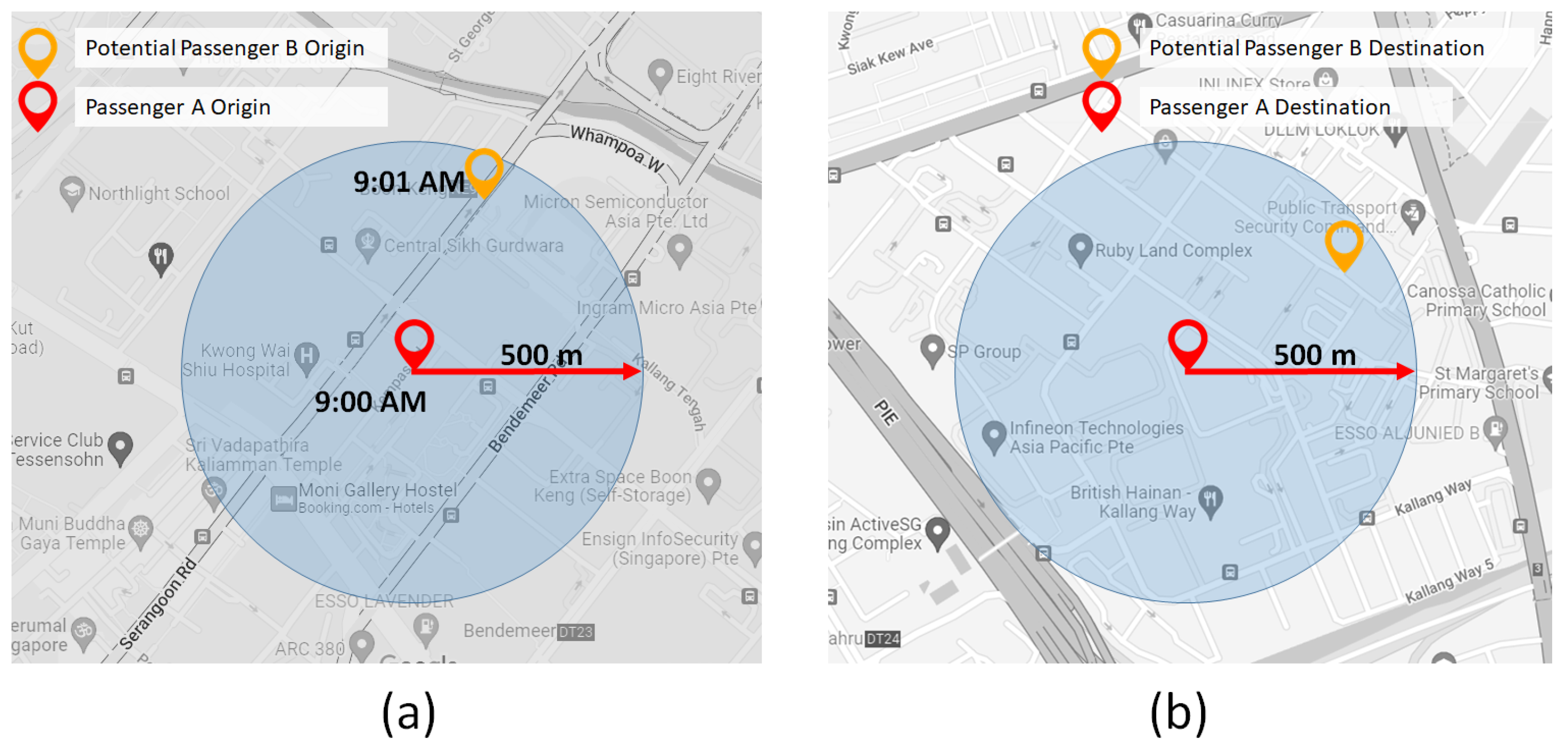
Stable matching pairs viable passengers by inspecting their trajectories and considering their spatiotemporal properties such as time frames and comparative distance separation. The following conditions, as seen in Figure 3 between Passenger A and Passenger B are set in order for them to be matched.

• Passenger B must be within 5 min of walking time of Passenger A’s time range.
• Passenger B’s origin must be within the geographic range of Passenger A set to r = 500 m.
• Passenger B’s destination must be within any point of Passenger A’s route set to r = 500 m.

Figure 3. Example Scenarios of Stable Matching (a) where a Passenger B’s origin (yellow), discovered at 9:01 a.m. and within the $r=$ 500 m of Passenger A (red) position, discovered at 9:00 a.m. and (b) Passenger B’s destination (yellow), within the $r=$ 500 m of the Passenger A (red) destination.

Figure 3. Example Scenarios of Stable Matching (a) where a Passenger B’s origin (yellow), discovered at 9:01 a.m. and within the $r=$ 500 m of Passenger A (red) position, discovered at 9:00 a.m. and (b) Passenger B’s destination (yellow), within the $r=$ 500 m of the Passenger A (red) destination.

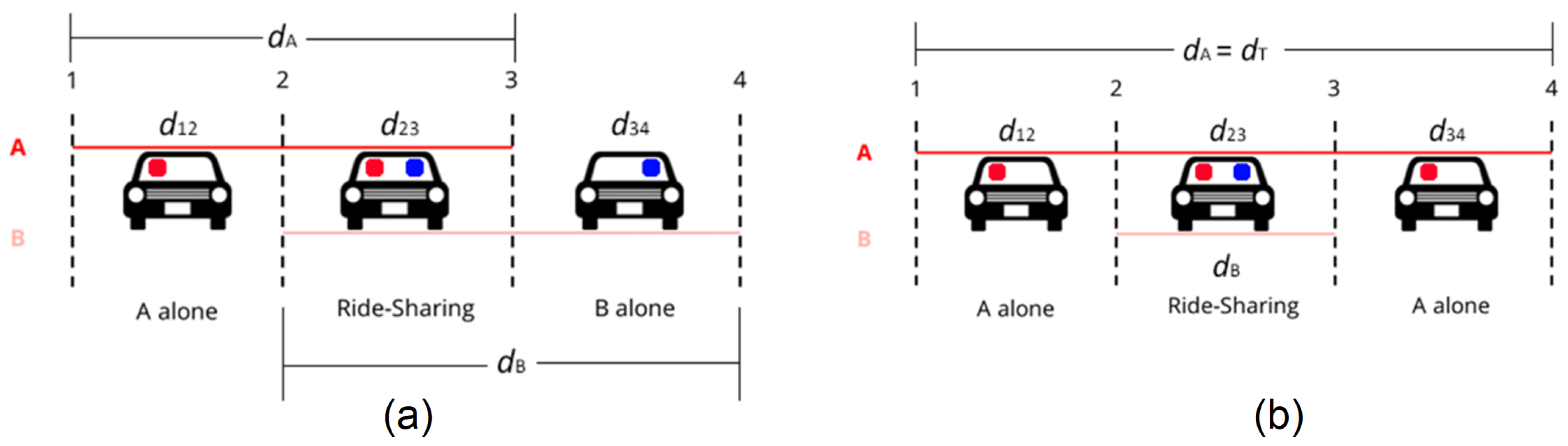
In Figure 3, we identified two possible types of stable matches, namely, Type 1 and Type 2 matches, as shown in Figure 4. In Type 1 match, Passenger B’s trip ends after Passenger A’s destination while in Type 2 Match, Passenger B’s trip will end before Passenger A arrives at its destination. The total traveled distance of the trip for either case is $d_t=d_{12}+d_{23}+d_{34}$. If the ratio of $d_{23}$ and $d_t$ approaches one, then the stable matching indicates a good pair. In Types 1 and 2, the total traveled distances of Passengers A and B are $d_A=d_{12}+d_{23}$ and $d_B=d_{23}+d_{34}$ and $d_A=d_t$ and $d_B=d_{23}$, respectively.

Given only the case where two passengers are to be paired, two methods of stable matching are proposed, namely, (1) First Come First Served (FCFS) and Best Time Sharing (BT). We will choose appropriately which Passenger B will be paired to a requesting Passenger A. Let Passenger $P_{B,n}$ be a member of the set of N possible passengers who are viable candidates to be paired with Passenger A, $P_B$ = $\left\{P_{B,1},P_{B,2},\cdots ,P_{B,n},P_{B,N}\right\}$.

In FCFS, $P_{B,n}$ has a corresponding time attribute, $T_{B,n}$, that indicates the earliest time each passenger is discovered. Among this set, the earliest passenger to request a ridesharing service after Passenger A is discovered will be chosen as its stable match. $T_{B,n}<T_{threshold}$ to provide a waiting window where Passenger A can wait for possible ridesharing. Once $T_{B,n}>T_{threshold}$, Passenger A is obliged to take a solo ride. On the other hand, in BT, Passenger B has a shared distance attribute, $D_{B,n}=\frac{d_{23,n}}{d_{t,n}}$. Among this set, the passenger with the highest shared distance is chosen as Passenger B.

We define a route, denoted by ${\theta }_A$, as a set of location points $\left\{{\eta }_o,{\eta }_1,{\eta }_i,\cdots ,{\eta }_d\right\}$ from origin (${\eta }_o$) to destination (${\eta }_d)$ points traversed by passenger A characterized by its latitude and longitude GPS coordinates. Note that given the origin and destination points of Passenger A, Dijkstra’s algorithm is used to calculate the shortest path. Each ${\eta }_i$ is also characterized by its corresponding timestamp. Stable matching in this study is defined as the pairing of routes ${\theta }_A$ and ${\theta }_B$ into a common route ${\theta }_S$ such that distance traveled by the determinant passenger A and the implicated passenger B post-match do not deviate from their unmatched distance by an acceptable margin, and whom are spatiotemporally feasible.

Each iteration of the algorithm observes a distinct ${\theta }_A$ represented as $\left\{{\theta }_{A,1},{\theta }_{A,2},\cdots ,{\theta }_{A,N}\right\}$ where N is the total number of all traces. ${\theta }_A$ is the primary route of comparison to routes ${\theta }_B=\left\{{\theta }_{B,1},{\theta }_{B,2},\cdots ,{\theta }_{B,M}\right\}$.

Passengers A and B can feasibly be stable matched if all following conditions are satisfied:

• ${\theta }_A$≠, ${\theta }_B$≠, ${\theta }_A$ ≠ ${\eta }_{A,1}$, ${\theta }_B$ ≠ ${\eta }_{B,1}$
• Passenger B is a member of set $\left\{B_{wt}=B_{wt,1},B_{wt,2},\cdots ,B_{wt,M}\right\}$, where $B_{wt}$ is the set of all passenger B whose origin time is greater than or equal to origin time of passenger A but less than destination time of passenger A.
• Passenger B has origin within set haversine distance r [40] from any point within ${\theta }_A$. This nearest point of pickup is then denoted as ${\eta }_B$. The haversine distance r is obtained by:

  $$\begin{array}{cc}\hfill r& =6371c\hfill \\ \hfill c& =arctan2\left(\sqrt{a},\sqrt{1-a}\right)\hfill \\ \hfill a& =si{n}^2\left(\frac{{\varphi }_2-{\varphi }_1}{2}\right)+cos{\varphi }_{1}cos{\varphi }_{2}si{n}^2\left(\frac{{\lambda }_2-{\lambda }_1}{2}\right)\hfill \end{array}$$

  where ${\varphi }_x$ and ${\lambda }_x$ are the latitudes and longitudes of the point x, respectively.
• Passenger B has destination within set haversine distance r from any point within ${\theta }_A$, but whose index within ${\theta }_A$ must be greater than the index of ${\eta }_B$ within ${\theta }_A$.

The discussion of the stable matching procedures is shown in Algorithm 1.

Once all possible pairings have been obtained, Algorithms 2 and 3 then determine which pairings will be accepted such that no trip is duplicated between matches. The outputs are ${\mu }_{FCFS}$ and ${\mu }_{BT}$ which contain the set of all rideshare pairings based on discovery time and shared passenger distance relative to overall distance while accounting for unique taxi IDs.

Algorithm 1: Stable Matching All Possible Pairs.

INPUT: OD pairs—List of all trajectories to be stable-matched for each trace do     $traceID1$ = current index’s traceID     $startLoc1$ = current index’s starting location     $stopLoc1$ = current index’s stop location     Get shortest path from startLoc1 to stopLoc1     path1 = convert nodes to equivalent coordinate     if route is not null and not singular then         Find all traces within acceptable time         for each trace within acceptable time do            $traceID2$ = current index’s traceID            $startLoc2$ = current index’s starting location            $stopLoc2$ = current index’s stop location            if $traceID1$≠$traceID2$ then                if $startLoc2$ lies within 500 m of any node of path1 then                    if $stopLoc2$ is within range of any node of path1 then                        $matchPath$ = create dijkstra path from $startLoc1$ to $startLoc2$                        if $stopLoc2$ is within 500 m of $stopLoc1$ then                           $d_{12}$ = Dijkstra path length from $startLoc1$ to $startLoc2$                           $d_{23}$ = Dijkstra path length from $startLoc2$ to $stopLoc1$                           $d_{34}$ = Dijkstra path length from $stopLoc1$ to $stopLoc1$                           Compute overall ride-share distance                           Create dijkstra path length for $traceID1$ and $traceID2$                           Save IDs, start time, pertinent points, distance, type 1 info                        else if $stopLoc2$ is within 500 m of path1 then                           $d_{12}$ = Dijkstra path length from $startLoc1$ to $startLoc2$                           $d_{23}$ = Dijkstra path length from $startLoc2$ to $stopLoc2$                           $d_{34}$ = Dijkstra path length from $stopLoc2$ to $stopLoc1$                           Compute overall ride-share distance                           Create Dijkstra path length for $traceID1$ and $traceID2$                           Save IDs, start time, pertinent points, distance, type 2 info                        end if                    end if                end if            end if         end for     end if end for OUTPUT: $\mu =d_{12}\cup d_{23}\cup d_{34}$

Algorithm 2: First Come First ServeD (FCFS) Matching Algorithm.

INPUT: MainTable1— list of $\mu$ derived from Algorithm 1 Sort MainTable1 by start time for each trace in MainTable1 do     if $traceID1$ and $traceID2$ are not recorded in table MainTable2 then         Record pair to MainTable2     else         Discard pair     end if end for OUTPUT: ${\mu }_{FCFS}$ = MainTable2

Algorithm 3: Best Time Sharing (BT) Matching Algorithm.

INPUT: MainTable1—list of $\mu$ derived from Algorithm 1 for each trace in MainTable1 do     shareWeight = $\frac{d_{23}}{d_t}$ end for Sort MainTable1 by shareWeight for each trace in MainTable1 do     if $traceID1$ and $traceID2$ are not recorded in table MainTable2 then         Record pair to MainTable2     else         Discard pair     end if end for OUTPUT: ${\mu }_{BT}$ = MainTable2

3.2. Solo Ride Pricing Structure

The basic pricing method for a solo-riding passenger used in this work is given by (1). The cost function of a ride, $\sigma$, is only dependent on the total distance, $d_t$, traveled. The total distance is multiplied by the running rate ($\delta$), then, added to the base fare ($ϵ$) to constitute the ride’s total cost. These two variables vary depending on the city under study.

$$\sigma =ϵ+\delta d_t$$

(1)

Table 2. Fare Table Matrix.

Location	Base Fare ($\mathit{ϵ}$)	Running Cost ($\mathit{\delta }$)
Jakarta (Sep 2018)	22.10 PHP	10.20 PHP/km
Singapore (Dec 2018)	88.67 PHP	7.73 PHP/km
New York (Dec 2013)	97.37 PHP	44.01 PHP/km

illustrates the rates of each city converted to Philippine Pesos (PHP) as a common currency. Tips and time-based fares are not included for simplicity and uniformity across all three cities. Time-based fares are those fare adjustments when the taxi is stuck in traffic jams and changes after a predefined time with no mobility.

3.3. Ridesharing Pricing Techniques and Overall Benefit

We discuss in this section various ridesharing pricing techniques that will all be compared to the solo ride pricing structure.

3.3.1. Equal-Split (ES) Pricing

Equal-split (ES) pricing involves charging both Passengers A and B an amount equivalent to half of the cost function regardless of the distance each passenger has traveled while completing the route. This is regardless of the ridesharing type. The fare cost per passenger, denoted by $P_{A,ES}$ and $P_{B,ES}$, respectively, is shown in (2).

$$P_{A,ES}=P_{B,ES}=\frac{\sigma }{2}$$

(2)

Evidently, the passenger who travels longer receives a higher benefit because the passenger has utilized the ride longer yet still pays the same amount as the other passenger. On the other hand, it is still guaranteed that both passengers will be paying an amount smaller than when they did solo-ride.

The driver’s revenue remains unchanged since he still receives the same had he/she served just one passenger with the same route. In this method, the driver neither benefits nor is at a disadvantage.

3.3.2. Proportional-Split (PS) Pricing

In Proportional-split (PS) pricing, a Passenger A pays a fare that is proportional to the distance traveled. Under a Type 1 match, Passenger A only pays the cost from point 1 to point 3, while passenger B pays only the proportional distance covered by point 2 to point 4. (See Figure 4).

The total cost of the ride, $\sigma$, given in (3), is broken into three segments representing the three sections of the complete route. $\alpha ,\beta ,$ and $\gamma$ are the costs of the first, second, and third sub-routes comprising the total route with distance $d_t$.

$$\begin{array}{cc}\hfill \alpha & =\sigma \ast \frac{d_{12}}{d_t}\hfill \\ \hfill \beta & =\sigma \ast \frac{d_{23}}{d_t}\hfill \\ \hfill \gamma & =\sigma \ast \frac{d_{34}}{d_t}\hfill \\ \hfill \sigma & =\alpha +\beta +\gamma \hfill \end{array}$$

(3)

For Types 1 and 2 matches, the fares paid by Passengers A and B, $P_{A,PS}$ and $P_{B,PS}$ are given in (4) and (5), respectively.

$$P_{A,PS}=\alpha +\beta P_{B,PS}=\beta +\gamma ,d_B\ne d_{23}$$

(4)

$$P_{A,PS}=\alpha +\beta +\gamma P_{B,PS}=\beta ,d_B=d_{23}$$

(5)

The driver revenue, for either Type match, is simply given by $P_{D,PS}=P_{A,PS}+P_{B,PS}=\alpha +2\beta +\gamma$. Given the PS pricing scheme, the driver gains an additional profit because there is a double payment made by the passengers due to distance $d_{23}$.

3.3.3. Game Theory (GT) and Nash Equilibrium

We propose a GT-based pricing method that takes both properties of equal-split and proportional split pricing techniques. When a passenger is alone during the ridesharing, he/she will only have to pay the corresponding fare for those sections of the ride, but when both passengers are now simultaneously riding the vehicle, fares during that portion will be evenly split among them. The cost functions for both Passengers A and B for Type 1 and Type 2 stable matching are given in (6) and (7), respectively. The driver profit is $P_{D,PS}=P_{A,PS}+P_{B,PS}=\alpha +\beta +\gamma$, which is the same as Equal-Split ridesharing.

$$P_{A,GT}=\alpha +\frac{\beta }{2}{P}_{B,GT}=\frac{\beta }{2}+\gamma ,d_B\ne d_{23}$$

(6)

$$P_{A,GT}=\alpha +\frac{\beta }{2}+\gamma P_{B,PS}=\frac{\beta }{2},d_B=d_{23}$$

(7)

We utilize the price per kilometer as the main metric for measuring Nash Equilibrium. For drivers, the optimal situation is to have an average increase in PHP/km of revenue. Moreover, drivers are getting more rewards for the same level of service. On the other hand, passenger benefit is measured by the degree of reduction in PHP/km paid for rides, as this signifies an overall cost efficiency in terms of the cost of service. Generating a strategy which addresses these conflicting interests is the main target of the study. To achieve a state of Nash Equilibrium, each individual (e.g., Driver, passengers) forming the group must believe that it is each in their best interest to conform with the common strategy (i.e., sharing a ride instead of riding alone). From all possible strategies a player i can employ ($S_i$), it can be said that a chosen strategy is the best if the utility ${\mu }_i\left(s_i\right)$ of that selected strategy $s_i$ outweighs the utility obtained by all other possible strategies ${\mu }_i\left(s_i^{*}\right)$, considering all the other players’ best possible strategies $s_i^{*}$. When the best strategy of one individual is aligned with the best strategies of his peers in a group, then Nash Equilibrium is achieved. Mathematically, this is represented by ${\mu }_i\left(s_i\right)\ge {\mu }_i\left(s_i^{*}\right),\forall s_i\in S_i$.

3.3.4. Nash Score

We compare the overall benefit by computing for the Nash Score of all pricing models. This is obtained by taking the arithmetic mean of all three Aggregate Benefit values. In other words, this is the average benefit of all three pricing models under a given stable matching method under a specified city. Comparing Nash Scores across cities and stable matching methods of the same city is a satisfactory indicator as to which stable matching method is best, and which city is most conducive to ridesharing. Equation (8) gives the Nash score for a pricing model.

$$\omega =\frac{{\phi }_{ES}+{\phi }_{PS}+{\phi }_{GT}}{3}$$

(8)

where $\omega$ is the Nash Score of a specific stable matching algorithm and ${\phi }_{xx}$ is the aggregate benefit (sum of the benefits of the Driver, Passenger A, and Passenger B) obtained under a specific pricing model.

4. Results

In this section, we present the results of our extensive simulations and further evaluation of our proposed system using the empirical mobility dataset traces from the three cities. We analyzed the efficiency of our stable matching algorithm and pricing models compared to a no ridesharing benchmark.

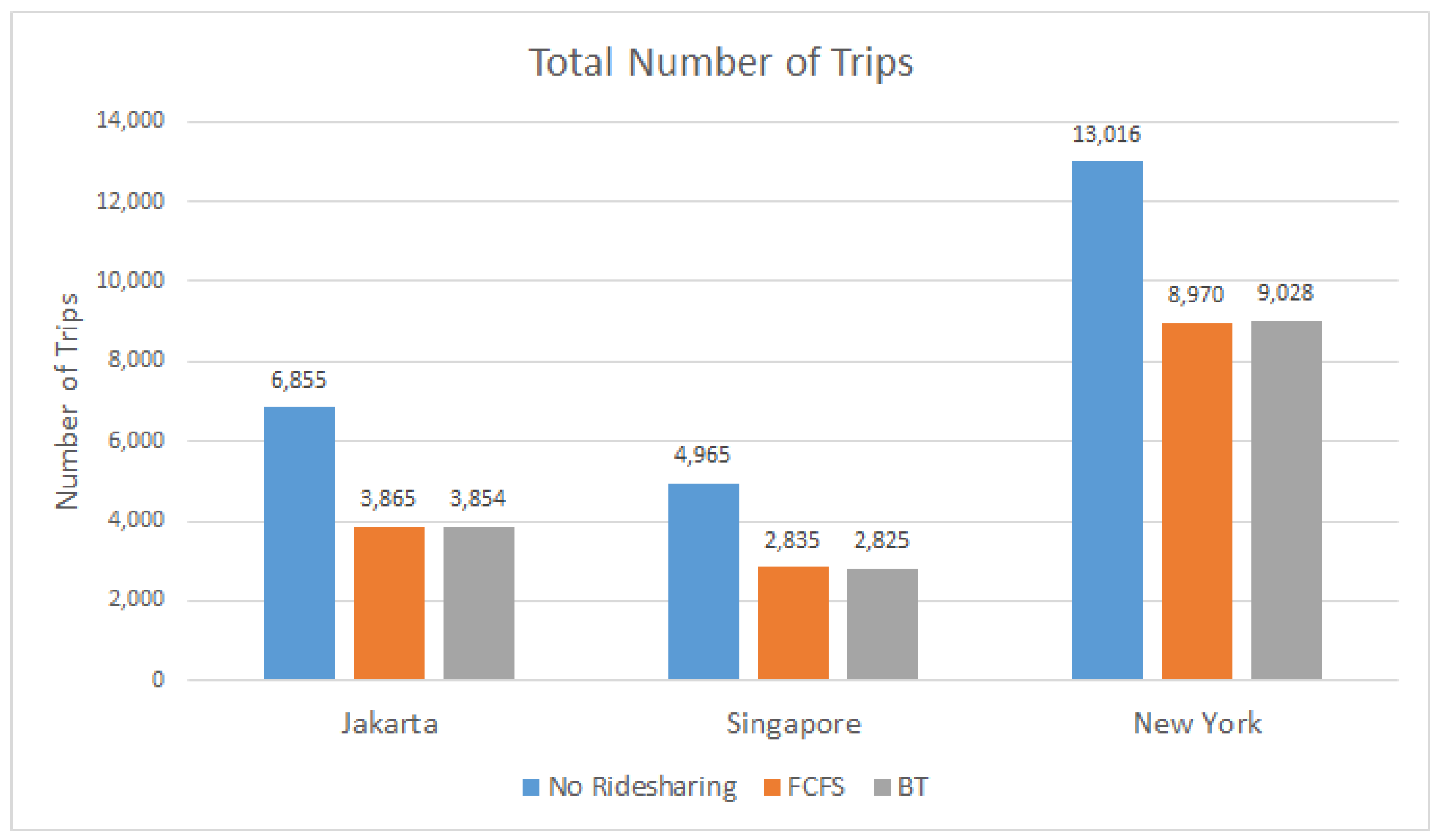
4.1. Number of Feasible Ridesharing Passengers Matched

Figure 5 presents the total number of trips for all the possible passengers under no ridesharing, FCFS, and BT matching. There is at least a 30% reduction in the number of trips when commuters come together in the three observed cities. Aside from the advantages discussed in this work, this ridesharing method is also beneficial to the environment. Even though we have a reduction in the number of trips, one must think that other taxis can be optimally assigned to other ridesharing commuters. Figure 5 also provides an overview of the effectiveness the proposed stable matching algorithms in further reducing the number of trips by a significant amount which effectively ease the vehicle congestion in these three key cities.

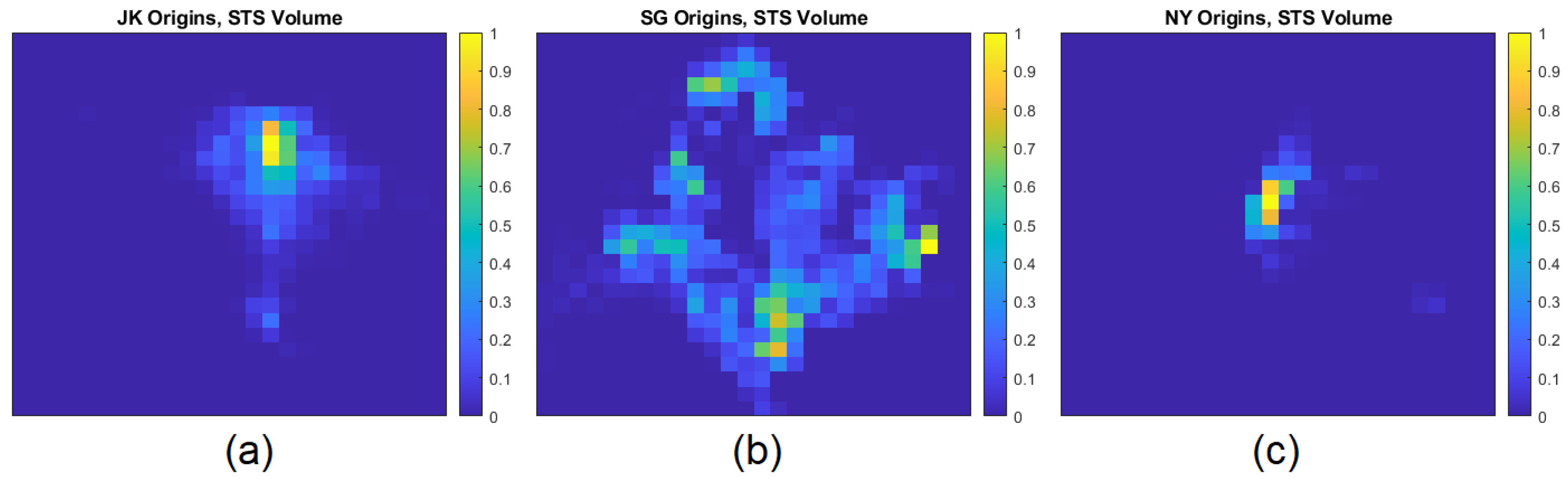
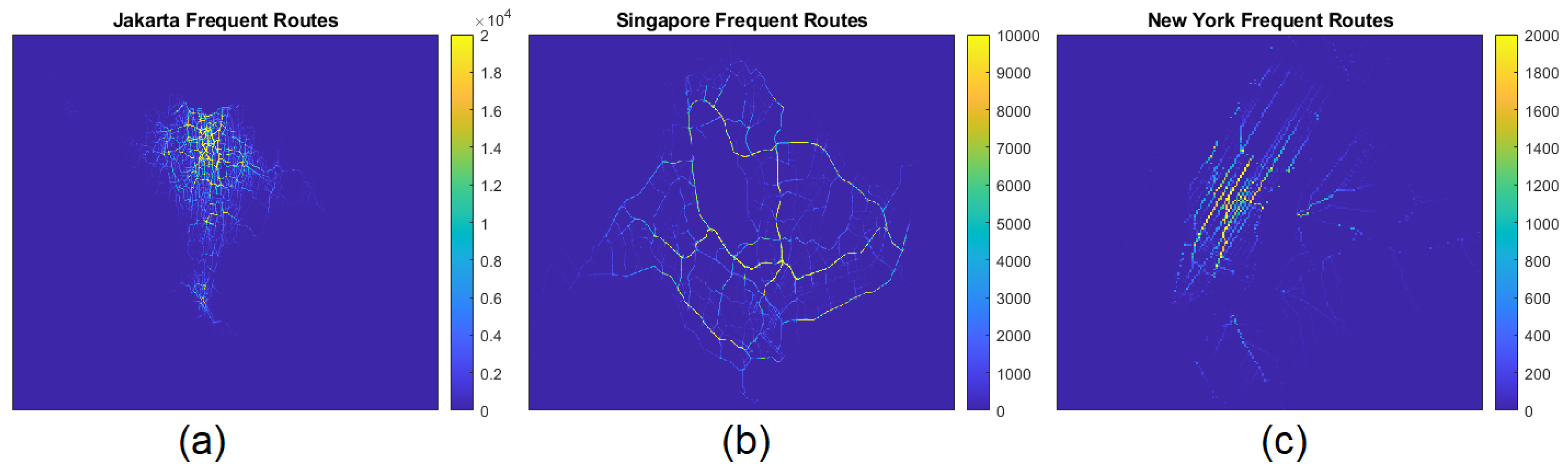
From these no ridesharing number (blue bar of Figure 5), FCFS and BT stable matching methods have paired nearly 90%, 86%, and 60% of all possible passengers, in Jakarta, Singapore, and New York, respectively. We also observed that the ridesharing requests are scattered more in Jakarta and Singapore as compared to New York which can be found denser in almost the central Manhattan borough.

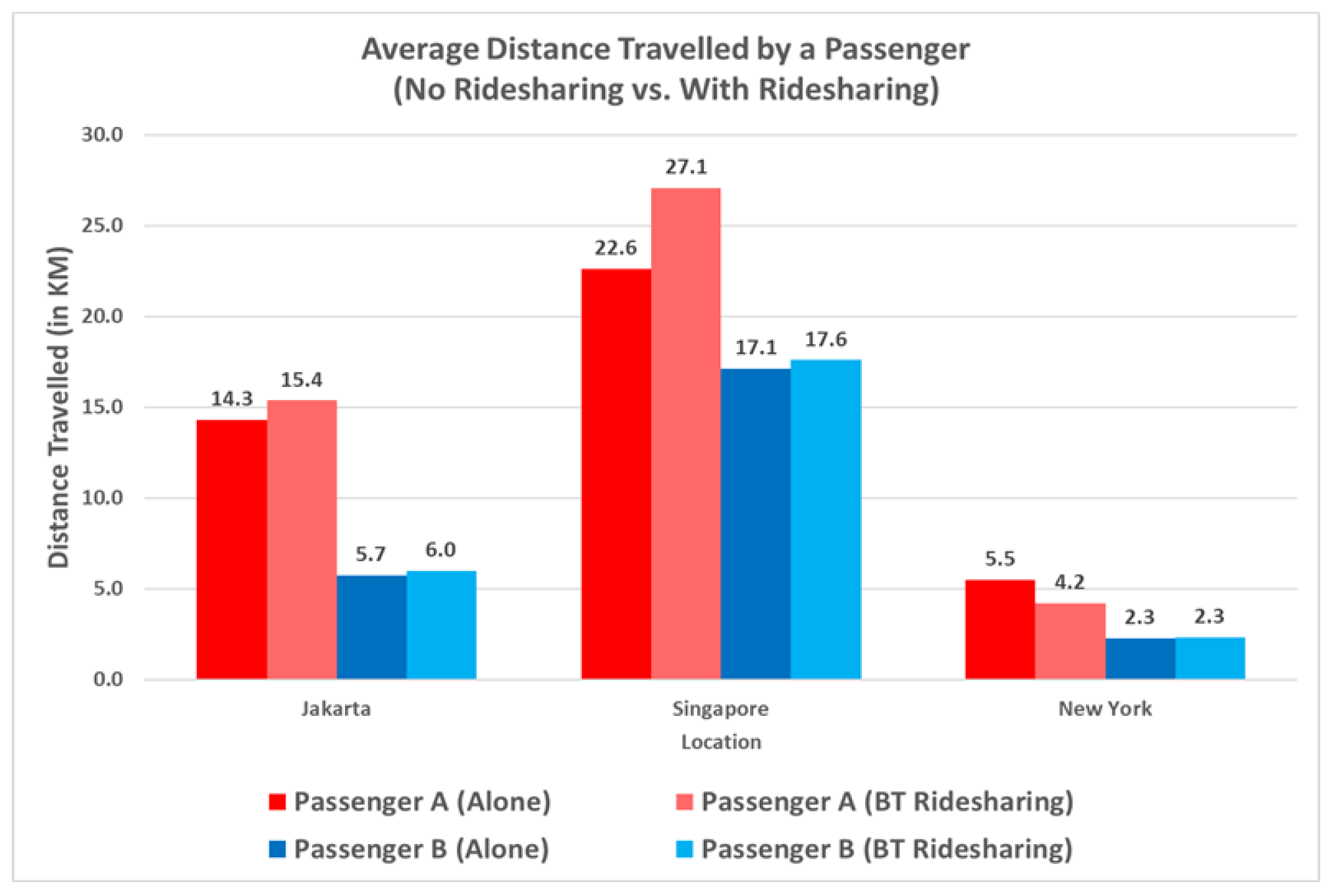
4.2. Average Travel Distance

An inherent drawback of ridesharing is an increase in riding distance because of the generation of a new route that accommodates both passengers involved. Taking this fact into consideration, riding alone is more straightforward in terms of distance. This is shown in Figure 6. However, Best Time Stable Matching has made it such that this increase in distance is minimized such that riders still feel highly encouraged to carpool with another passenger. The highest increase in distance observed was Passenger A in Singapore (20%). Other than this, distance increases have only been confined to 2–7%. In New York, a 24% decrease in distance was observed. It can be suggested that Best Time Matching was able to generate better routes for both passengers, such that it was even an improvement to riding alone.

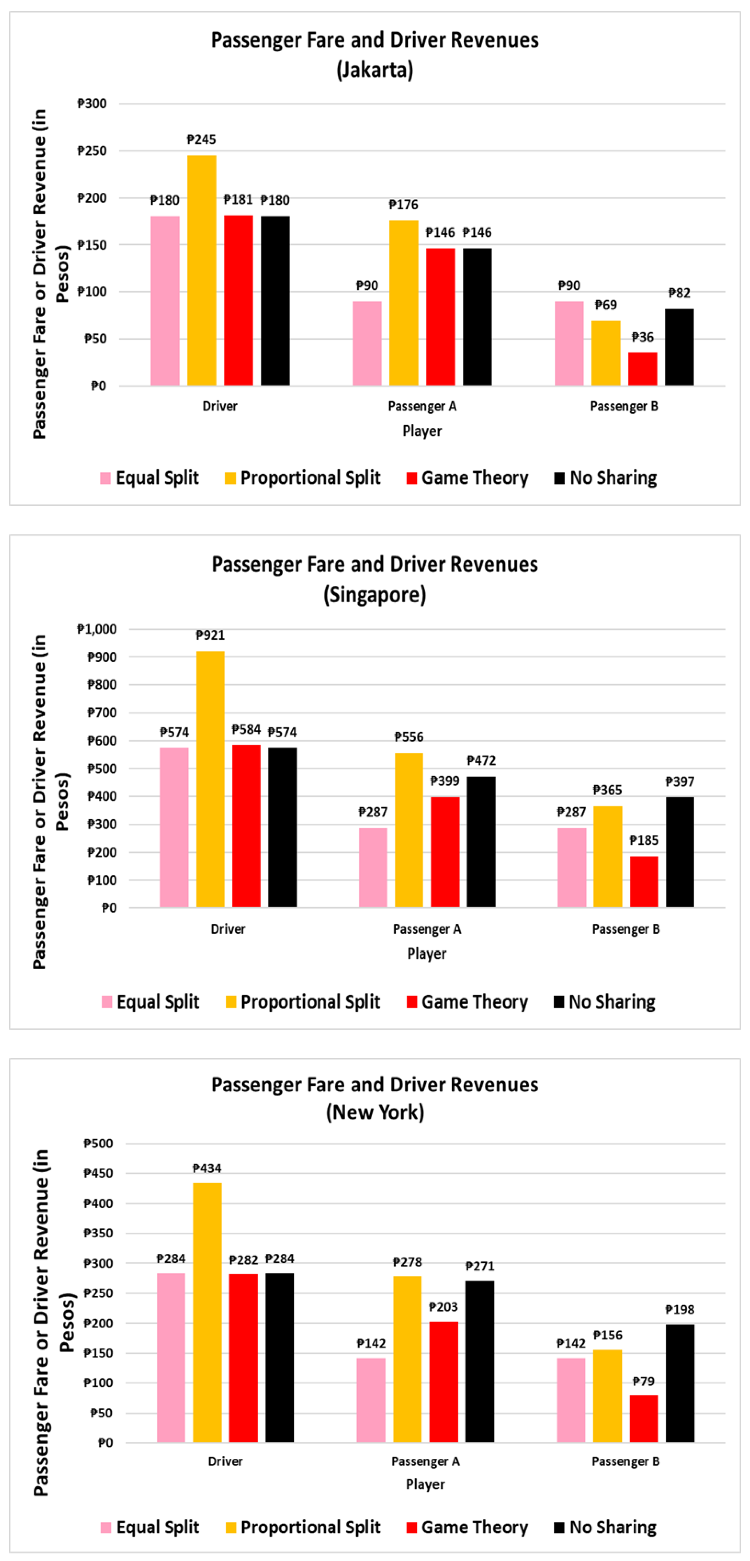
4.3. Average Passenger Fare and Driver Revenues

Figure 7 shows the passenger fare and driver revenue under various ridesharing and no ridesharing schemes.

In Jakarta, drivers benefited the most in the PS pricing, having obtained an additional PHP65 of revenue from the benchmark of P180 under no ridesharing. However, under ES and GT pricing, the driver yielded almost little to no additional revenue. Passenger A was the losing party under PS pricing, having to pay an additional PHP30 in fare. This was a result of the addition in distance due to ridesharing being experienced by both passengers. Whereas under ES, Passenger A is greatly favored, needing only an average of PHP56 in fare as compared to paying an average of PHP146 when riding alone. Meanwhile, GT pricing provided no net discount for Passenger A. As for Passenger B, this entity greatly benefited, as shown by the biggest cost reduction in terms of proportion. ES pricing served the least favorable, with Passenger B having to pay an additional PHP8 from the average solo riding fare. This is due to both Passenger A and B equally dividing the fare despite the latter riding shorter trips on average. Under PS, the fare was reduced from PHP82 to PHP69, and a more significant decrease was seen under GT pricing, only having to pay PHP36 on average. GT pricing served as a gain for Passenger B because it only paid the proportion of the total ride it was inside the vehicle. Moreover, when both passengers were in the ride, Passenger B only paid half of that proportion with assisted in the reduction of costs.

In Singapore, PS pricing heavily favored the driver and is detrimental to Passenger A. This benefit on the driver’s side is caused by the shared distance of both passengers. Meanwhile, Passenger B’s fare slightly decreased under PS pricing due to the ride distance not being adversely affected, just as in Jakarta. ES Pricing yielded no benefit to the driver and Passenger A still received the biggest benefit. Unlike in Jakarta, however, Passenger B’s fare did not see an increase. The benefits it obtained by ridesharing were enough to offset the negative effects it incurred from ES Pricing. Much like Jakarta, GT Pricing served as the most beneficial as it gave a slight additional revenue to the driver (PHP10), Passenger A having a PHP73 fare reduction, and Passenger B had its fare cut by more than half of the original fare (PHP212).

New York’s statistics had the most favorable results as each pricing method was able to deliver benefits to at least two Players without undermining the other remaining Player. Under ES Pricing, Passenger A and B’s fare we reduced by nearly 50% and 40%, respectively. Meanwhile, in PS Pricing, only Passenger A experienced an increase in fare, but only on a minimal scale. This is because some rides still posted longer trip distances for Passenger A when ridesharing than when alone.

5. Discussion

Given the fare and revenue distributions in the previous section, we now analyze and discuss the benefits brought about by the proposed ridesharing methods.

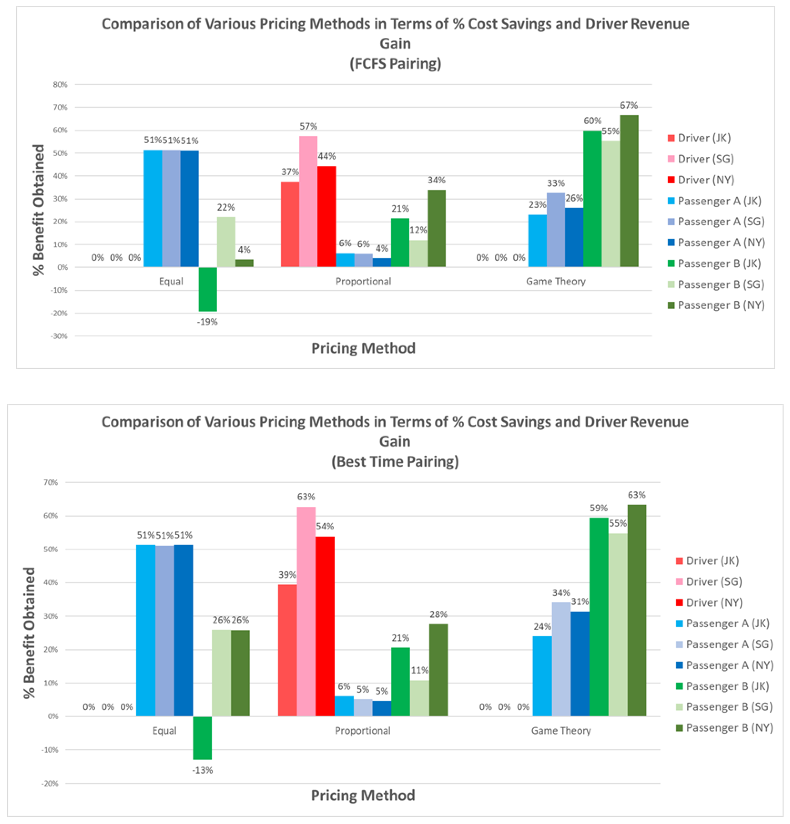
5.1. Distribution and Cost Equitability of Benefits among Players

In terms of cost equitability and distribution of benefits, the three pricing techniques yielded varying results, as shown in Figure 8. ES Pricing is shown to benefit Passenger A the most; however, this is done at the expense of Passenger B having negative benefit. This creates a Zero-Sum Game wherein one player’s benefit comes at the expense of another. Furthermore, it only lowered Passenger A’s cost in relative terms due to it paying the same amount despite having a longer travel distance than Passenger B.

On the other hand, PS Pricing can be considered as more cost equitable due to all three players receiving at least some amount of additional revenue. The driver received the most benefit in this technique, primarily driven by the double revenue it collected during the portion of the ride where both Passengers A and B are simultaneously in the vehicle. As for both passengers, a modest amount of benefit is seen for the total ride cost only involving one base charge. Passenger B’s benefit is greater than Passenger A due to the former’s shorter travel distance. The derivation of passenger cost savings indicate that base fares have a greater impact on rides having shorter distances.

However, in terms of overall and general benefit, GT Pricing exhibited this most among the three pricing techniques. Passenger B experienced a reduction in fare by at least 50% and Passenger A had a significant decrease as well ranging from 24–34%. It is possible because under GT, the sharing cost Passengers A and B is halved, and resulted in obtaining greater discounts compared with PS Pricing. This also resulted in the driver receiving minimal to no additional revenue. Despite this, the magnitude of discounts both Passengers A and B received considerably outweighed the absence of driver revenue.

5.2. Nash Scores

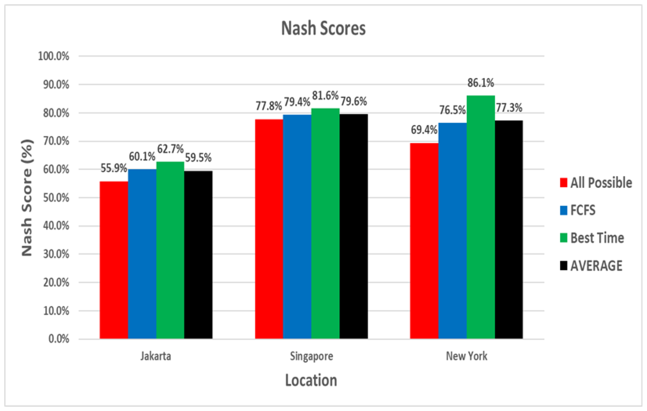
The Nash Score, shown in Figure 9, compares the average benefits obtained by different Stable Matching methods presented in (8). For instance, a Nash Score of 81.6% obtained in the Singapore dataset using Best Time Pairing is derived from the total benefits obtained under ES, PS, and GT Pricing which are 77.04%, 78.87%, and 88.87%, respectively. The average of these three is 81.6%.

Across all three cities, BT Stable Matching produced the highest Nash Scores because BT allows paired passengers to maximize their time together inside the vehicle, effectively, maximizing the shared distance leading to the most cost savings.

Singapore has the highest average Nash Score (79.6%) and suggests that it has the most conducive location for ridesharing. However, when a one uses the BT Stable Matching method only in any of these three cities, New York is the most conducive, posting a Nash Score of 86.1%. Using Best Time Pairing in New York succeeded mainly because of its grid-type roads and straightforward paths. Another key factor is also the ease of pairing passengers due to the fact that the pool of possible pairs is mostly confined in just the Manhattan area (which has a land area of only 59.1 km${}^2$). This is unlike Jakarta and Singapore with 661.5 and 728.6 km${}^2$ of land area, respectively.

5.3. Extending Ridesharing Schemes to More Than Two Passengers

Our evaluation of various pricing schemes can be modified to accommodate 3–4 passengers. Given the First Come First Served (FCFS) stable matching method, we select the first three earliest passengers, instead of only one passenger. On the other hand, for Best Time Sharing (BT) stable matching method, we get the three highest shared distance among the set of all possible passenger choices.

For the ridesharing pricing techniques, the following evaluation will change accordingly. For the equal split sharing, we have:

$$P_{1,ES}=P_{2,ES}=\cdots =P_{x,ES}=\frac{\sigma }{x}$$

(9)

where $x=3,4$ depending on the number of passengers sharing the ride.

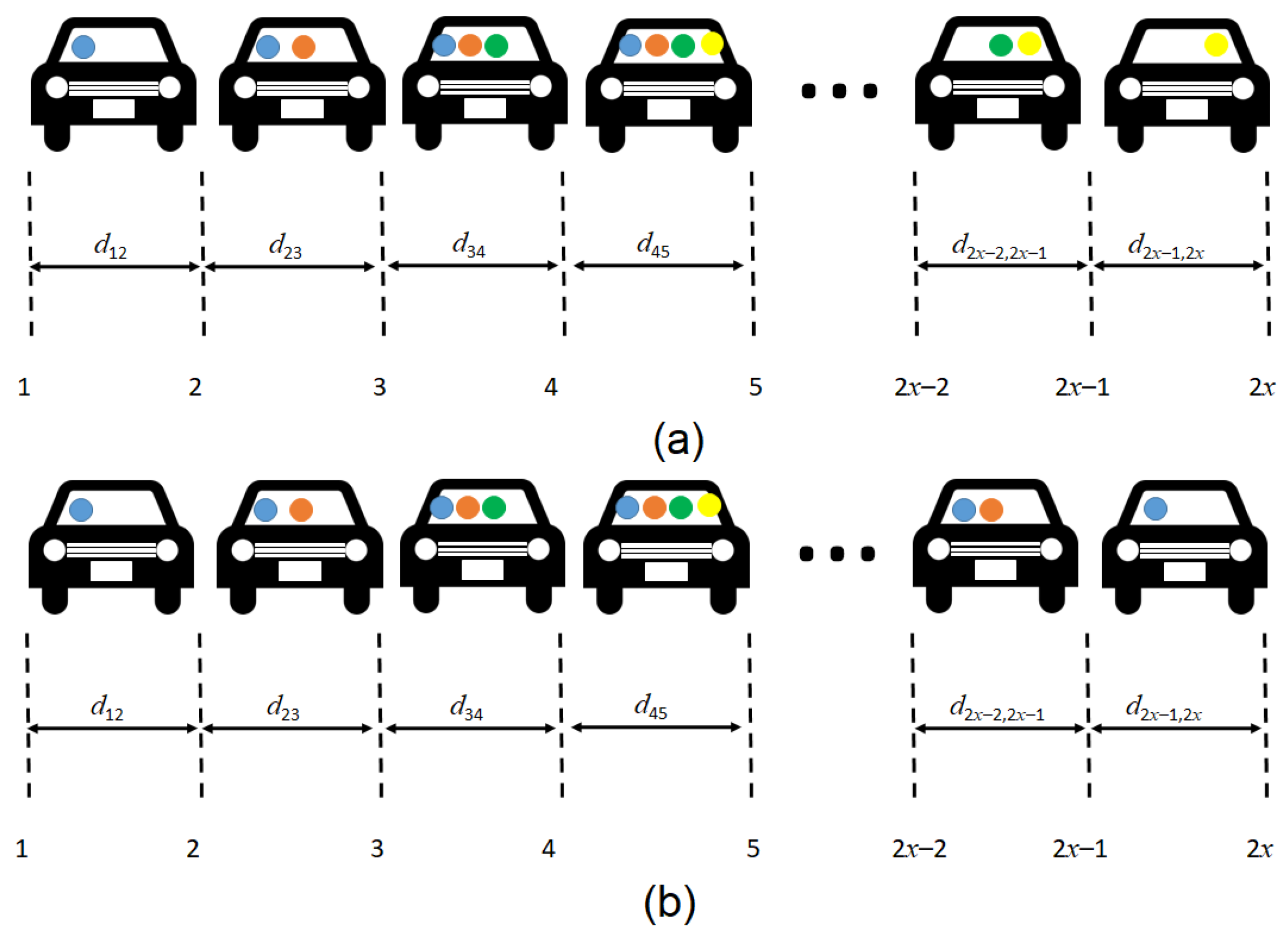
Figure 10 shows the extended illustration to accommodate x ridesharing passengers. There are exactly $2x$ unique points to consider during the ridesharing process.

For proportional split pricing, we have:

$$\begin{array}{cc}\hfill {\alpha }_{12}& =\sigma \ast \frac{d_{12}}{d_t}\hfill \\ \hfill {\alpha }_{23}& =\sigma \ast \frac{d_{23}}{d_t}\hfill \\ \hfill ⋮\\ \hfill {\alpha }_{2x-2,2x-1}& =\sigma \ast \frac{d_{2x-2,2x-1}}{d_t}\hfill \\ \hfill {\alpha }_{2x-1,2x}& =\sigma \ast \frac{d_{2x-1,2x}}{d_t}\hfill \\ \hfill \sigma & ={\alpha }_{12}+{\alpha }_{23}+\cdots +{\alpha }_{2x-1,2x}\hfill \end{array}$$

(10)

For Types 1 and 2 matches, the fares paid by the passengers involved in each of the stable matching are given in (11) and (12), respectively.

$$P_{i,PS}={\alpha }_{i,i+1}+\cdots +{\alpha }_{i+x-1,i+x}$$

(11)

$$\begin{array}{cc}\hfill P_{x,PS}& ={\alpha }_{x,x+1}\hfill \\ \hfill P_{x-1,PS}& ={\alpha }_{x-1,x}+P_{x,PS}+{\alpha }_{x+1,x+2}\hfill \\ \hfill ⋮\\ \hfill P_{1,PS}& ={\alpha }_{12}+P_{2,PS}+{\alpha }_{2x-1,2x}\hfill \end{array}$$

(12)

For the proposed Game Theory-based pricing, the cost functions for the passengers involved in Type 1 and Type 2 stable matching are given in (13) and (14), respectively.

$$P_{i,GT}=\frac{{\alpha }_{i,i+1}}{x}+\cdots +\frac{{\alpha }_{i+x-1,i+x}}{x}$$

(13)

$$\begin{array}{cc}\hfill P_{x,GT}& =\frac{{\alpha }_{x,x+1}}{x}\hfill \\ \hfill P_{x-1,GT}& =\frac{{\alpha }_{x-1,x}}{x-1}+P_{x,PS}+\frac{{\alpha }_{x+1,x+2}}{x-1}\hfill \\ \hfill ⋮\\ \hfill P_{1,GT}& ={\alpha }_{12}+P_{2,PS}+{\alpha }_{2x-1,2x}\hfill \end{array}$$

(14)

where $x=$ 1, 2, 3, or 4.

We note that in general, as the number of ridesharing passengers increases, the fares of each passenger is reduced. However, aside from the financial effect of such many ridesharing passengers, we could also analyze the situation in terms of passenger convenience, waiting time, comfort, and other important travel parameters. These can be studied through empirical surveys to determine the passenger preference and travel rating.

5.4. Limitations of the Study

Our work has successfully implemented stable matching between riding passengers and executed a GT-based pricing scheme to reduce the travel cost of the passengers involved. We enumerate below some of the study’s limitations and future research directives.

• The results of our study have been highly dependent on the available GPS mobility traces of each urban city. As such, to prevent biases, our evaluation window has been limited to only 30 min a day and does not even cover peak travel/commute hours.
• Our ridesharing simulations only considered a pair of passengers and have not investigated when three to four passengers are able to rideshare. We have then enumerated the financial evaluations in Section 5.3 for future reference. Given our 30-min evaluation window too, our computation complexity is still polynomial time.
• Our study focused only on the passenger fare reduction and lacked on the analysis and evaluation of the passengers’ comfort, on-time departure and arrival at the rendezvous and drop-off points, travel comfort and convenience. Therefore, our work did not include the fare reduction-comfort relationship study to gauge the worthiness of ridesharing.

6. Conclusions

In this work, we have proposed two stable matching techniques that account for the temporal separation (i.e., First Come First Served (FCFS) method) and shared distance (i.e., Best Time Sharing (BT) scheme) between possible ridesharing passengers. Effectively, the stable matching techniques have significantly reduced running trips at a given time, especially during peak hours. BT has generated shorter average trips than FCFS because it has prioritized more overlaps among passengers, therefore, not much additional distance is necessary.

From all these stable matches, we evaluate the cost benefit achieved by each rider and driver given the solo-ride, equal (ES), and proportional (PS) splitting fare computation. ES became most beneficial to Passenger A, but at the expense of Passenger B. On the other hand, PS strongly favored drivers due to a large increase in revenue because of over payment caused by overlapping traveled distance. In these two methods, the no-ridesharing fare has still been reduced. We, then, formulated a Game Theory-based (GT) pricing technique that focuses on adjusting the passenger fares based on common distances covered during the travel. In terms of post stable matching, cost-savings, successful matches, and total number of trips, BT-GT tandem achieved the highest Nash scores, therefore, the most benefits to passengers, while introducing tolerable gains to the driver. Under our GT pricing technique, the sharing cost is halved and resulted to passengers obtaining greater costs discounts than PS. Even though drivers obtained minimal additions in revenue under GT, this was greatly outweighed by the magnitude of fare discounts acquired by both passengers.