
An Adaptive Route Planning Method of Connected Vehicles for Improving the Transport Efficiency


Abstract
:1. Introduction
- (1)
- To the best of our knowledge, we innovatively introduce for the first time a bidding mechanism to dynamically coordinate plan routing schemes for vehicles affected by congestion based on the road intersection planning center model. In this mechanism, the independent route-planning schemes of control centers in a centralized framework are transformed into a route-negotiation process of multiple CVs and road segment agents, resulting in a traffic efficiency improvement in the road network.
- (2)
- Individual and global vehicle travel times are considered simultaneously when determining bidding prices in the model, which balances the benefits of individual vehicles and global efficiency in route-planning processes. Thus, the proposed method can improve the overall traffic efficiency while avoiding congestion for individual vehicles.
- (3)
- A novel priority-set-based local search algorithm is proposed to address the combination assignment problem between large-scale traffic flow and road segments in the bidding-based route-replanning process. This algorithm improved the efficiency of route replanning by selecting a combination of winning schemes rather than a single one.
- (4)
- The remainder of this paper is organized as follows. Section 2 outlines the dynamic route-planning process. The proposed method for dynamic route planning according to the bidding mechanism is described in Section 3. Section 4 reports the methods and results of the simulation case experiments conducted to analyze the routing schemes and computational efficiency of the proposed method. Finally, Section 5 presents the discussion and conclusions of this study.
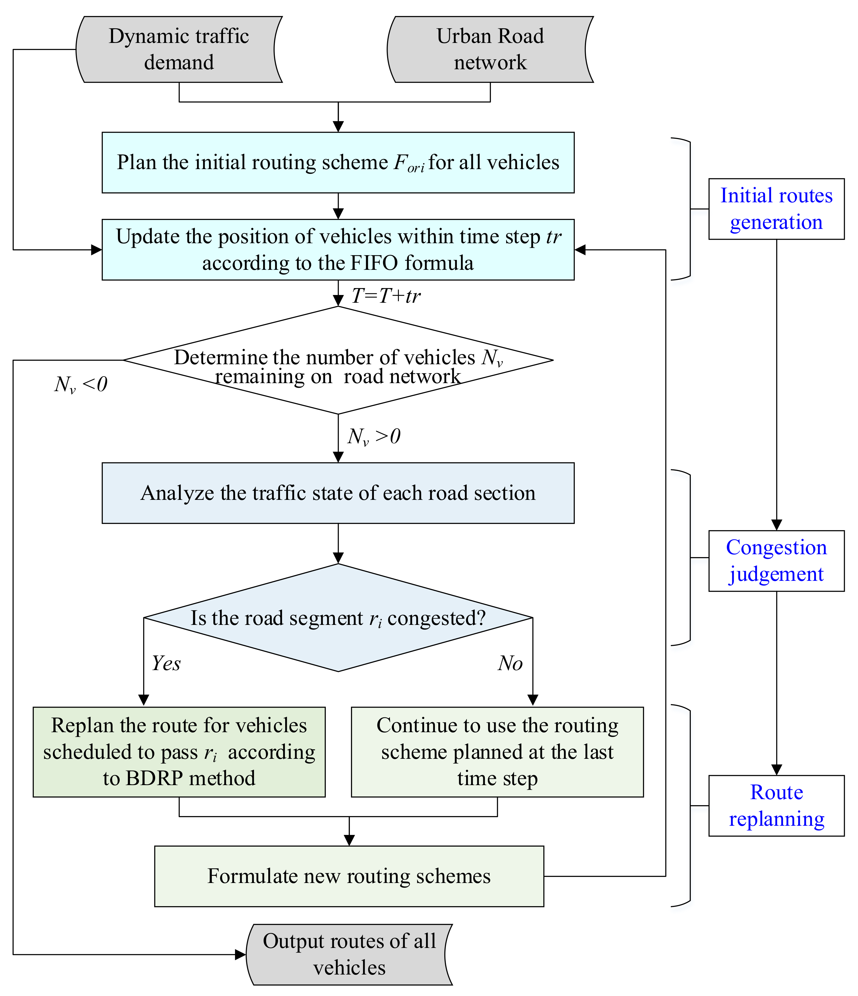
2. Dynamic Route-Planning Method Overview
3. Bidding-Based Dynamic Route-Planning (BDRP) Method
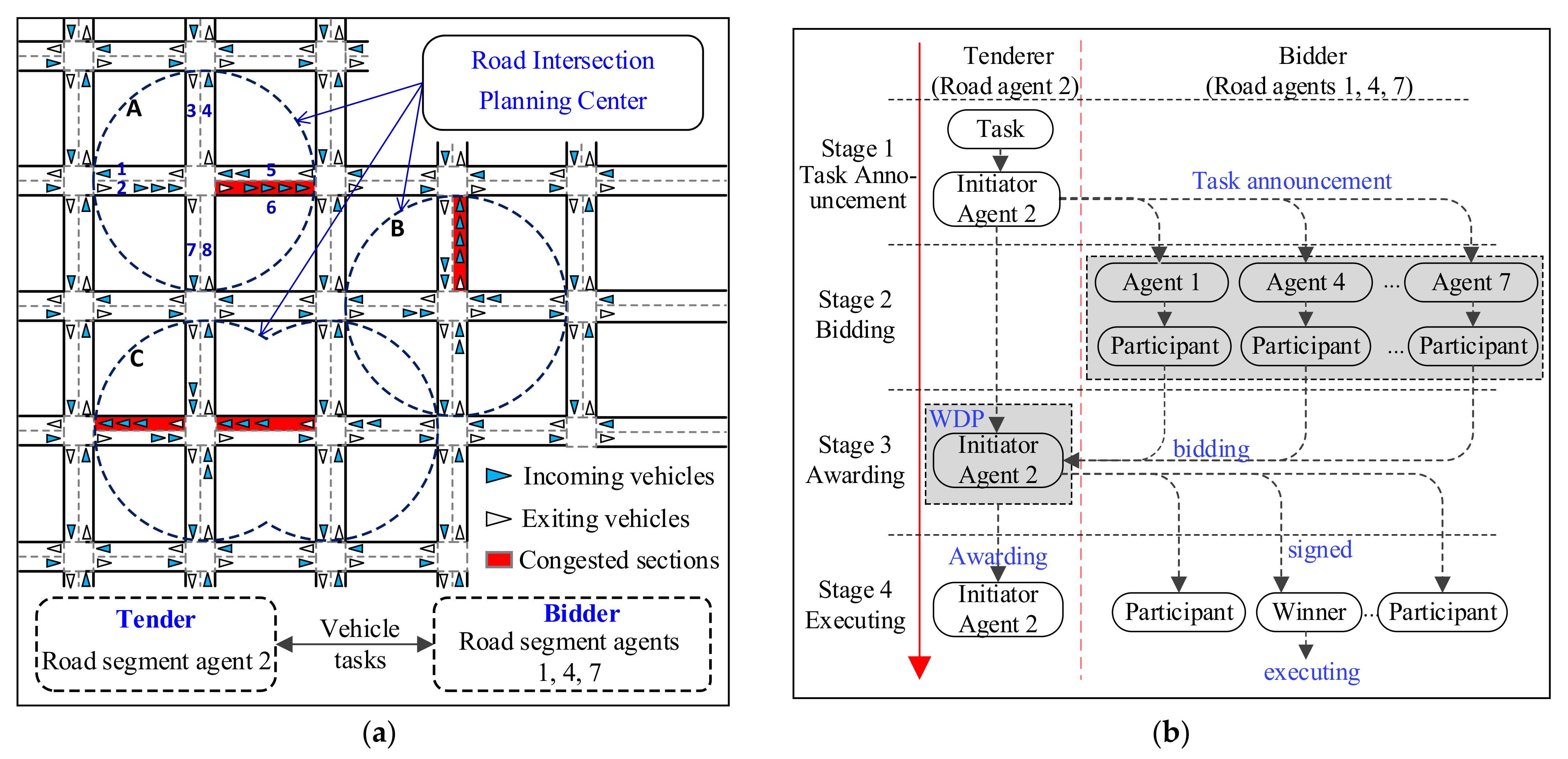
3.1. Bidding-Based Vehicle—Road Coordination Planning Method
| Algorithm 1 Bidding-based coordination planning algorithm |
| Input: |
| Set of vehicle tasks that requires route replanning |
| Road agents in R that require allocating vehicle tasks |
| Set of neighboring road agents of ri available for bidding |
| Output: |
| Vehicle task replanning scheme |
| 1 Let be a tenderer who publishes a bidding announcement to candidate bidders in RNi |
| 2 For each bidder in do |
| 3 Obtain the destinations of vehicles |
| 4 Calculate optimal paths and travel time from bidder to destinations for vehicles |
| 5 Determine the vehicle task set for bidding according to their planned vehicle tasks |
| 6 Submit bidding task replanning scheme and bidding price |
| 7 End |
| 8 Determine the set of winning bidding scheme by calling Algorithm 2 |
| 9 |
| 10 If then |
| 11 Return the replanning scheme |
| 12 Else |
| 13 Each vehicle in selects its optimal path independently |
| 14 Generate replanning scheme according to these paths |
| 15 Return the replanning scheme |
| 16 End if |
3.2. Winning Bidder Determination Algorithm
| Algorithm 2 Priority-set-based local search algorithm |
| Input: |
| S Set of bidding schemes submitted from all bidders |
| V Bidding price set |
| ρ Probability parameter within (0,1) |
| σ Bidding price interval parameter |
| Output: |
| Sbest Best vehicle task allocation scheme |
| 1 Initialize priority search schemes set = |
| 2 While changes in two adjacent iterations |
| 3 If then |
| 4 |
| 5 Else |
| 6 Temporary scheme set |
| 7 With probability do |
| 8 Determine the minimal price of bidding schemes in TemB |
| 9 Select bidding scheme set from within the floating price interval . |
| 10 Select scheme randomly from |
| 11 Otherwise |
| 12 Select t scheme randomly from |
| 13 Done |
| 14 |
| 15 Update : Remove bidding scheme that conflicts with from |
| 16 End if |
| 17 If the total price of is smaller than that of then |
| 18 |
| 19 End if |
| 20 Update PB according to the conflict relationship between and . |
| 21 End while |
| 22 Return |
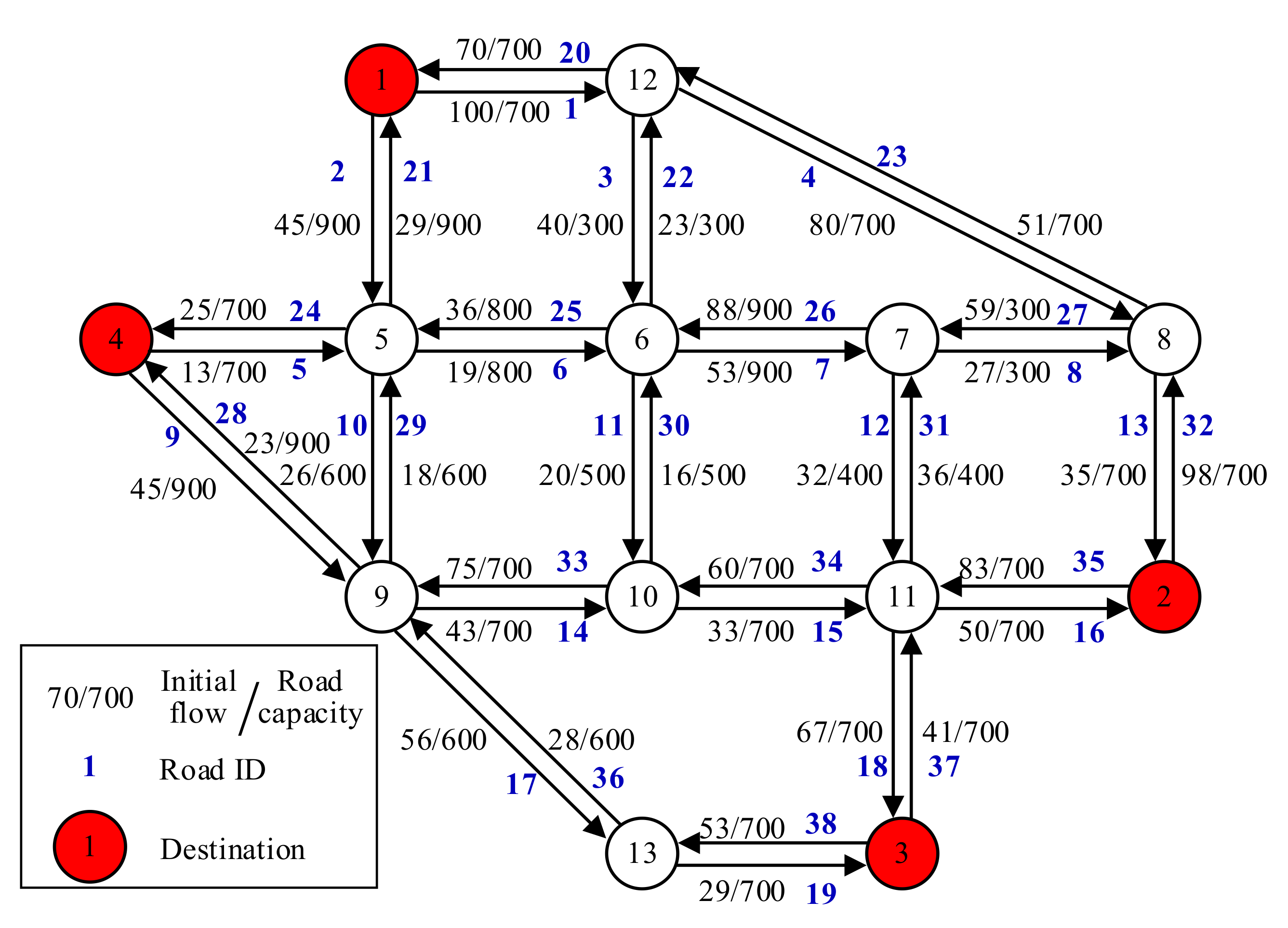
4. Case Study
4.1. Simulation Case Experiment
4.1.1. Experimental Setting
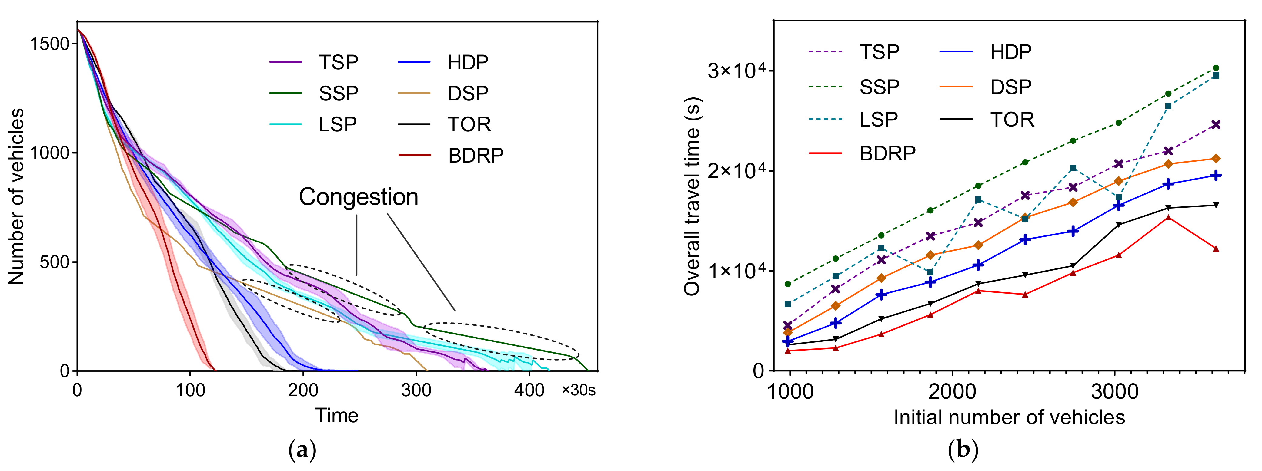
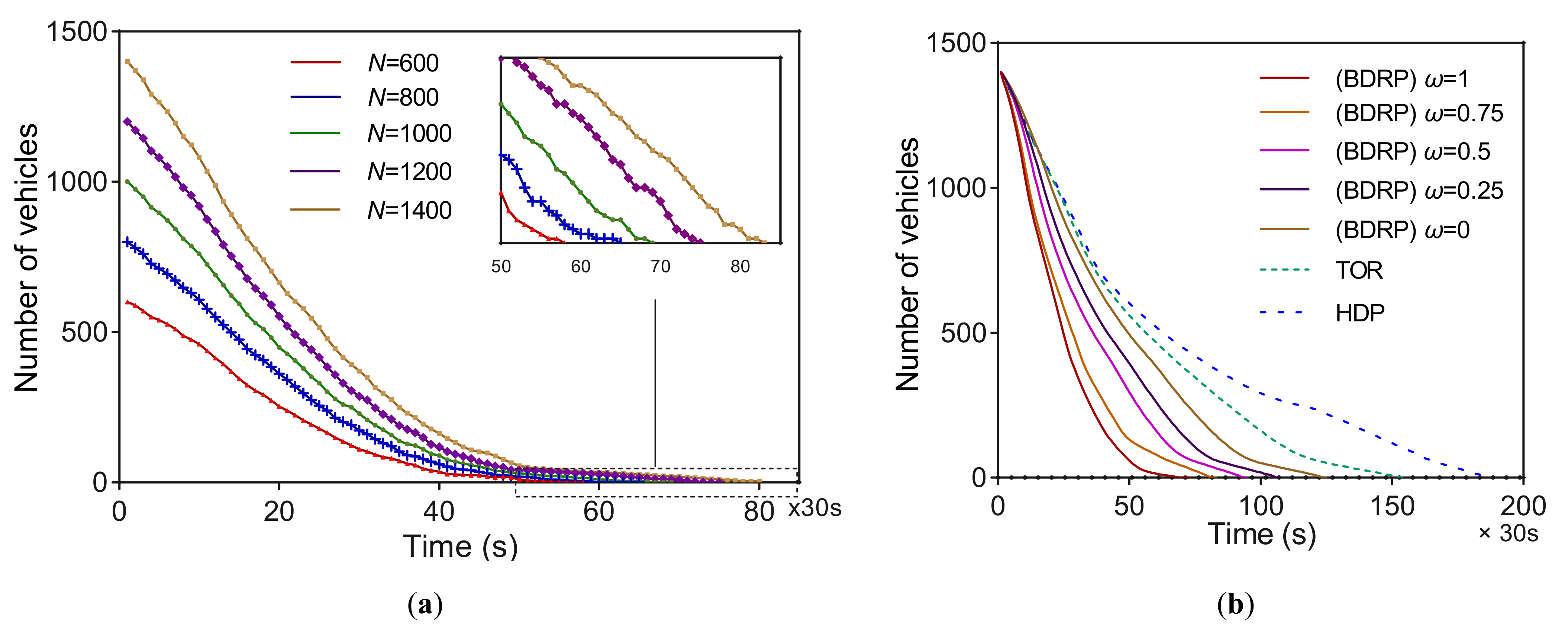
4.1.2. Network Transport Efficiency Comparison between Different Routing Schemes
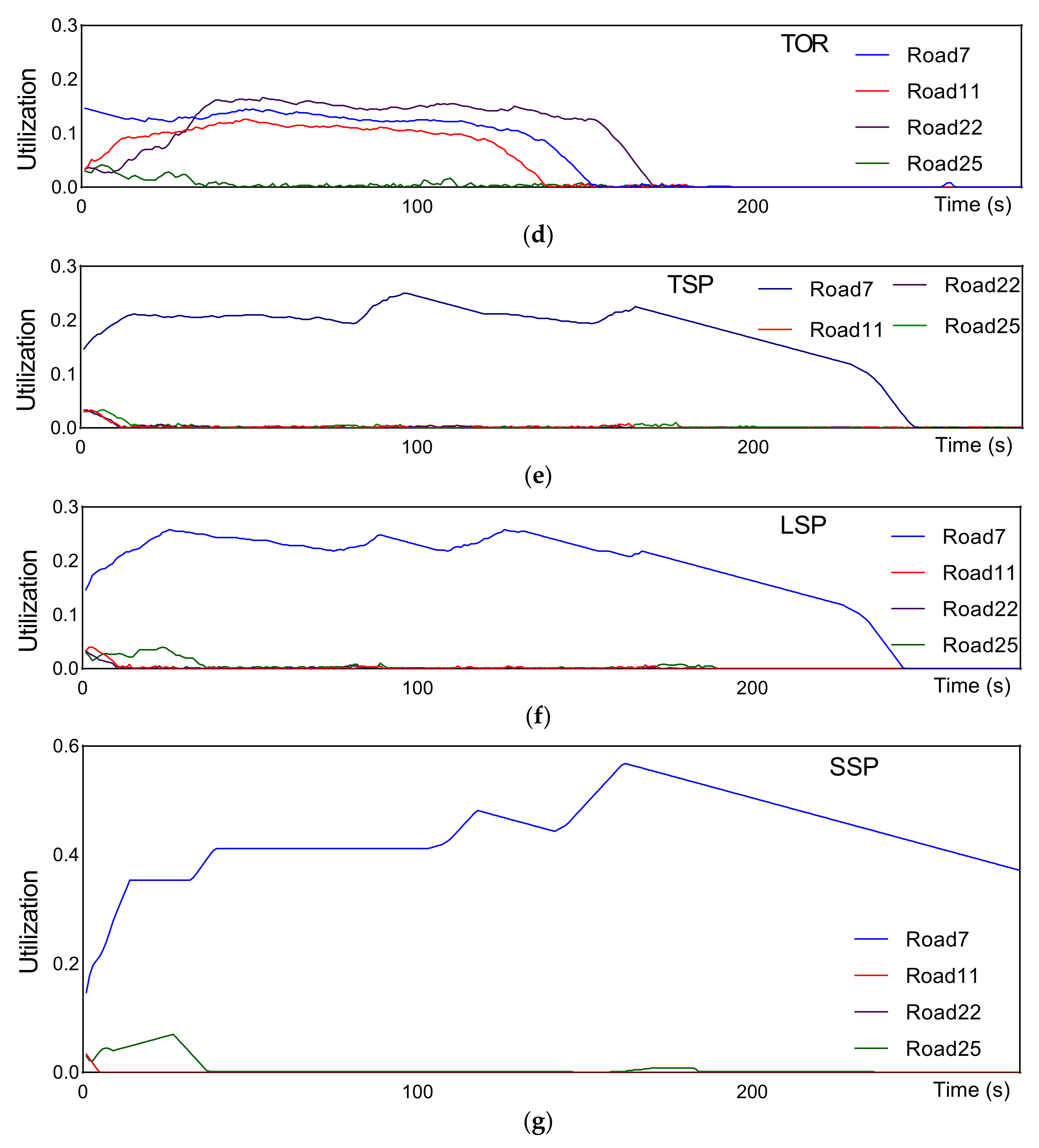
4.1.3. Road Utilization Rate Comparison between Different Methods
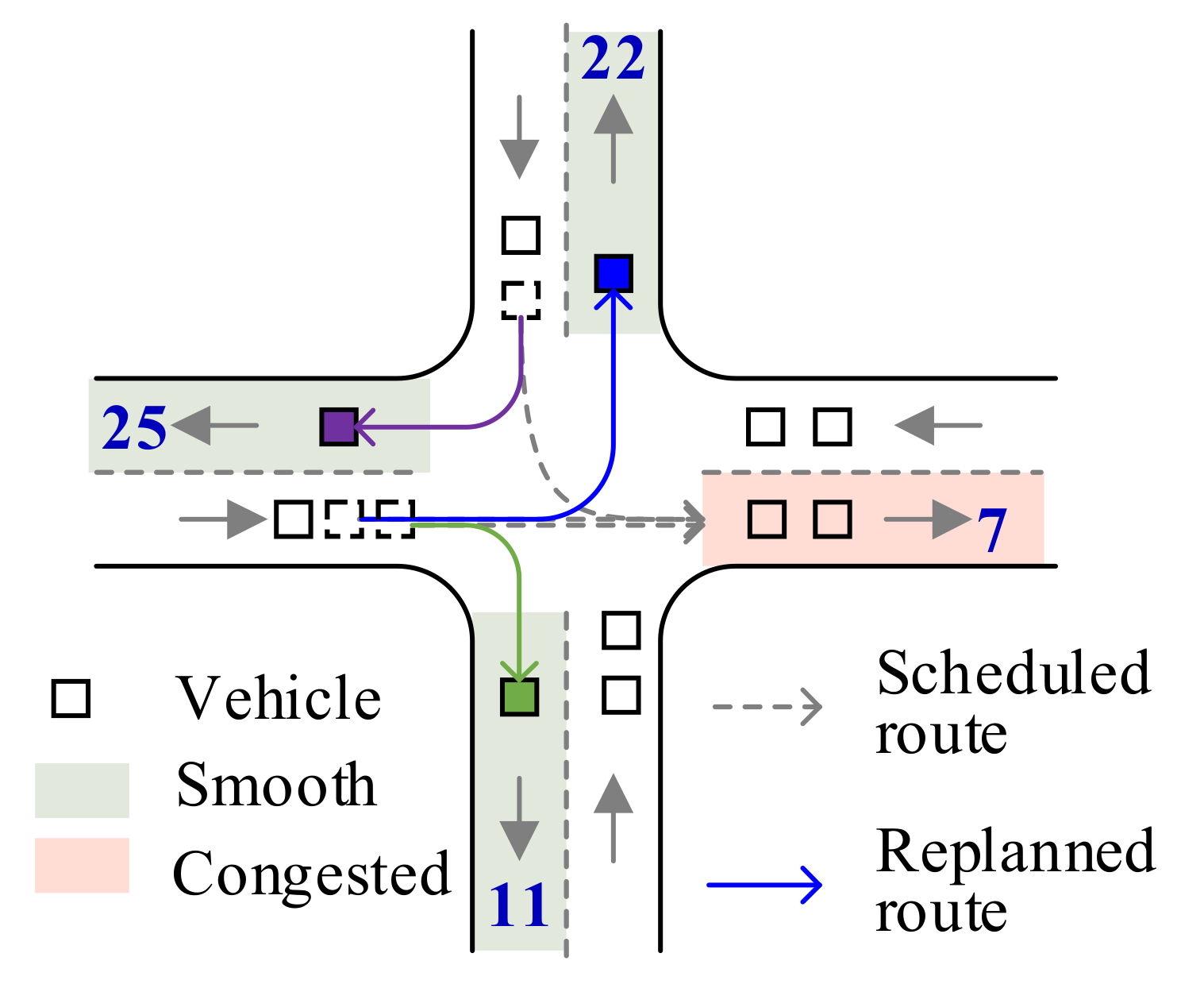
4.2. Example Application
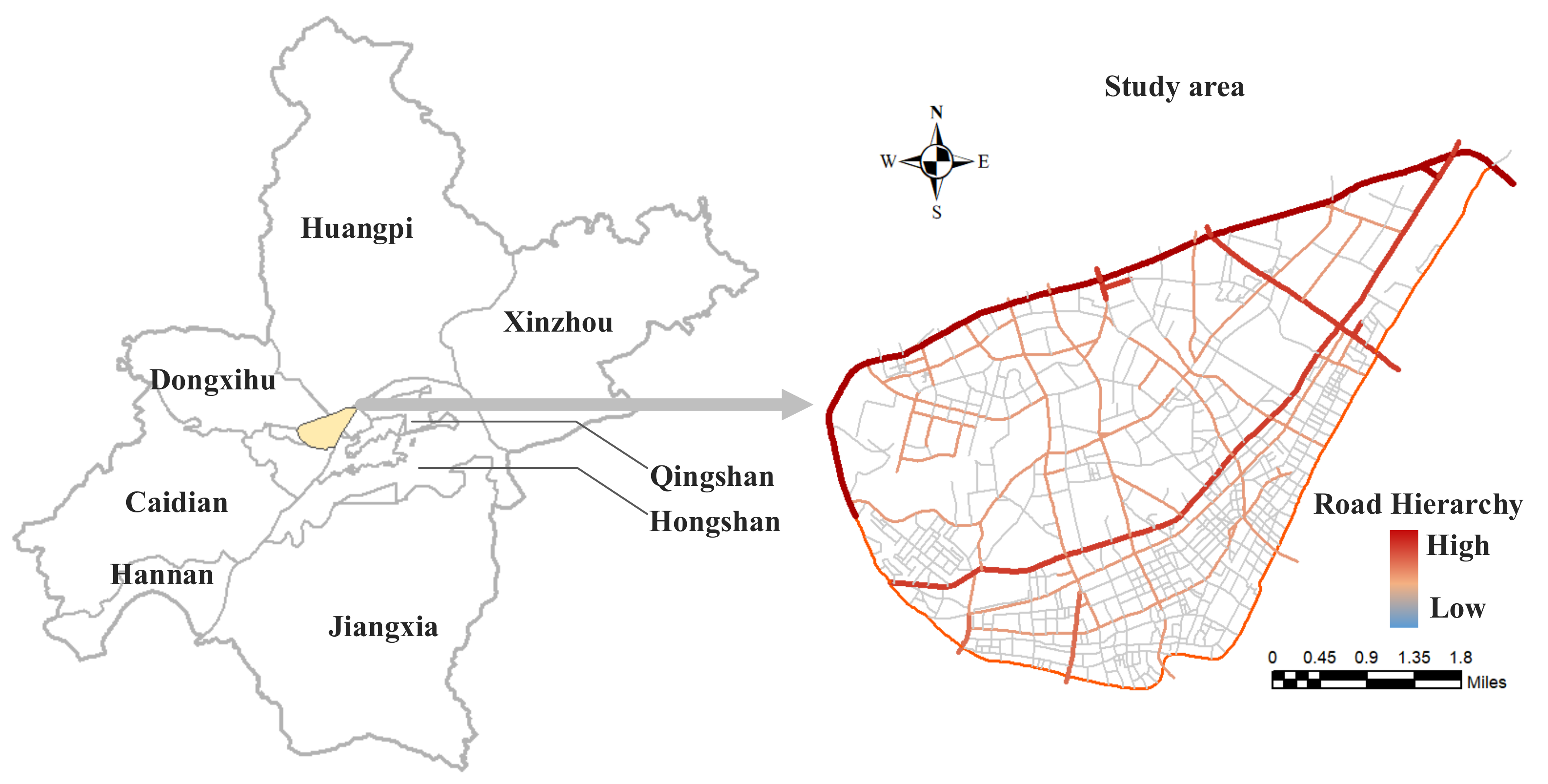
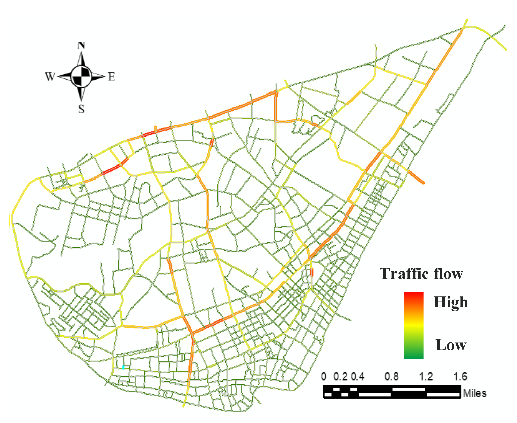
4.2.1. Study Area Description
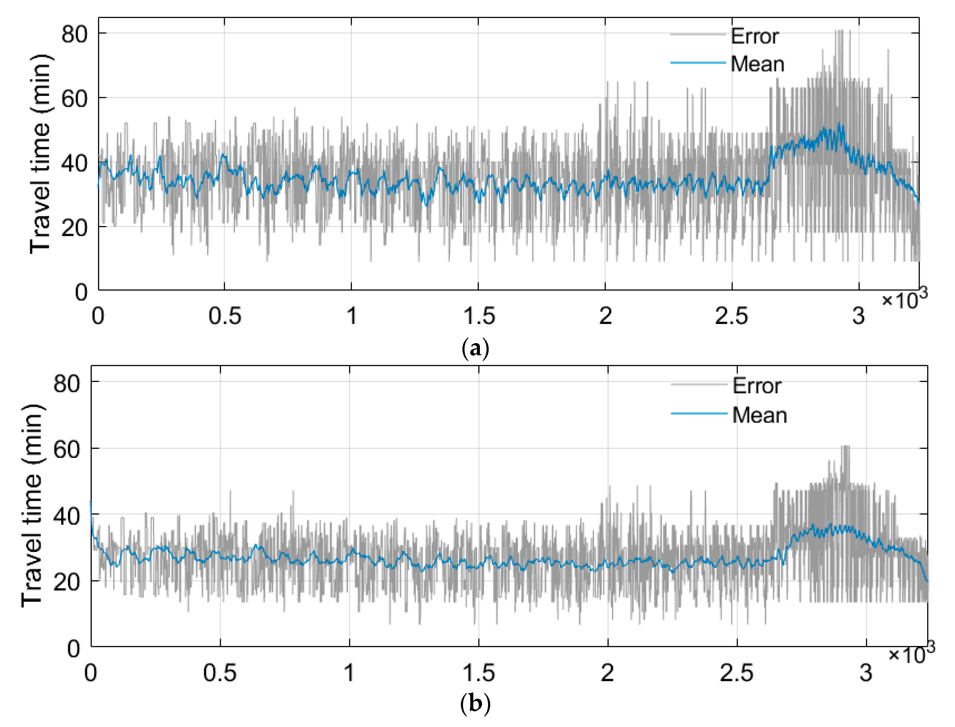
4.2.2. Transport Efficiency of the Road Network
5. Discussion
6. Conclusions
Author Contributions
Funding
Institutional Review Board Statement
Informed Consent Statement
Data Availability Statement
Acknowledgments
Conflicts of Interest
Abbreviations
| BDRP | bidding-based dynamic route planning |
| CV | connected vehicles |
| FIFO | first-in-first-out |
| BPR | Bureau of Public Roads |
| WDP | winner determination problem |
| PLS | priority-set-based local search |
| SSP | static shortest path method |
| TSP | top-K shortest path method |
| LSP | logit model-based shortest path method |
| HDP | hierarchical dynamic planning |
| TOR | time-optimization routing |
References
- Fan, S.; Chan-Kang, C. Regional road development, rural and urban poverty: Evidence from China. Transp. Policy 2008, 15, 305–314. [Google Scholar] [CrossRef]
- Liu, B.; Deng, M.; Yang, J.; Shi, Y.; Huang, J.; Li, C.; Qiu, B. Detecting anomalous spatial interaction patterns by maximizing urban population carrying capacity. Comput. Environ. Urban Syst. 2021, 87, 101616. [Google Scholar] [CrossRef]
- Ackaah, W. Exploring the use of advanced traffic information system to manage traffic congestion in developing countries. Sci. Afr. 2019, 4, e00079. [Google Scholar] [CrossRef]
- Sun, R.; Hu, J.; Xie, X.; Zhang, Z. Variable Speed Limit Design to Relieve Traffic Congestion based on Cooperative Vehicle Infrastructure System. Procedia Soc. Behav. Sci. 2014, 138, 427–438. [Google Scholar] [CrossRef] [Green Version]
- Liu, B.; Long, J.; Deng, M.; Tang, J.; Huang, J. Revealing spatiotemporal correlation of urban roads via traffic perturbation simulation. Sustain. Cities Soc. 2021, 103545. [Google Scholar] [CrossRef]
- Dijkstra, E.W. A note on two problems in connexion with graphs. Numer. Math. 1959, 1, 269–271. [Google Scholar] [CrossRef] [Green Version]
- Hart, P.E.; Nilsson, N.J.; Raphael, B. A Formal Basis for the Heuristic Determination of Minimum Cost Paths. IEEE Trans. Syst. Sci. Cybern. 1968, 4, 100–107. [Google Scholar] [CrossRef]
- Bellman, R. On a routing problem. Q. Appl. Math. 1958, 16, 87–90. [Google Scholar] [CrossRef] [Green Version]
- George, B.D. Linear Programming and Extensions; Princeton University Press: Princeton, NJ, USA, 1962. [Google Scholar]
- Geisberger, R.; Sanders, P.; Schultes, D.; Vetter, C. Exact Routing in Large Road Networks Using Contraction Hierarchies. Transp. Sci. 2012, 46, 388–404. [Google Scholar] [CrossRef]
- Delling, D.; Goldberg, A.V.; Razenshteyn, I.; Werneck, R.F. Graph partitioning with natural cuts. In Proceedings of the 25th International Parallel and Distributed Processing Symposium (IPDPS 2011), Anchorage, AK, USA, 16–20 May 2011; IEEE Computer Society: Washington, DC, USA, 2011; pp. 1135–1146. [Google Scholar]
- Delling, D.; Goldberg, A.V.; Werneck, R.F. Faster batched shortest paths in road networks. In Proceedings of the 11th Workshop on Algorithmic Approaches for Transportation Modeling, Optimization, and Systems (ATMOS 2011), OpenAccess Series in Informatics (OASIcs), Saarbrücken, Germany, 8 September 2011; Volume 20, pp. 52–63. [Google Scholar]
- Liu, G.; Long, W.; Wang, J.; Gao, P.; He, J.; Luo, Z.; Li, L.; Li, Y. Improving the throughput of transportation networks with a time-optimization routing strategy. Int. J. Geogr. Inf. Sci. 2018, 32, 1815–1836. [Google Scholar] [CrossRef]
- Xu, B.; Zhou, X. Dynamic relative robust shortest path problem. Comput. Ind. Eng. 2020, 148, 106651. [Google Scholar] [CrossRef]
- Xu, B.; Li, S.E.; Bian, Y.; Li, S.; Ban, X.J.; Wang, J.; Li, K. Distributed conflict-free cooperation for multiple connected vehicles at unsignalized intersections. Transp. Res. Part C Emerg. Technol. 2018, 93, 322–334. [Google Scholar] [CrossRef]
- Li, S.E.; Wang, Z.; Zheng, Y.; Sun, Q.; Gao, J.; Ma, F.; Li, K. Synchronous and asynchronous parallel computation for large-scale optimal control of connected vehicles. Transp. Res. Part C Emerg. Technol. 2020, 121, 102842. [Google Scholar] [CrossRef]
- Dai, R.; Lu, Y.; Ding, C.; Lu, G.; Wang, Y. A simulation-based approach to investigate the driver route choice behavior under the connected vehi-cle environment. Transp. Res. Part F Traffic Psychol. Behav. 2019, 65, 548–563. [Google Scholar] [CrossRef]
- Liu, Y.; Yu, Y. Distributed dynamic traffic modeling and implementation oriented different levels of induced travelers, Dis-crete Dyn. Nat. Soc. 2015, 2015, 642389. [Google Scholar]
- Zeng, W.; Miwa, T.; Wakita, Y.; Morikawa, T. Application of Lagrangian relaxation approach to α -reliable path finding in stochastic networks with correlated link travel times. Transp. Res. Part C Emerg. Technol. 2015, 56, 309–334. [Google Scholar] [CrossRef]
- Lei, F.; Wang, Y.; Lu, G.; Sun, J. A travel time reliability model of urban expressways with varying levels of service. Transp. Res. Part C Emerg. Technol. 2014, 48, 453–467. [Google Scholar] [CrossRef]
- Lee, S.; Heydecker, B.G.; Kim, J.; Park, S. Stability analysis on a dynamical model of route choice in a connected vehicle environment. Transp. Res. Procedia 2017, 23, 720–737. [Google Scholar] [CrossRef]
- Jamson, S.L.; Brouwer, R.; Seewald, P. Supporting Eco-Driving. Transp. Res. Part C Emerg. Technol. 2015, 58, 629–630. [Google Scholar] [CrossRef]
- Genders, W.; Razavi, S.N. Impact of Connected Vehicle on Work Zone Network Safety through Dynamic Route Guidance. J. Comput. Civ. Eng. 2016, 30, 04015020. [Google Scholar] [CrossRef]
- Roughgarden, T.; Tardos, É. How bad is selfish routing? JACM 2002, 49, 236–259. [Google Scholar] [CrossRef]
- Lazar, D.A.; Bıyık, E.; Sadigh, D.; Pedarsani, R. Learning how to dynamically route autonomous vehicles on shared roads. Transp. Res. Part C Emerg. Technol. 2021, 130, 103258. [Google Scholar] [CrossRef]
- Youn, H.; Gastner, M.T.; Jeong, H. Price of anarchy in transportation networks: Efficiency and opti-mality control. Phys. Rev. Lett. 2008, 101, 128701. [Google Scholar] [CrossRef] [PubMed] [Green Version]
- Yildirimoglu, M.; Ramezani, M.; Geroliminis, N. Equilibrium Analysis and Route Guidance in Large-scale Networks with MFD Dynamics. Transp. Res. Procedia 2015, 9, 185–204. [Google Scholar] [CrossRef] [Green Version]
- Shi, Y.; Wang, D.; Tang, J.; Deng, M.; Liu, H.; Liu, B. Detecting spatiotemporal extents of traffic congestion: A density-based moving object clustering approach. Int. J. Geogr. Inf. Sci. 2021, 35, 1449–1473. [Google Scholar] [CrossRef]
- Çolak, S.; Lima, A.; González, M.C. Understanding congested travel in urban areas. Nat. Commun. 2016, 7, 1–8. [Google Scholar] [CrossRef]
- Liang, L.; Yang, Y.; Wang, H.; Huang, L.; Zhang, X. Traffic Impedance Estimation Driven by Trajectories for Urban Roads. In Proceedings of the 3rd International Conference on Vision, Image and Signal Processing, Vancouver, BC, Canada, 26–28 August 2019; pp. 1–7. [Google Scholar] [CrossRef]
- Nguyen, S.; Dupuis, C. An Efficient Method for Computing Traffic Equilibria in Networks with Asymmetric Transportation Costs. Transp. Sci. 1984, 18, 185–202. [Google Scholar] [CrossRef]
- Chen, B.Y.; Lam, W.H.; Sumalee, A.; Li, Z.L. Reliable shortest path finding in stochastic networks with spatial correlated link travel times. Int. J. Geogr. Inf. Sci. 2012, 26, 365–386. [Google Scholar] [CrossRef]
- Woelki, M.; Lu, T.; Ruppe, S. Ranking of alternatives for emergency routing on urban road networks. WIT Trans. Built Environ. 2015, 146, 591–598. [Google Scholar] [CrossRef] [Green Version]
- KuKuijpers, B.; Moelans, B.; Othman, W.; Vaisman, A. Uncertainty-based map matching: The space time prism and k-shortest path algo-rithm. ISPRS Int. J. Geo Inf. 2016, 5, 204. [Google Scholar] [CrossRef] [Green Version]
- Liu, Z.; Wang, S.; Meng, Q. Toll pricing framework under logit-based stochastic user equilibrium constraints. J. Adv. Transp. 2013, 48, 1121–1137. [Google Scholar] [CrossRef] [Green Version]
- Wang, J.; Niu, H. A distributed dynamic route guidance approach based on short-term forecasts in cooperative infrastruc-ture-vehicle systems. Transp. Res. Part D Transp. Environ. 2019, 66, 23–34. [Google Scholar] [CrossRef]
- Sunita; Garg, D. Dynamizing Dijkstra: A solution to dynamic shortest path problem through retroactive priority queue. J. King Saud Univ. Comput. Inf. Sci. 2021, 33, 364–373. [Google Scholar] [CrossRef]
- Wang, P.; Deng, H.; Zhang, J.; Zhang, M. Realtime urban regional route planning model for connected vehicles based on V2X communication. J. Transp. Land Use 2020, 13, 517–538. [Google Scholar] [CrossRef]


| Parameter | Value |
|---|---|
| Number of nodes in the network | 13 |
| Number of road segments in the network | 38 |
| Traffic density during congestion ρjam (N/L) | 0.15 |
| Time step (s) | 30 |
| Road hierarchy | {1,2,3,4} |
| Road design speed (km/h) | {70,50,35,25} |
| ω in Equation (3) | 0.5 |
| α in Equation (4) | 0.28 |
| β in Equation (4) | 2.35 |
| Initial Number of Vehicles | Method | ||||||
|---|---|---|---|---|---|---|---|
| TSP | SSP | LSP | HDP | DSP | BDRP | TOR | |
| 986 | 5.49 | 0.99 | 5.47 | 7.39 | 39.29 | 13.43 | 138.34 |
| 1281 | 6.03 | 1.06 | 6.35 | 14.14 | 74.16 | 25.51 | 254.99 |
| 1562 | 7.12 | 1.26 | 7.61 | 29 | 111.62 | 45.35 | 405.82 |
| 1865 | 8.89 | 1.56 | 9.59 | 32.93 | 206.3 | 78.09 | 626.19 |
| 2160 | 9.43 | 1.75 | 9.83 | 48.41 | 307.91 | 82.52 | 818.87 |
| 2448 | 11.48 | 2.16 | 11.35 | 56.93 | 396.29 | 129.56 | 1081.06 |
| 2743 | 12.36 | 2.3 | 13.05 | 85.49 | 535.68 | 147.1 | 1391.14 |
| 3024 | 15.15 | 2.59 | 13.85 | 86.89 | 739.07 | 197.36 | 1817.88 |
| 3330 | 16.11 | 3.03 | 16.76 | 115.46 | 1107.26 | 223.05 | 2249.37 |
| 3622 | 16.19 | 3.21 | 18.85 | 127.62 | 1592.05 | 255.59 | 2826.71 |
| Parameter | Value |
|---|---|
| Number of nodes in the network | 1062 |
| Number of road segments in the network | 1596 |
| Traffic density during congestion (N/L) | 0.15 |
| Time step (s) | 30 |
| Road hierarchy | {1,2,3,4} |
| Road design speed (km/h) | {70,50,35,25} |
| in Equation (4) | 0.28 |
| in Equation (4) | 2.35 |
Publisher’s Note: MDPI stays neutral with regard to jurisdictional claims in published maps and institutional affiliations. |
© 2022 by the authors. Licensee MDPI, Basel, Switzerland. This article is an open access article distributed under the terms and conditions of the Creative Commons Attribution (CC BY) license (https://creativecommons.org/licenses/by/4.0/).
Share and Cite
Liu, B.; Long, J.; Deng, M.; Yang, X.; Shi, Y. An Adaptive Route Planning Method of Connected Vehicles for Improving the Transport Efficiency. ISPRS Int. J. Geo-Inf. 2022, 11, 39. https://doi.org/10.3390/ijgi11010039
Liu B, Long J, Deng M, Yang X, Shi Y. An Adaptive Route Planning Method of Connected Vehicles for Improving the Transport Efficiency. ISPRS International Journal of Geo-Information. 2022; 11(1):39. https://doi.org/10.3390/ijgi11010039
Chicago/Turabian StyleLiu, Baoju, Jun Long, Min Deng, Xuexi Yang, and Yan Shi. 2022. "An Adaptive Route Planning Method of Connected Vehicles for Improving the Transport Efficiency" ISPRS International Journal of Geo-Information 11, no. 1: 39. https://doi.org/10.3390/ijgi11010039
APA StyleLiu, B., Long, J., Deng, M., Yang, X., & Shi, Y. (2022). An Adaptive Route Planning Method of Connected Vehicles for Improving the Transport Efficiency. ISPRS International Journal of Geo-Information, 11(1), 39. https://doi.org/10.3390/ijgi11010039