Potential Use of Drone Ultra-High-Definition Videos for Detailed 3D City Modeling

Abstract

Ongoing developments in video resolution either using consumer-grade or professional cameras has opened opportunities for different applications such as in sports events broadcasting and digital cinematography. In the field of geoinformation science and photogrammetry, image-based 3D city modeling is expected to benefit from this technology development. Highly detailed 3D point clouds with low noise are expected to be produced when using ultra high definition UHD videos (e.g., 4K, 8K). Furthermore, a greater benefit is expected when the UHD videos are captured from the air by consumer-grade or professional drones. To the best of our knowledge, no studies have been published to quantify the expected outputs when using UHD cameras in terms of 3D modeling and point cloud density. In this paper, a quantification is shown about the expected point clouds and orthophotos qualities when using UHD videos from consumer-grade drones and a review of which applications they can be applied in. The results show that an improvement in 3D models of ≅65% relative accuracy and ≅90% in point density can be attained when using 8K video frames compared with HD video frames which will open a wide range of applications and business cases in the near future.

1. Introduction

Currently, most consumer-grade drones (unmanned aerial vehicles, UAVs) are equipped with a camera capable of capturing HD videos of 1920 × 1280 pixels (2K). As shown in different research articles, this image resolution enables the creation of 3D models of degraded quality that is more suitable for virtual reality or virtual tourism but still not enough for 3D documentation applications [1]. Accordingly, this research is aimed to answer the following question: what is the improvement in the derived 3D models we can gain if a drone is equipped with an ultra-high definition UHD 6K and 8K video resolution camera?

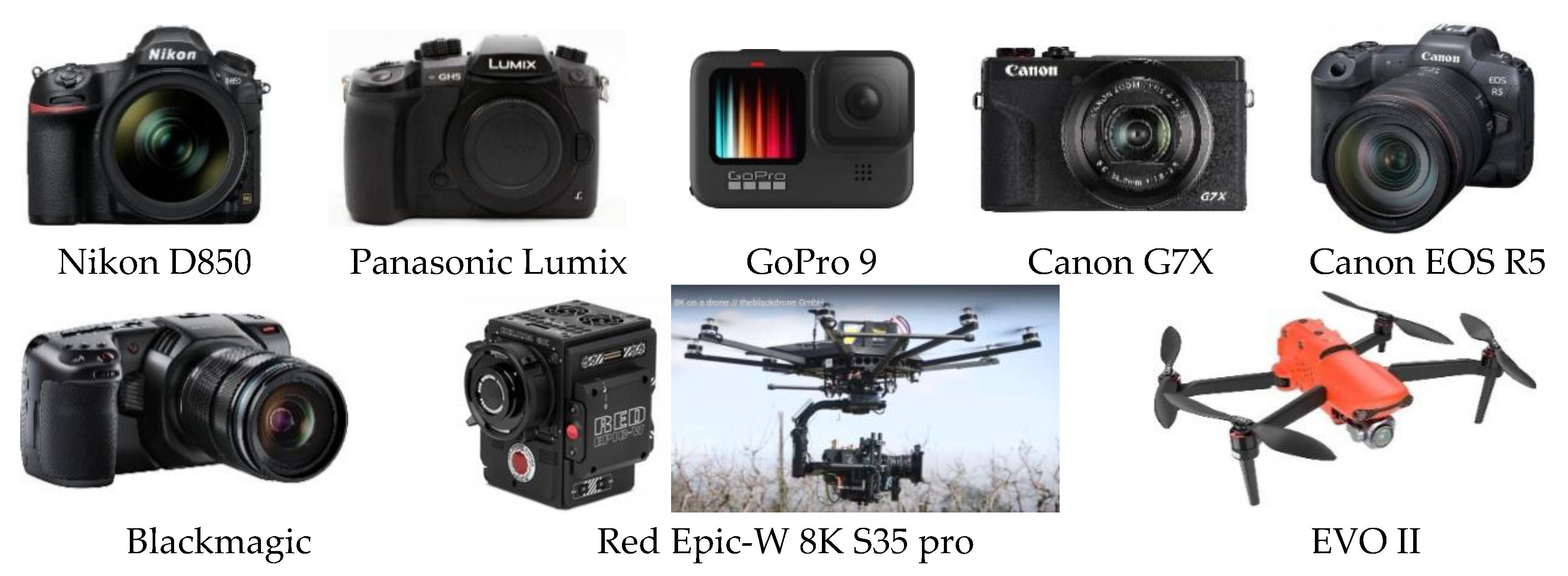
Increasingly, the 4K cameras either professional or compact are mounted on the drones to offer the customer high-resolution images with higher quality and details. As an example, DJI [2] and Skydio [3] are equipped with 4K cameras. Examples of current 4K cameras are Panasonic Lumix DMC-GH5 [4], Nikon D850, Canon PowerShot G7X [5], Canon EOS R5 [6], and GoPro 9 Black 4K @ 60 fps 5K@30 fps [7] (Figure 1).

Few researchers have shown the use of 4K videos for 3D modeling applications such as in [1] and still, no research has shown the comparison between the quality of the 3D models when using drone HD videos compared with 4K videos or UHD.

On the other hand, 6K and 8K video resolution cameras are starting to be found in the market but on the professional camera level and are expected to popularize 6K and 8K consumer-grade cameras in the near future. As an example of the UHD cameras, the Blackmagic Pocket Cinema camera has a 6K video image resolution of 6144 × 3456 at 60 fps [2] (Figure 1). Increasingly, consumer-grade drones will be equipped with these UHD cameras and this motivates us to introduce this research to quantify the benefit expected when using such UHD video cameras mounted on drones in terms of the quality of the created 3D models and orthophotos.

Noticeably, the UHD video imaging resolutions (e.g., 4K, 6K, and 8K) have several benefits because they show less noise due to bigger sensor size, are effective for low light conditions, have realistic image quality, capture more details, etc. [3].

8K video frame resolution is currently the highest in the industry of digital television and digital cinematography. As it implies from its name, it is equivalent to two times the resolution (pixels) of 4K images and sixteen times the number of pixels of HD images. This means that it is possible to capture recordings from a farther distance while maintaining the same imaging scale with high-quality results. Currently, few companies produced cameras capable of 8K resolution video capturing (8192 × 4320 pixels) which will have a great improvement in the imaging world and filmmaking [4]. The technical challenge to capture 8K videos is the large memory it needs, for example, 40 min of footage can consume up to 2 terabytes of storage memory [5]. Still, having an 8K camera onboard a drone is unreachable due to the high cost of such cameras and the memory required. Big companies such as Canon and Nikon are working on releasing their first 8k video-capable cameras but are still under development. Filmmakers currently can use 8K high-end heavy cameras such as the RED Helium mounted on drones as shown in Figure 1. However, in a few years, low-cost 8K cameras will be available in the market and can then be mounted on consumer-grade drones. Lately, Autel Robotics released their EVO II drone with a camera capable of recording 8K video at 25 fps and 48 MP still shots [6] which is considered the first drone in the world to have this camera’s high-resolution ability.

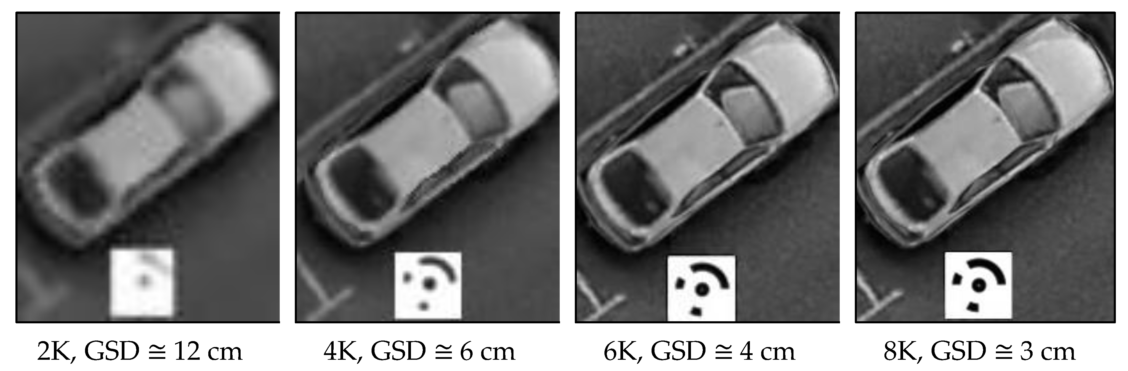
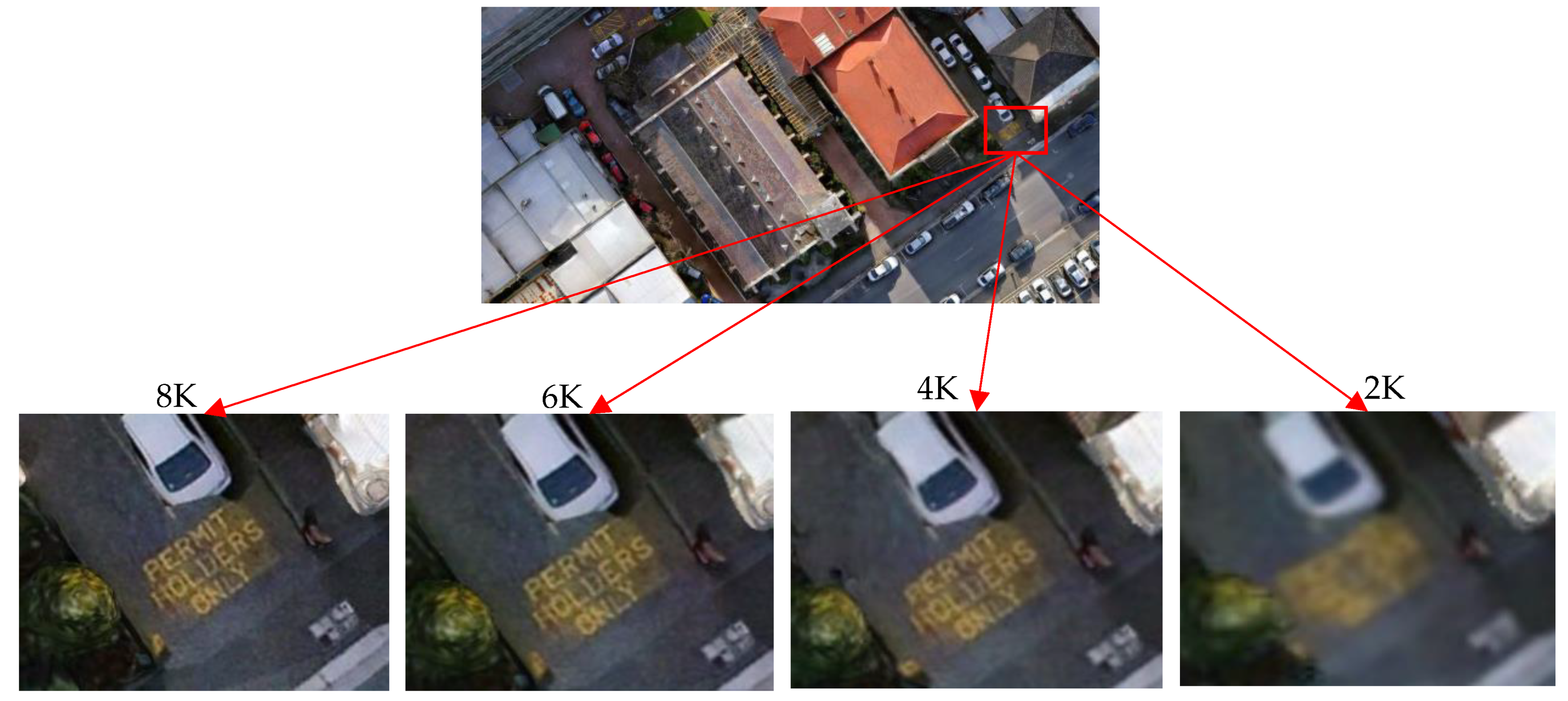
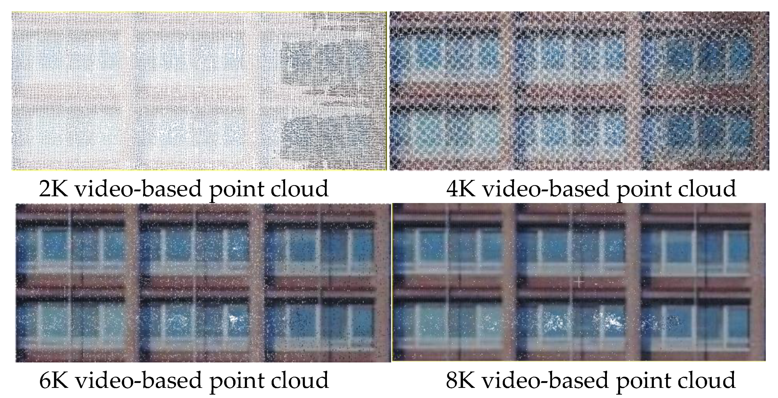
To illustrate the pictorial improvement gained when using UHD videos, two objects of a coded target of one squared meter and a nearby parked car are shown in Figure 2 graduating from HD (2K) to 8K. Worth mentioning is the ground sampling distance (GSD) at the 8K image resolution is improved four times compared with the 2K image resolution.

1.1. Video-Based 3D Modeling

Mostly, 3D image-based modeling is based on taking still shot images where an overlap percentage should be preserved. Research shows that 80% for both end lap and side lap is sufficient to create a 3D model and orthophotos out of the drone images [7,8]. This high overlap percentage implies a short baseline configuration which is preferred in the dense reconstruction [7,9].

On the other hand, 3D image-based models can be created using videos in what is sometimes called videogrammetry, which refers to making measurements from video images taken using a camcorder [10]. Basically, a video movie comprises a sequence of image frames captured at a certain recording speed. As an example, if a camera is used to capture a one-minute video at a speed of 30 frames per second (fps), it means that a total of 1800 video frames are recorded.

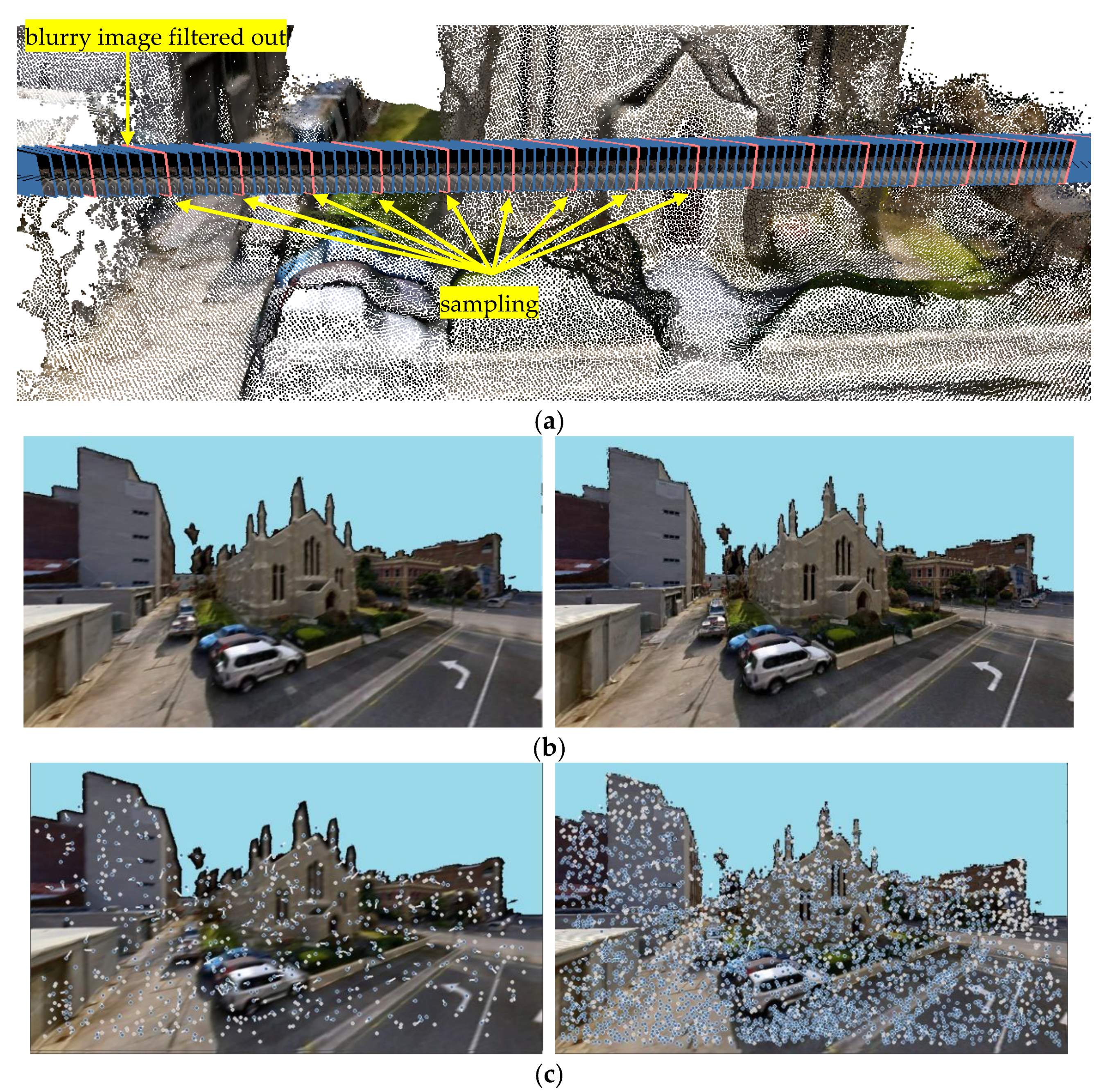
Video images represent a very short baseline imaging configuration where the point of correspondences between the video frames can be calculated by the so-called feature tracking like by using the Kanade–Lucas–Tomasi (KLT) method [11]. However, sampling the required frames can be applied either at fixed-time intervals (Figure 3a) or using more advanced methods such as the 2D features blurry image filtering [12]. In Figure 3b, two adjacent video frames are shown where one is blurred and one is sharp. In Figure 3c, the blurred image has a reduced number of SIFT keypoints [13] compared with the unblurred image. Filtering and sampling are logical to avoid the redundancy of the data, reduce the processing time, filter out the blurry images for a better 3D model [14], and have a geometrically stronger configuration.

Until now, video-based 3D modeling has not been preferred because of the insufficient resolution and very short baseline. As is known, a short baseline can lead to a small base/height (B/H) ratio which is unwanted because it implies a bad intersection angle and a large depth uncertainty compared with the wide baseline imaging configuration. As mentioned, sampling the video frames at longer time intervals can help to have a wider baseline configuration and decrease data redundancy.

Remarkably, taking videos is more flexible to record than still shots where the streaming continues to the target object without paying attention to the camera shutter speed, optimal waypoint along the flight trajectories, etc.

What can increase or popularize the use of video-based 3D modeling is the increase in the video resolution since the other technical details are already solved such as the structure from motion SfM or image matching, and most state-of-the-art software tools can process such data. Accordingly, UHD videos may replace static imagery as they gather the positive aspects of being high resolution, easy to capture and record, offer a wealth of data, and require less effort for planning. However, sampling and filtering are necessary to ensure cost-effective processing and good quality results. Currently, studies show that an accuracy of ≅1/400 or ≅5 cm can be achieved when using video frames of 640 × 480 pixels which can be improved to 1 cm with a higher resolution in the best case [14,15,16,17]. However, no studies have been applied to quantify the accuracies that can be achieved when capturing UHD videos ranging from 4K up to 8K. Accordingly, in this paper, a study will be conducted (Section 3) through two experiments using a drone equipped with a 2K, 4K, 6K, and 8K camera in a simulated environment.

1.2. UAV Flight Planning

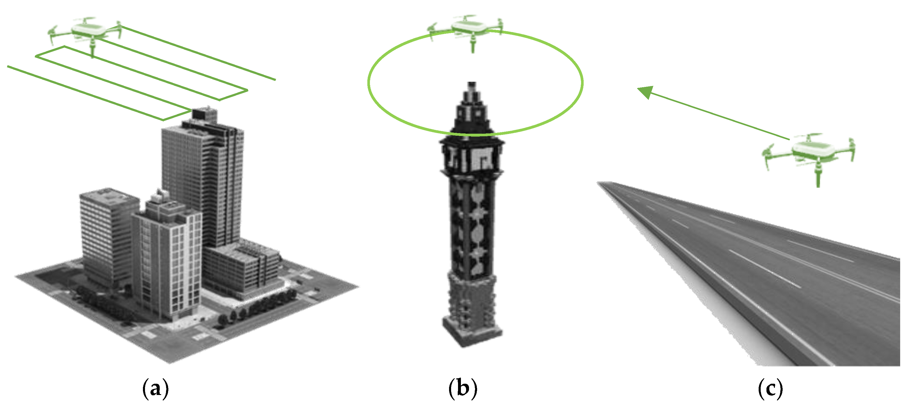
Flight planning is an important step to accomplish a successful UAV flight mission and achieve the mapping project goals and requirements. Several flight planning patterns can be applied depending on the task of the flight and the area of interest. For example, the flight plan for road and powerline mapping is different than the flight plans required for mapping an area of land or a tower. Accordingly, several flight plan patterns are found as shown in Figure 4.

To apply a flight plan [18,19], several imaging parameters should be selected. Overlap percentages between successive images and strips in the forward and side directions should be fixed. Camera parameters such as the focal length and flying height are used to set up a required scale and GSD. Camera shutter speed and the drone flying speed are also carefully set up to avoid imaging motion blur.

Worth mentioning is that more advanced flight planning is under continuous development and has started to be used to accomplish production of more autonomous drones where collision avoidance [20] and simultaneous localization and mapping (SLAM) [21,22] are applied. Skydio [23] and Anafi AI [24] are examples of such semi-autonomous consumer-grade drones currently available in the market.

2. Methodology

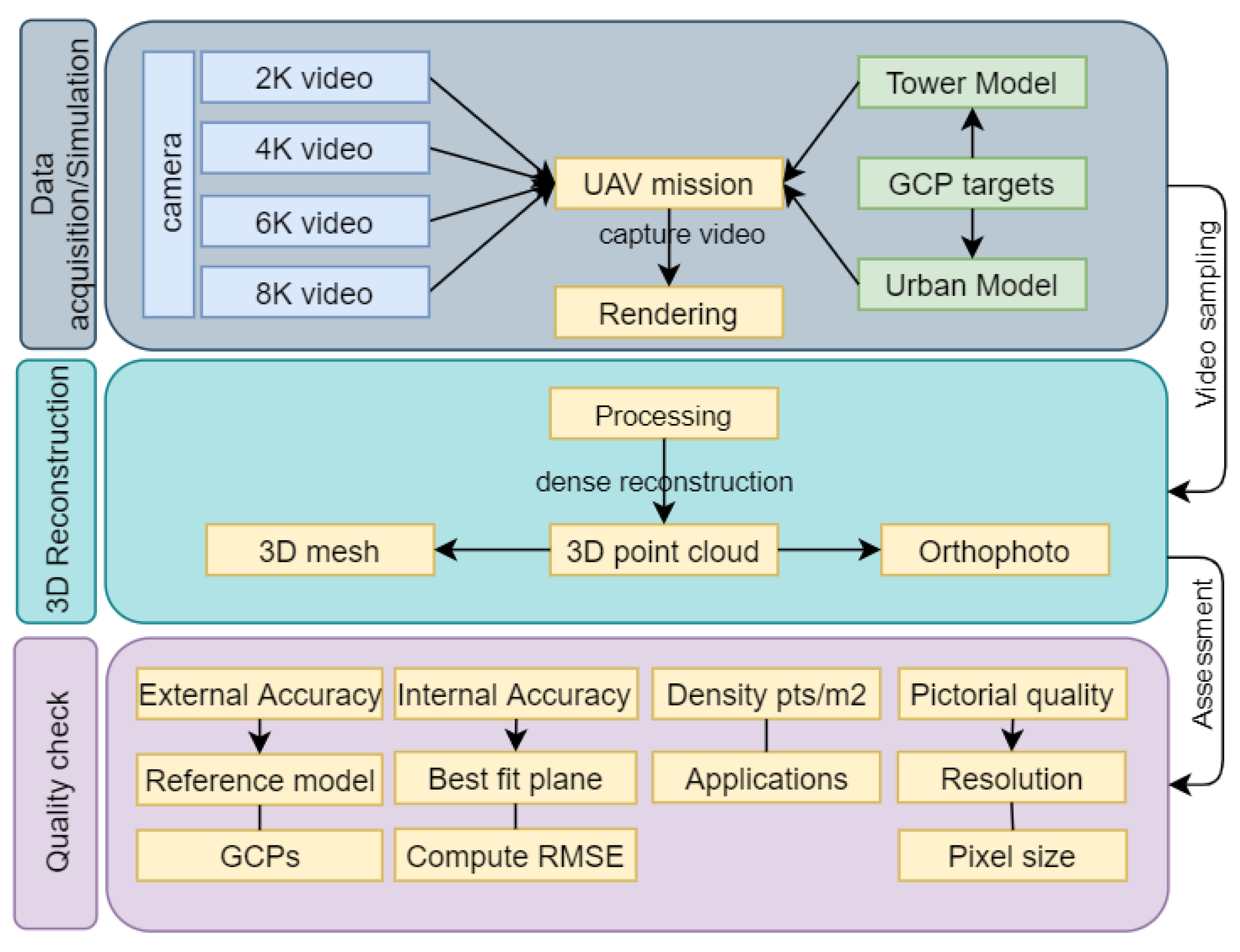
The methodology followed in this paper (Figure 5) uses a simulated environment using the Blender tool [25] where it is possible to test the four different video resolutions captured from the same drone at exactly the same flight trajectory. This is motivated by having a fair comparison between the produced models. Accordingly, two open-access 3D models are used: an urban scene [26] and a multi-story building [27] where a drone flight trajectory will be simulated. It is worth mentioning that ground control points (GCPs) will also be placed on the models represented by one squared-meter coded target. Then, after applying the drone missions, the video frames will be rendered and exported to the Metashape software tool [28] after sampling and filtering. Since the frames will be captured at a high rate of 20–30 frames/sec and as mentioned in Section 1, we will apply the frame sampling at fixed-time intervals to ensure the overlap percentage in the range of 80–90% for adequate 3D modeling. However, the blur effect will not be considered in the simulated video frames.

The designed GCPs fixed XYZ coordinates in both experiments will be assigned to the detected coded targets in the Metashape tool. Then, the image orientation will be applied using SfM. The dense reconstruction will be followed to create the point clouds and the point density will be estimated by counting the number of neighbors for each point inside a half-meter radius sphere using Cloud Compare [29].

To check the internal (relative) accuracy, planar patches out of the point clouds are extracted and the root mean squared error (RMSE) is calculated for every drone video capture. To continue the assessment, external (absolute) accuracy is investigated by calculating RMSE to GCPs and checkpoints.

Furthermore, the point cloud is turned into a surface mesh and finally, an orthomosaic is created. Then, the three results of the relative accuracy, density, and orthomosaic quality are evaluated for a final conclusion.

3. Results

Two experiments were applied in an urban environment using advanced simulations of the Blender tool. The four video frame resolutions of 2K, 4K, 6K, and 8K were tested in terms of point cloud density and relative accuracy. It is worth mentioning that both tests are applied using a laptop Dell Intel Core i7-9750H, CPU @ 2.60GHz, GPU Intel UHD Graphics 630 with 16 GB RAM.

1st experiment: urban model.

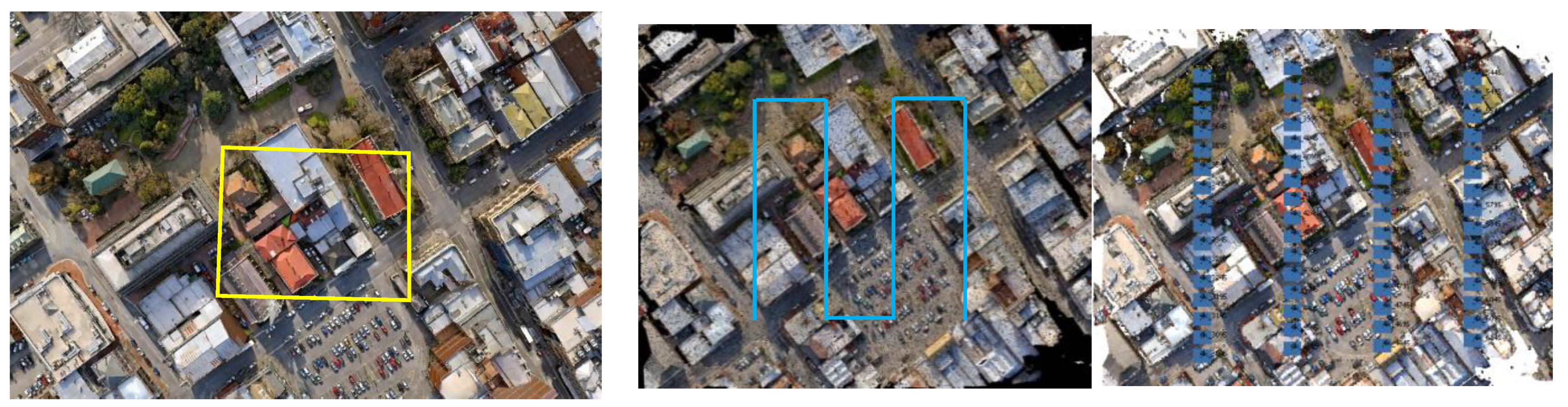
The first experiment is applied in an urban environment of Launceston city using its freely published model [26] where a flight plan is simulated assuming four different video resolutions as mentioned. The flight plan is selected in a grid trajectory (Figure 4a) around the area of interest (Figure 6).

The flight plan is applied using the following flight parameters:

Focal length = 2.77 mm

Pixel size = 1.6 µm

Sensor dimensions =6.16 × 4.6 mm

Flying height = 80 m

Forward overlap = 60% and side overlap = 40%

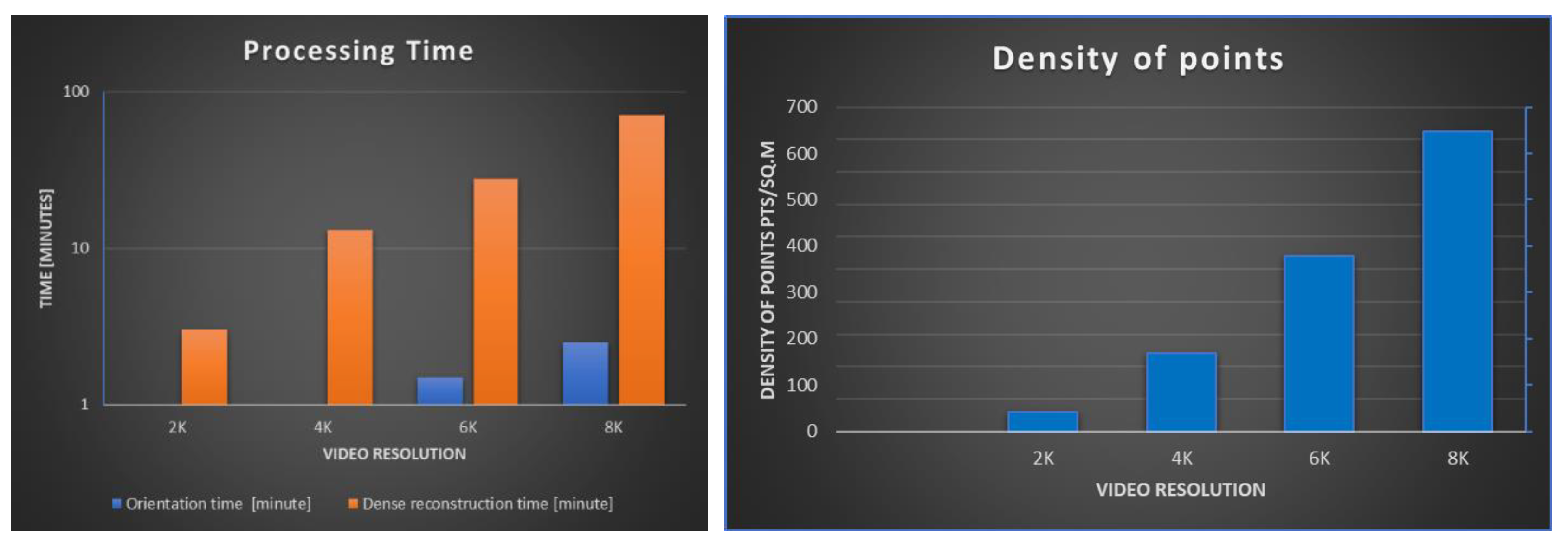
As mentioned, the simulations are applied using the Blender tool and the images of every video resolution are rendered at the same designed flight path at 80 m average height and assuming a recording speed of 20 frames per second. The video frames are sampled at regular intervals to end up with 63 video frames and ensure an 80% overlap.

The four video resolutions are processed using the Metashape tool and a dense point cloud is acquired at every image resolution. Figure 7 shows two histograms of the relation between the video resolution and the time consumption and density of points.

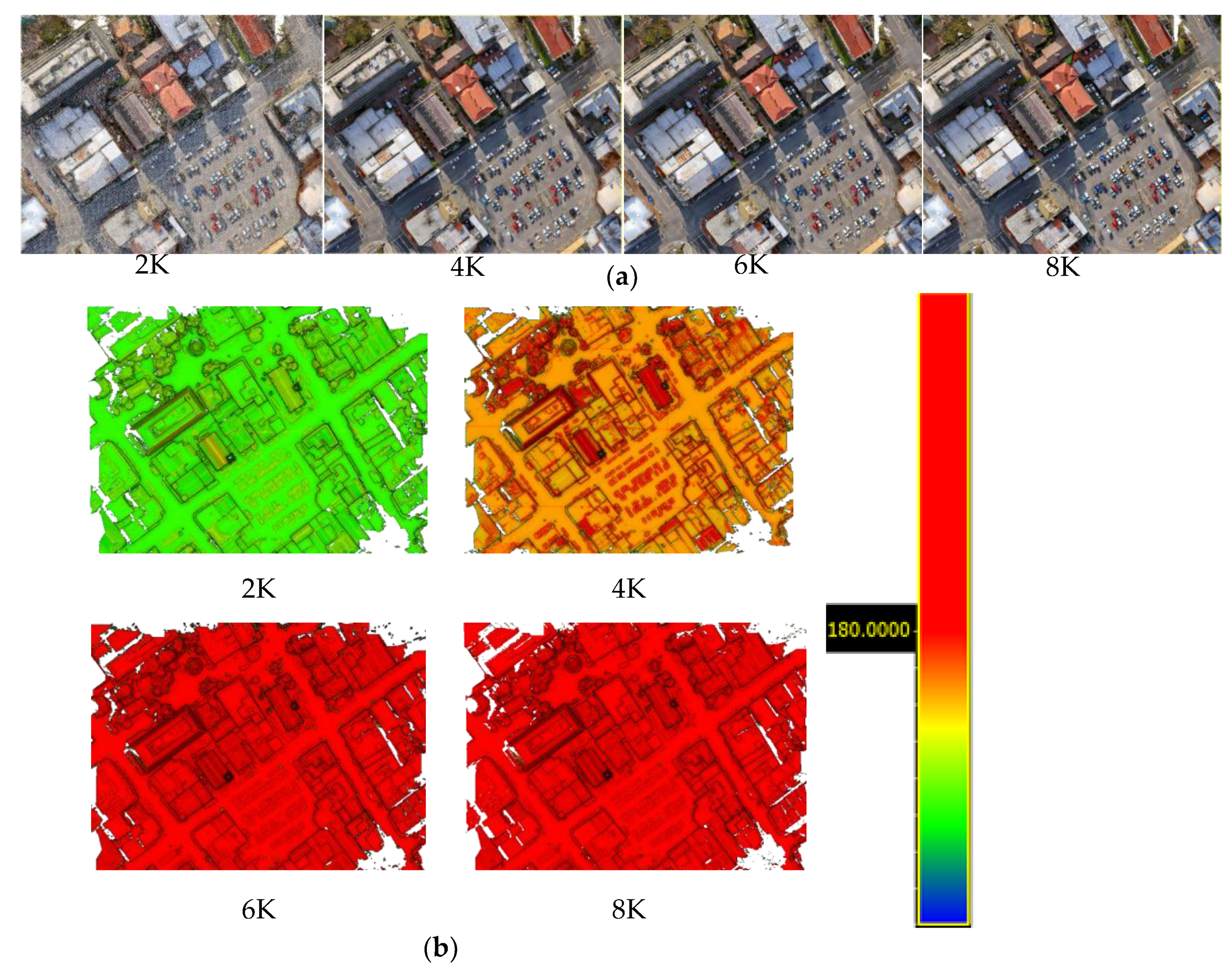
To clarify by how much the point cloud densities differ among the four video resolutions, color-coded figures are created showing the point densities at each resolution (Figure 8) where point densities above 180 pts/m² are colored in red. We considered density average > 180 pts/m² is sufficient for urban 3D city modeling applications from drones where fine structural details can be modeled [30].

Furthermore, orthomosaics are created for the area using the four video resolutions to test the pictorial quality of these orthoimages and to compare visually the differences between them. Figure 9 shows differences in orthomosaic resolutions and clarity. A summary is shown in

Table 1. Orthomosaic resolution and pixel size of the first experiment.

	2K	4K	6K	8K
Orthomosaic resolution	4367 × 3722	9348 × 7370	16,805 × 12,805	21,327 × 17,659
Orthomosaic pixel size (GSD)	7.3 cm	3.7 cm	2.5 cm	1.8 cm

using the four video resolutions and the pixel size of every created orthomosaic.

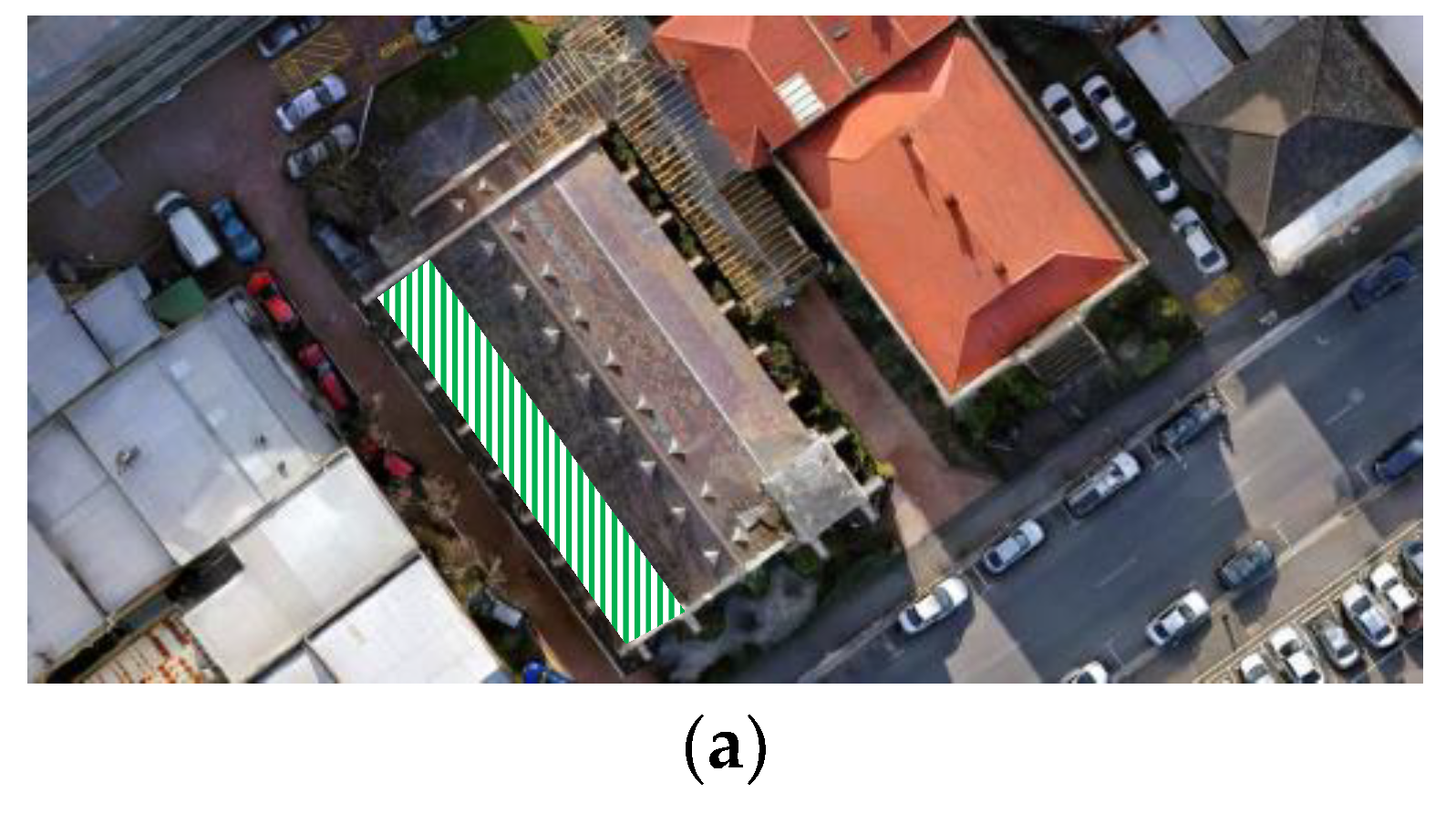
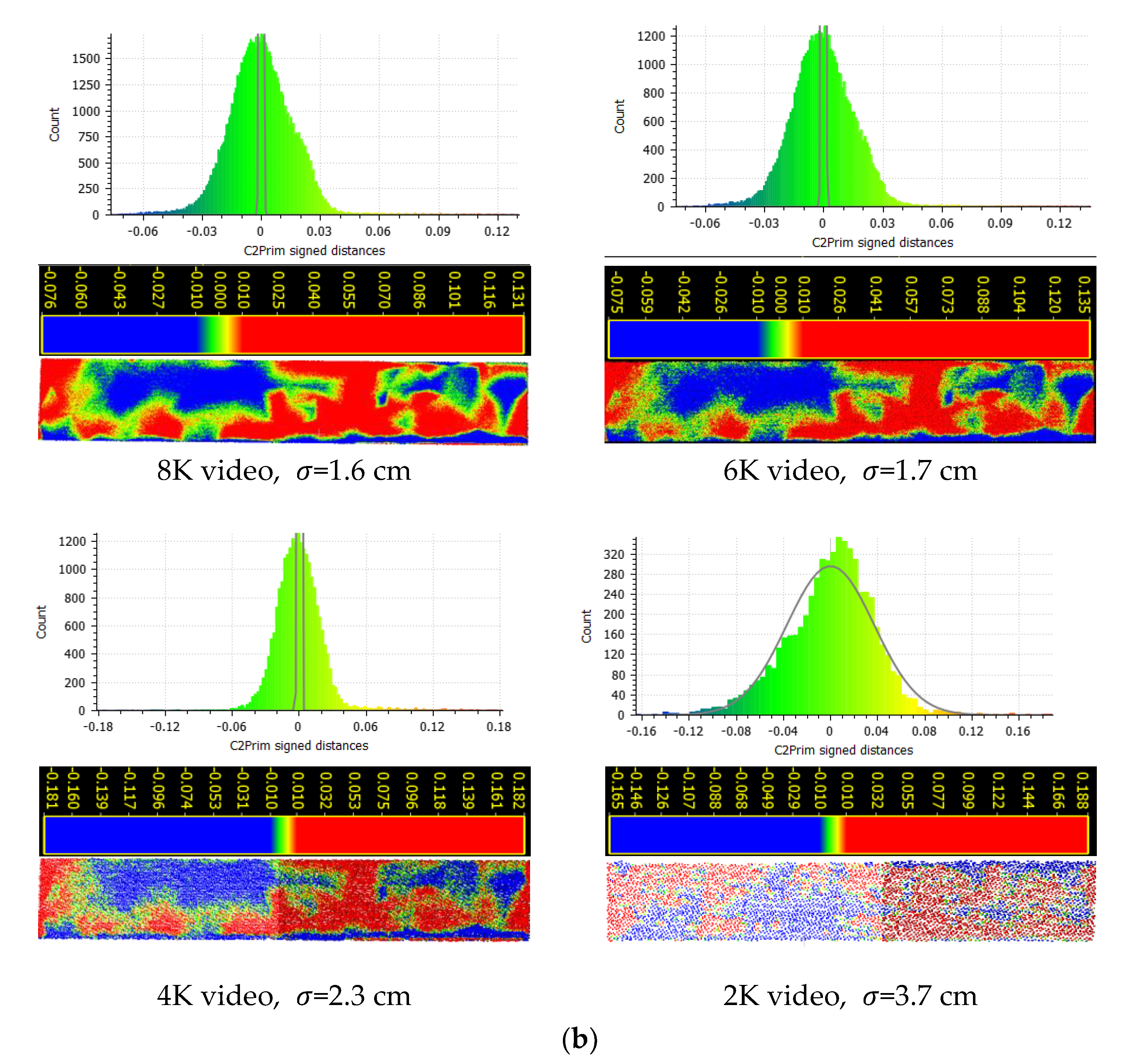
Moreover, to evaluate the achieved relative accuracy between the four video resolutions, a planar roof slab of a church building is selected as shown in Figure 10a. Every created point cloud is cropped and then the best plane fitting is applied and residuals are computed. Then, the standard deviation $\sigma$ to the best-fit plane is computed assuming a Gaussian distribution as shown in Figure 10b where the distance between the points and the best fit planes are also visualized.

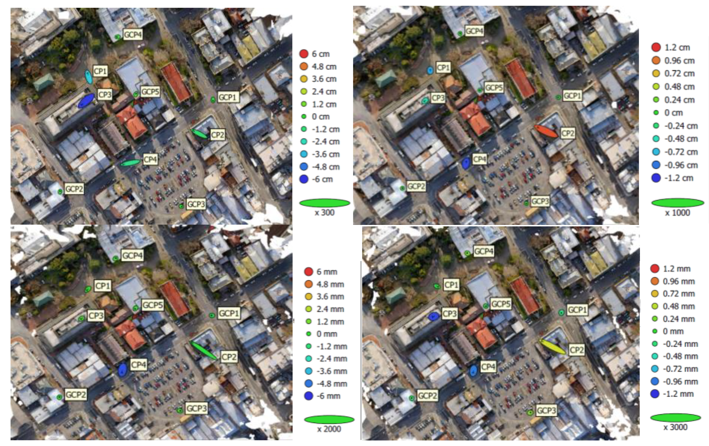
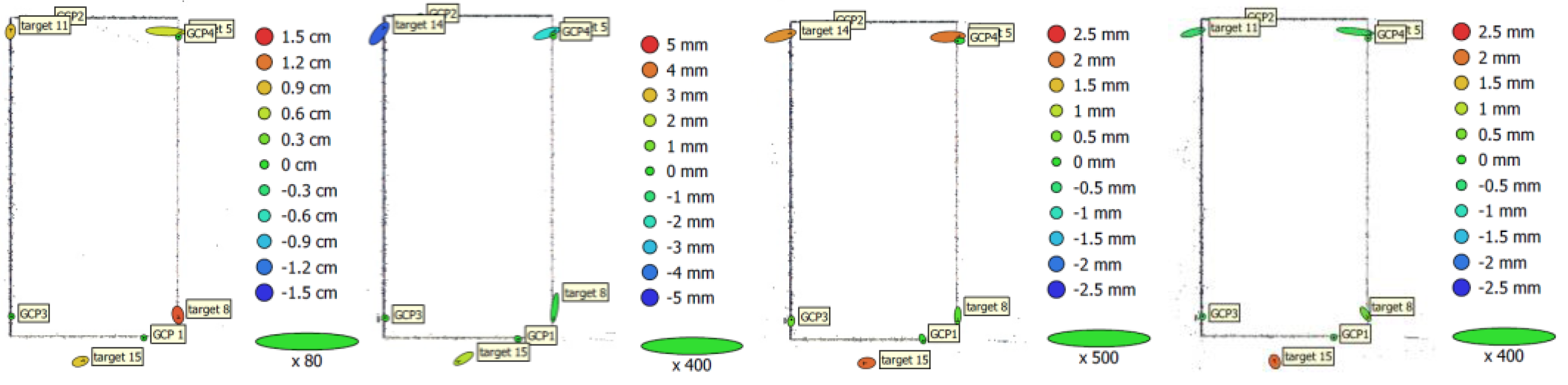
For external accuracy assessment, we used nine reference points represented by one squared-meter coded target distributed all over the area where five are used as GCPs and four as checkpoints.

Table 2. Estimated RMSE at the four checkpoints distributed over the area at the four drone video resolutions.

		Using 2K Video	Using 4K Video	Using 6K Video	Using 8K Video
	RMSE X [mm]	35.8	8.1	6.0	3.7
	RMSE Y [mm]	21.9	4.3	4.7	2.1
	RMSE Z [mm]	34.7	9.0	2.7	0.8
	RMSE Total [mm]	54.4	12.9	8.2	4.3

and Figure 11 illustrate the RMSE achieved in the checkpoints. Noticeably, the coded targets are not detected at the 2K drone video, only two at the 4K video, most of the targets at the 6K video, and the full target set at the 8K video. Reasonably, this is highly related to the video resolution and GSD values.

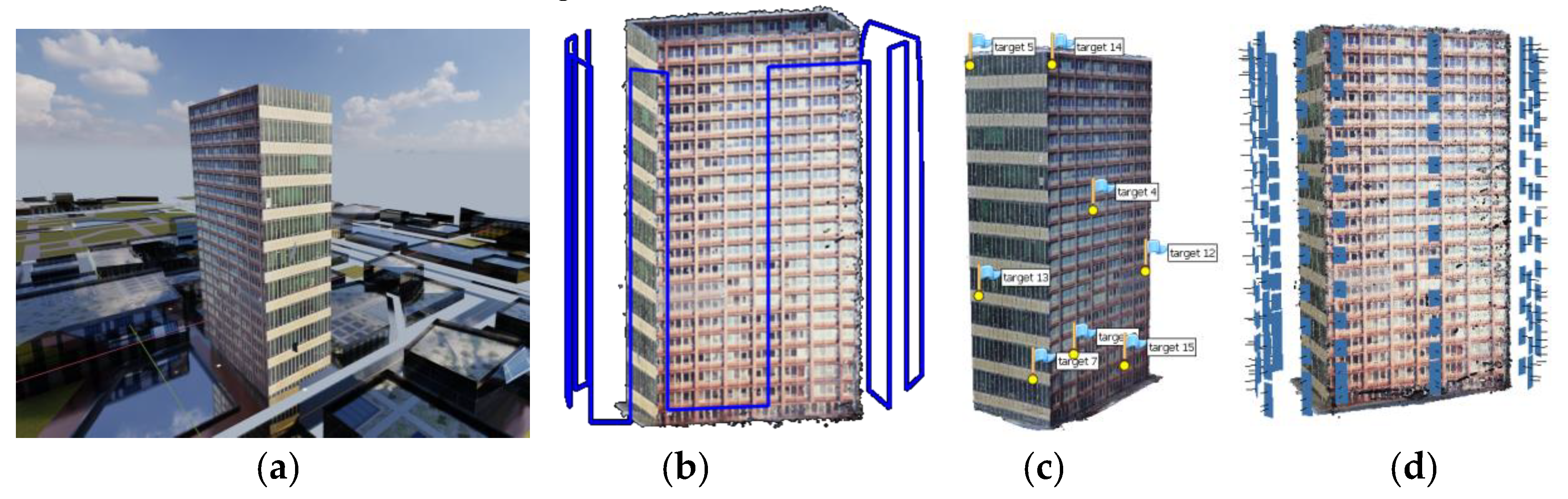
2nd experiment: tall city building.

The second test is applied for a city building of 70 m height above the ground [27] as shown in Figure 12a. Similar to the first experiment, four drone videos are captured around the building of 2K, 4K, 6K, and 8K, respectively, by simulating a flight of DJI Phantom 4 Pro using the following flight parameters:

Focal length = 8.8 mm

Pixel size = 2.37 µm

Sensor dimensions =13.2×8.8 mm

Imaging distance = 30 m

Flight speed = 5 m/s

Forward overlap = 80% and side overlap = 60%

Accordingly, 277 video frames are used along the flight strips around the building facades as shown in Figure 12b. A video illustrating the flight mission around the building is shared in [31] as a Supplementary Materials. Several GCP targets are placed on the building facades and on the ground shown in Figure 12c to have a correct scaling and orientation (Figure 12d).

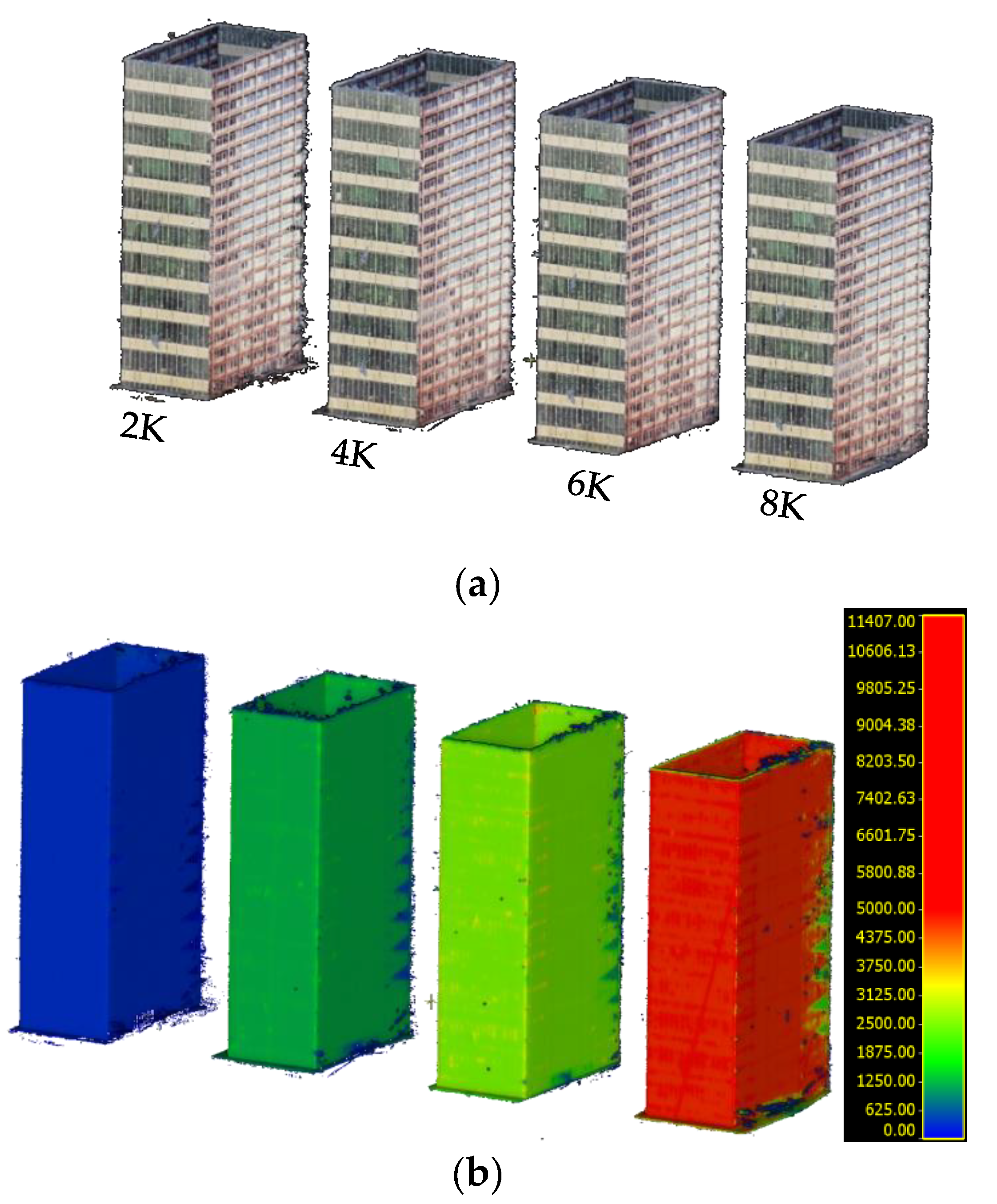
The rendered drone images are processed in the Metashape tool for each captured video resolution by applying the image orientation followed by the dense reconstruction to create a dense point cloud of the building (Figure 13a). It is worth mentioning that the acquired point clouds of the building are created using only ¼ full resolution of the frames (medium setup in Metashape tool) to reduce the processing time.

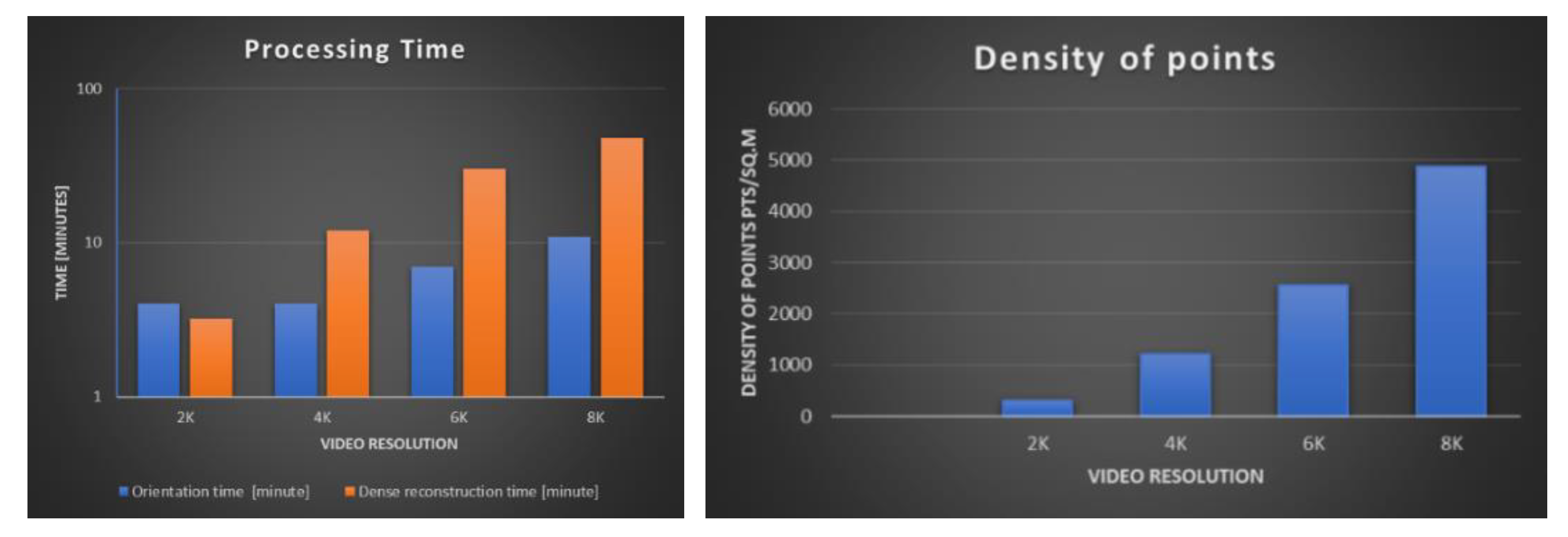
In Figure 14, two histograms are shown to clarify the relationship between the time consumed in creating point clouds and point densities with respect to the recorded video resolution.

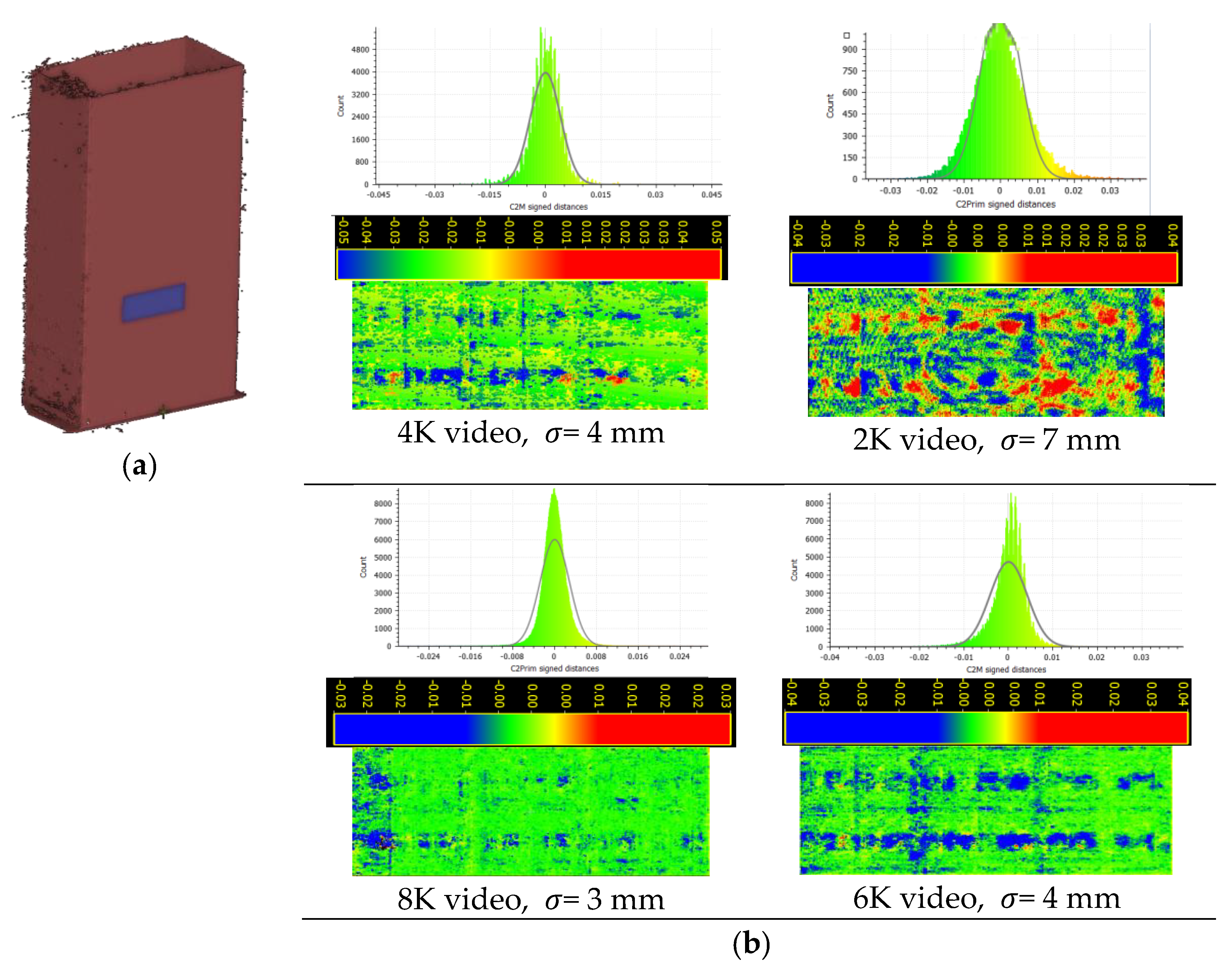
As in the first test, an evaluation of the achieved relative accuracy between the four video resolutions is applied. A planar façade patch is selected as shown in Figure 15. Every created point cloud is cropped and then the best plane fitting is applied and residuals are computed. Then, the standard deviation $\sigma$ to the best-fit plane is computed assuming a Gaussian distribution as shown in Figure 15 where the distances (residuals) between the points and the best fit planes are also visualized where the red and blue colors indicate > ±1 cm errors.

For external accuracy assessment, we used the same GCPs placed around the building facades and saved others as checkpoints.

Table 3. RMSE estimated at the checkpoints distributed over the building facades at the four drone video resolutions.

		Using 2K Video	Using 4K Video	Using 6K Video	Using 8K Video
	RMSE X [mm]	24.8	3.6	4.8	5.6
	RMSE Y [mm]	6.8	4.3	1.6	1.6
	RMSE Z [mm]	9.7	2.7	1.7	1.1
	RMSE Total [mm]	27.5	6.3	4.7	5.9

and Figure 16 illustrate the RMSE achieved in the checkpoints.

For one facade of the building, orthomosaics are created using the four video resolutions and the size and pixel size of every created orthomosaic is summarized in

Table 4. Orthomosaic resolution and pixel size of the second experiment.

	2K	4K	6K	8K
Orthomosaic resolution	3588 × 6320	7288 × 12,334	12,638 × 23,366	13,525 × 23,988
Orthomosaic pixel size	12 mm	6 mm	4.4 mm	3.2 mm

.

4. Discussion

Based on the results of the two experiments shown in the previous Section 3 and as summarized in

Table 5. Summary of results.

	Video Resolution	Number of Points (million)	Density pts/m2	Orientation Time (minute)	Dense Reconstruction Time (minute)	Average GSD(cm)
First experiment	2K	1.4	42 ± 8	≅1.0	≅3	7.3
	4K	22.0	168 ± 33	≅1.0	≅13	4.5
	6K	49.0	378 ± 76	≅1.5	≅28	2.5
	8K	88.0	674 ± 139	≅2.5	≅71	1.8
Second experiment	2K	3.8	318 ± 46	≅4	≅3.2	1.24
	4K	14.5	1216 ± 142	≅4	≅12	0.64
	6K	30.0	2555 ± 318	≅7	≅30	0.44
	8K	57.8	4866 ± 670	≅11	≅48	0.32

, several observations are made and clear comparisons between the different video frame derived models are found as follows. Logically, the point density increase was related to the video frame resolution increase which is also connected to the achieved GSD values as shown in Figure 17. This is also observed in the produced orthomosaics (Table 2 and Table 4) where the pixel sizes much decreased and then more details are expected to be seen (large-scale) on the orthomosaic.

What was found to be interesting is the improved internal relative accuracy whenever the video frame resolution increased. The improvement is recorded with up to 50% when using 8K videos compared with the HD videos. This means that the derived point clouds at the UHD videos are less noisy compared with the point clouds derived from HD videos.

The external accuracy in both experiments indicated improvements whenever the video frame resolution increased. More than ten times improvement was found in the first experiment and three times in the second test when using 8K videos compared with the HD videos.

It is worth mentioning that measuring the GCP targets either automatically or manually on the HD images is challenging due to the low resolution or the larger GSD which might cause the degraded external accuracy. A significant improvement in point densities is recorded in both experiments with around a 90% increase when using 8K videos compared with the HD videos (Table 5). It should be noted that the acquired point clouds were created using half and ¼ of the full image resolution in the two experiments, respectively, to reduce the processing time.

UHD video-based 3D modeling requires larger computer memory and entails time consumption as shown in Figure 7 and Figure 14. This is expected to be reduced with the continuous developments in the capabilities of the computers and the increase in offered cloud services and solutions. 3D models created using HD videos are of low quality and cannot be used for projects that require highly detailed and highly accurate results.

Table 5 shows the summary of results achieved in both experiments for better comparison.

The achieved point densities and accuracies are shown when using UHD drone videos to enable several applications. According to [32], applications include but are not limited to the following: engineering surveying, road pavement monitoring, cultural heritage documentation, digital terrain modeling, as-built surveying, and quality control. Furthermore, it is also suitable for building information models (BIM) and CAD, power line clearance, GIS applications, slope stability and landslides, virtual tours, etc.

5. Conclusions

In this paper, the impact of using UHD video cameras (6K and 8K) onboard drones was investigated on the 3D reconstructed city models. Furthermore, these UHD video-based models are compared with the same 3D models produced from the currently used HD and 4K cameras. The results were investigated in two simulated flights applied in urban environments following grid flight paths around or above city buildings as shown in Figure 6 and Figure 12. In both experiments, it was shown that increasing the video resolution not only improved the density but also the internal and external accuracies of the created 3D models. As shown in Table 5, the point density and the reconstruction accuracy were improved up to 90% when using 8K videos compared with the HD videos taken from the same drone. Noticeably, the GSD was improved around four times when the 8K image resolution was used compared with the HD resolution while maintaining the same flying height. This improvement will guarantee high details of the reconstructed 3D models and hence opens a wide range of applications for using drones equipped with 8K video cameras for roadway condition assessment, powerline clearance, cultural heritage restoration and documentation, as-built surveying, etc.

However, it is still a challenge when using the UHD videos where the memory required, the processing power needed for the computations, and the time consumption could be increased by more than 20 times on average. Therefore it is recommended to continue the research to find a solution for big data handling and finding on-the-fly or cloud-based solutions to speed up the data handling and the geoinformation data extraction.

Worth mentioning, the simulated video frames were blur-free since the videos are rendered in typical flight stabilization. This is to be considered for future simulation experiments to mimic reality