
Spatially Varying Effects of Street Greenery on Walking Time of Older Adults


1
Department of Urban and Rural Planning, School of Architecture and Design, Southwest Jiaotong University, Chengdu 611756, China
2
Department of Urban Planning and Design, Faculty of Architecture, The University of Hong Kong, Hong Kong 999077, China
3
Urban Mobility Institute, Tongji University, Shanghai 200092, China
4
Department of Architecture and Civil Engineering, City University of Hong Kong, Hong Kong 999077, China
5
School of Transportation and Logistics, Southwest Jiaotong University, Chengdu 611756, China
*
Author to whom correspondence should be addressed.
ISPRS Int. J. Geo-Inf. 2021, 10(9), 596; https://doi.org/10.3390/ijgi10090596
Submission received: 2 August 2021
/
Revised: 9 September 2021
/
Accepted: 9 September 2021
/
Published: 10 September 2021
(This article belongs to the Special Issue Advancements in Geospatial Planning and Assessment of Green Infrastructure in Cities of the Future)
Abstract
:Population aging has become a notable and enduring demographic phenomenon worldwide. Older adults’ walking behavior is determined by many factors, such as socioeconomic attributes and the built environment. Although a handful of recent studies have examined the influence of street greenery (a built environment variable readily estimated by big data) on older adults’ walking behavior, they have not focused on the spatial heterogeneity in the influence. To this end, this study extracts the socioeconomic and walking behavior data from the Travel Characteristic Survey 2011 of Hong Kong and estimates street greenery (the green view index) based on Google Street View imagery. It then develops global models (linear regression and Box–Cox transformed models) and local models (geographically weighted regression models) to scrutinize the average (global) and location-specific (local) relationships, respectively, between street greenery and older adults’ walking time. Notably, green view indices in three neighborhoods with different sizes are estimated for robustness checks. The results show that (1) street greenery has consistent and significant effects on walking time; (2) the influence of street greenery varies across space—specifically, it is greater in the suburban area; and (3) the performance of different green view indices is highly consistent.
1. Introduction
Population aging is a notable demographic phenomenon worldwide. It has been widely observed in a myriad of developed and developing countries/regions. Low fertility (or childbearing) and prolonged lifespan contribute to this trend, and the former is the major contributor [1]. Hong Kong, an international city with over 7.5 million residents [2], has evidently grappled with the conundrum of aging for years. In 2019, Hong Kong held 1.32 million older adults and had the second-highest percentage (17%) of older adults (defined as those aged 65 years or above) in Asia (the continent expeditiously shifting from being predominantly young to being primarily old), which was exceeded only by Japan [3]. The number and proportion of older adults are predicted to increase to 2.69 million and 34%, respectively, in 2049 [3]. Therefore, catering for the future vigorous increase in the number and proportion of older adults in Hong Kong is indispensable.
Travel is an indispensable component of life for everyone (irrespective of age) [4]. For older adults, mobility (often defined as the ability to travel) is closely associated with independence, quality of life, subjective wellbeing, and social integration [5]. It is also one of the ingredients of active aging [6]. Therefore, improving the mobility of older adults is exceedingly important for bolstering social development and should be prioritized in future policy measures, especially in the population aging period. Evidently, understanding the travel behavior of older adults is the first and foremost step toward the abovementioned goal.
Walking is a popular travel mode for older adults [7]. It is effortlessly fused into a daily routine and easily promoted or hindered by numerous interventions [8]. Moreover, walking has a wide variety of health, economic, environmental, and social benefits, and it helps promote healthy aging and active aging, which are essential for older adults. As the most prevailing aerobic exercise, walking requires the physical activity of human beings and helps beat the notorious sedentary and inactive lifestyle. Therefore, it increases individuals’ physical and mental health and lowers the risk of numerous non-communicable diseases (e.g., type 2 diabetes) [9].
The built environment is a known and extensively studied concept in fields such as geography, environmental science, transportation, public health, and urban planning [10]. Recently, with the advancement of science and technology (e.g., compute vision as well as deep learning algorithms) [11,12,13], street greenery, a built environment factor that cannot be easily assessed by traditional approaches, can now be accurately calculated based on street view imagery (e.g., Google, Baidu, and Tencent) data, which effectively describe real-world scenery [14,15]. Therefore, it has recently attracted scholarly attention. Many travel studies that used street view imagery data to measure neighborhood built environment have sprung up in the past couple of years. However, only a handful of previous studies have examined the link between street greenery and the walking behavior of older adults.
The spatial heterogeneity (or nonstationarity) in the connection between street greenery and the walking behavior of older adults is an issue of high relevance for research and practice. In other words, an enriched understanding of such links is of great importance as it serves as a valuable reference for evidence-based interventions to promote walking and increase physical activities for older adults. Inspired by recent empirical studies focusing on the spatially heterogeneous relationship between travel behavior and numerous built environment factors [16,17], we reasonably assume that spatial heterogeneity exists in the association between older adults’ walking behavior and street greenery. However, to our best knowledge, no previous studies have been devoted to this issue. To address the above issues and fill the gap left by previous research, we used Hong Kong as the study area and extracted the socioeconomic and walking behavior data of older adults from the Travel Characteristic Survey (TCS) 2011. More importantly, we used Google Street View (GSV) imagery and the fully convolutional neural network (FCN-8s), a machine learning technique, to evaluate neighborhood-level street greenery. A set of geographically weighted regression (GWR) models was developed to characterize the spatially heterogeneous effect of street greenery (with various neighborhood definitions) on the walking time (walking duration) of older adults. Inspired by previous studies, three distance thresholds, namely 400 m, 800 m, and 1600 m, were selected. Finally, we discussed the empirical findings and proposed implications for research and practice. Notably, to our best knowledge, this study is the pioneer in scrutinizing the spatially heterogeneous relationship between street greenery and the walking behavior of older adults.
The contributions of this study include the following: (1) examining the relationship between street greenery and the walking behavior of older adults; (2) advancing the understanding of the spatial heterogeneity in the relationship; and (3) comparing the performance of several street greenery measures in neighborhoods with different sizes (400 m, 800 m, and 1600 m).
The remainder of this paper is as follows. Section 2 offers a review of the literature focusing on the correlates of older adults’ walking behavior. Section 3 and Section 4 introduce the data and modeling approaches, respectively. Section 5 presents the global and local modeling results. Section 6 reveals the implications for research and practice and research limitations. Finally, Section 7 summarizes the findings and winds up the paper.
2. Literature Review
Numerous studies have been conducted by researchers from transport, public health, and urban planning fields to identify the correlates (or determinants) of older adults’ walking behavior (more broadly, physical activity). The correlates can be mainly categorized into three groups, namely socioeconomic characteristics (e.g., gender and age), neighborhood built environment factors (e.g., population density and proximity to opportunities), and attitudinal attributes (e.g., preference for walking) [18,19]. A wide variety of modeling approaches, including linear regression models [20], discrete choice models (e.g., binary logistic regression models and multinomial logit models) [21], Poisson or negative binomial regression models [22], zero-inflated ordered probit models [7], Cox proportional hazards models [7], and structural equation models [23], have been used. Recently, machine learning techniques, such as random forest, have been introduced into this research field [24]. Moreover, some studies have not focused on overall walking but divided walking into two categories, namely transportation (utilitarian) walking and recreational (leisure) walking according to travel purposes [25]. Furthermore, many studies, especially those from the public health field, have concentrated on physical activities (roughly equivalent to walking + cycling) instead of walking. Interested readers can refer to two systematic literature reviews on the physical environment and older adults’ physical activity (mostly walking) [18,19] and Yang et al.’s summary [26] for more information.
Among the socioeconomic characteristics examined, age and gender elicited the greatest scholarly attention. Findings on the links between age and walking behavior are relatively consistent. Most, though not all, studies have concluded that for older adults, age negatively affects walking time and frequency [27,28]. A strong explanation is that mobility quintessentially reduces with age because of physical decline (physical frailty). However, the role of gender in shaping older adults’ walking behavior is not so clear-cut. Mixed, even conflicting, findings are obtained. For example, Yang et al. [20] suggested that men have higher walking frequency and time, whereas Zang et al. [27] concluded that gender plays an insignificant role in determining walking time. Notably, the above two studies with distinct findings have been conducted in the same city, namely Hong Kong. Furthermore, the contributing role of other socioeconomic characteristics, such as income, education attainment, personal/family car availability, job status, transit pass availability, mobile phone availability, dog ownership, marriage status, and residence condition, has been empirically assessed [18,19].
The built environment, which is usually measured in the “3Ds”, “5Ds”, or “7Ds” framework (including a variety of D variables, namely density, diversity, design, destination accessibility, distance to transit, demand management, and demographics), has been extensively shown to significantly affect the walking behavior of older adults. A host of built environment factors (e.g., population density and proximity to parks and open spaces) have been determined to significantly associate with older adults’ walking behavior. Many studies have concluded that when the built environment is well planned/designed and has good attributes, walking can be popular among residents. Moreover, they reached some relatively consistent conclusions. For example, a sufficient amount of evidence of positive connections between density/diversity/walkability and the walking propensity/time/frequency of older adults was found [18]. However, a few contradictory findings are still obtained. For example, walking/cycling facilities have been shown to have positive, insignificant, or adverse effects on the physical activity of older adults [19].
Nevertheless, the significant role of the built environment is also challenged and questioned in a modicum of research. For example, Yang et al. [20] argued that five out of six built environment factors, including population density, land use mix, and proximity to retail shops, are too weak to influence the walking time of older adults in Hong Kong; the only significant built environment factor is proximity to recreational facilities.
As the built environment attribute of our primary interest, street greenery has been examined in elderly walking behavior studies. Zang et al. [27] investigated the walking time of 180 older adults in six regions in Hong Kong. They identified its positive relationship with street greenery, which is measured by the manual extraction of green pixels in Baidu street view imagery. Zang et al. [28] observed that street greenery, which is assessed by a machine learning technique, has significant effects on the walking propensity and time of older adults in private housing but has no discernable impact on that of older people in public housing. Similarly, Yang et al. [20] scrutinized the effect of street greenery on older adults’ walking propensity and time and determined a significantly positive effect. In a departure from the above two studies employing regression methodologies, Yang et al. [26] assumed the nonlinearity in the relationship between street greenery and the walking propensity of older adults in Hong Kong. They thus adopted a machine learning approach, namely random forest, to decipher such a complex relationship and demonstrated that the effect of street greenery is not unconditional: the greenery has a positive effect only with a particular range.
In comparison with the above two correlate categories (i.e., socioeconomic characteristics and neighborhood built environment factors), attitudinal attributes have been examined considerably less frequently. Handy et al. [29] carried out a quasi-longitudinal analysis in Northern California and examined the contributory role of attitudinal attributes on walking behavior. They concluded that attitudinal attributes, such as pro-bike/walk attitude and pro-transit attitude, play a significant role in determining the residents’ walking behavior. Larrañaga et al. [30] observed that the pro-walk attitude significantly affects residents’ transport and recreation walking behavior in a Brazilian city. Cheng et al. [7] observed that preferences for walking and cycling have a marginal effect on active travel frequency and time in Nanjing, China. Likewise, such preference variables are incorporated into the travel behavior modeling framework of [31].
All in all, numerous theoretical and empirical studies have been conducted on the identification of the correlates of older adults’ walking behavior. However, studies focusing on street greenery are limited. More importantly, no studies have examined spatially heterogeneous links between street greenery and older adults’ walking behavior.
3. Data
3.1. Travel Data
About every ten years, the Transport Department of the Hong Kong government conducts a large-scale voluntary survey (i.e., TCS) to collect timely data on residents’ travel behavior to aid transportation planning and policymaking. Previous surveys were conducted in 1981, 1992, 2002, and 2011. The most recent one was performed in 2011.
The TCS 2011 survey consists of three sections, namely Household Interview Survey on residents’ trip information, Stated Preference Survey on factors influencing choices of travel means, and Hotel/Guesthouse Tourists Survey on trip information of hotel/guesthouse-staying tourists. The Stated Preference Survey was conducted on selected Household Interview Survey sampled household members who matched the market segment criteria relevant to the respective Stated Preference survey topics. That is, the respondents of the Stated Preference Survey are a subset of those of the Household Interview Survey. Moreover, some personal characteristics of the respondents, such as name and accurate residence address, are not recorded.
The cornerstone of the TCS 2011 survey is the Household Interview Survey. It is a weekday survey in which 101,385 residents in 35,401 families participated. The sampling rate is about 1.5%. The Household Interview Survey covers three levels: (1) family-level data (e.g., monthly income, housing address, and housing category); (2) family member-level data (e.g., gender, job, job industry, and age); (3) trip-level data (24-hour trip records for each family member, including but not limited to trip starting and ending points and time, transport modes, interchanges, and trip legs). As travel-related socioeconomic characteristics and trip characteristics are included in the TCS 2011 data, statistical models can be calibrated to explore the underlying mobility behavior mechanism of older adults.
We extracted the walking behavior data of older adults (people aged 65 years or above) from the Stated Preference Survey (Attachment Survey 2, “Travel Propensity, Walking and Use of Travellator”), which accurately characterizes the walking behavior of the respondents. This survey only documents trips in which no mechanized transport was involved during the reference 24-hour period. The origin, destination, start time, and end time of the trips are recorded. However, other walking trips, such as those linking transit (first-mile walking and last-mile walking), are not recorded.
Based on the TCS 2011 data, we geo-coded respondents’ residential locations in the mapping and analytics software ArcGIS (Version 10.6) for neighborhood built environment evaluation.
3.2. Street Greenery Data
Street view imagery accurately records 360-degree high-resolution views of physical environments in a way that resembles human vision. Its advantages over mainstream data sources include widened coverage, limited data bias, time-effectiveness, and cost-efficiency [14]. The earliest online street view service is GSV, which started in 2007 and has since covered cities from about 90 countries [32]. GSV mainly gathers data through the Global Positioning System tools installed on sensing cars.
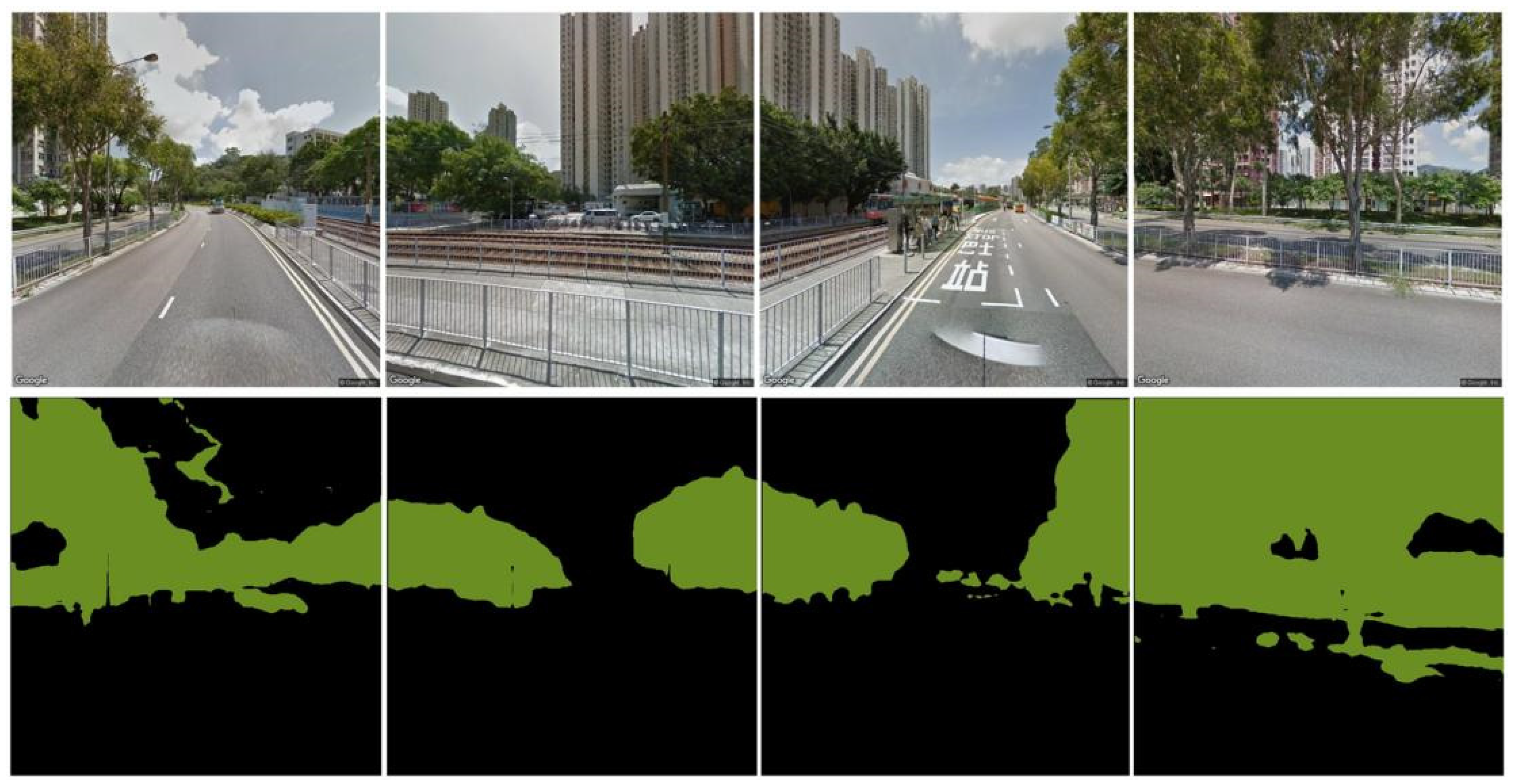
GSV can be used to estimate the green view index (or eye-level street greenery index) to simulate people’s perception of street greenery. First, GSV geocodes the coordinates (latitude and longitude) of residential locations into the ArcGIS platform. Second, the platform automatically recognizes street segments near geocoded locations. Third, GSV-related positions are finalized in intervals of 50 m. Fourth, corresponding GSV images are loaded from Google Maps: four mutually exclusive and collectively exhaustive images represent a 360-degree panoramic of each GSV position. Fifth, the fully convolutional neural network (FCN-8s), a machine learning technique, is used to identify greenery pixels from the images (see Figure 1) [33]. This technique, which is based on semantic segmentation, can exclude green facilities and buildings, guaranteeing its (relative) accuracy. For each GSV-generating position, the calculation formula for the green view index is:
The fully convolutional neural network has been adopted by numerous street view imagery-based studies, and its applicability has extensively been validated. Moreover, to further confirm the acceptability of the algorithm’s performance, results from our approach are compared with those from manual extraction in Adobe Photoshop software. The greenery pixels of thirty randomly chosen GSV images are extracted by student helpers. The green view indices calculated by the two methods have been analyzed by a Pearson’s correlation test. The analysis outcome reveals a high correlation (r > 0.90), indicating the excellent performance of our algorithm.
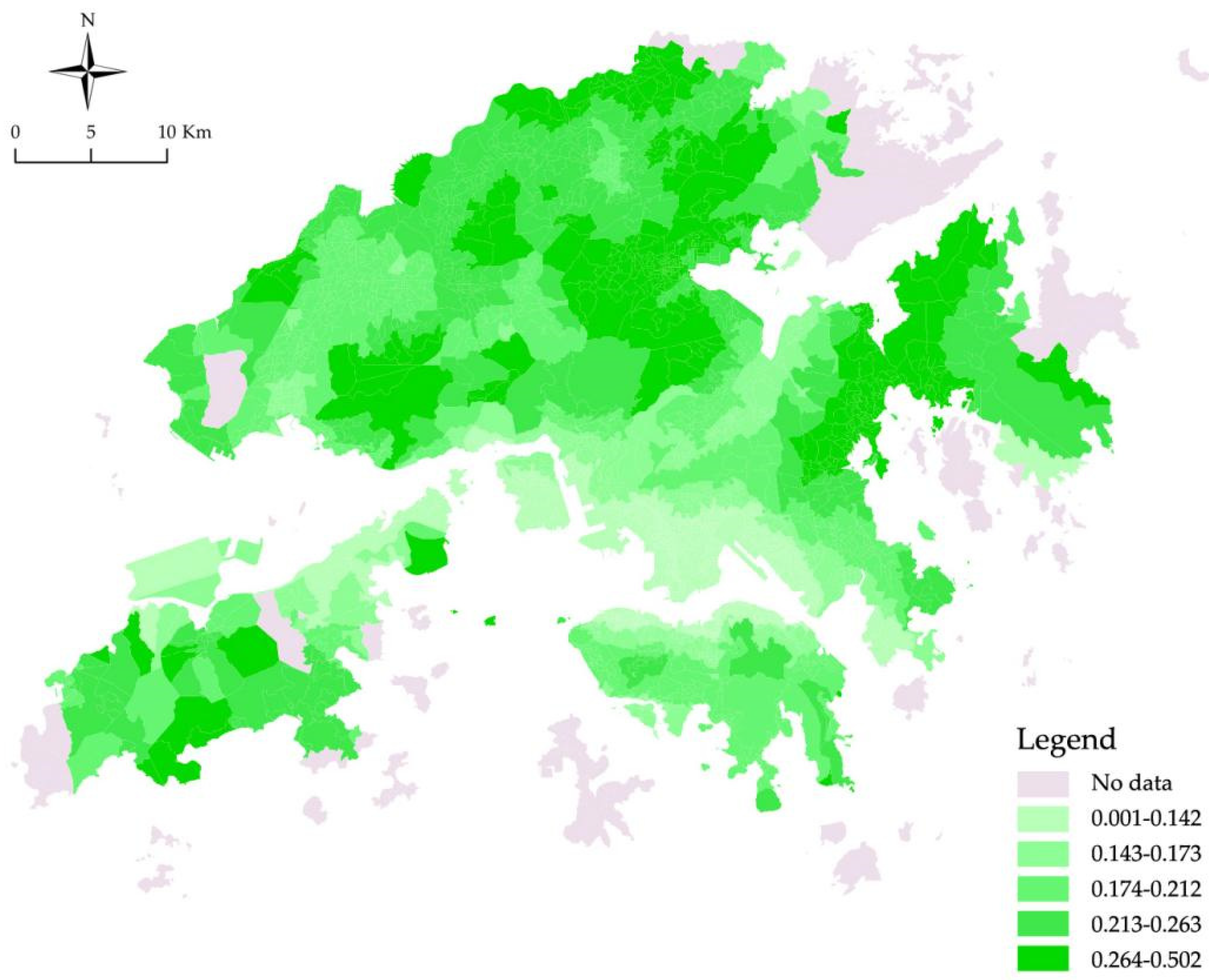
Figure 2 reveals the geographical distribution of the green view index. The index is normally lower in the urban area (Hong Kong Island and Kowloon) but higher in the suburban area (the New Territories).
3.3. Built Environment Data
The built environment is a multi-facet concept and can be measured from a series of dimensions. A widely accepted built environment assessment approach is the “3Ds” model [34], or its enhanced version, the “5Ds” or “7Ds” model [35]. Inspired by the “5Ds” model, this study evaluates many built environment variables, including density, diversity, and destination accessibility. A built environment analysis framework is developed in ArcGIS (Version 10.6) based on data from OpenStreetMaps (https://www.openstreetmap.org, accessed on 8 September 2021).
4. Methods
4.1. Global Models
The response variable, the walking time of older adults, is a continuous variable. Therefore, a linear regression model is developed to examine the association between the response and independent variables. The linear regression model can be expressed as
where is the response variable at observation i (walking time in this study); k is the index of the independent variables; is independent variable k at observation i; and are the intercept and the coefficient of independent variable k, respectively; and is an error term at observation i, which captures the collective effects of uncaptured factors on the response variable ().
The linear regression model predefines a linear functional form and assumes that the connection between the response and independent variables is linear. As one of its alternatives, the Box–Cox transformed model, a typical nonlinear regression method, relaxes the linearity assumption and makes error terms closely follow the normal distribution. It is used to search for the best model specification by maximizing the model log-likelihood and has been extensively used in empirical studies with continuous response variables [36]. Generally, the Box–Cox transformed model can be expressed as
where for ≠ 0, for ≠ 0, while for , for ; and other parameters are defined as before. The response variable is Box–Cox transformed by parameter , while independent variables are Box–Cox transformed by parameter . Notably, variables that are not constantly positive are untransformed.
4.2. Geographically Weighted Regression (GWR) Models
In a departure from traditional regression models that use a sole equation to characterize the link between the response and independent variables, the GWR model develops a set of equations to capture the potential presence of spatial heterogeneity in the relationship. Each regression point has its own equation, which is estimated using this point and its neighborhood points (a subset of sample points in most cases). In other words, the GWR model expands the traditional regression framework by relaxing the space-invariant relationship assumption, thereby allowing point-varying parameters to be estimated [37]. It is employed in numerous empirical studies [38,39,40], and its formula can be expressed as
where represents the projected or spherical coordinate of observation (point) i; and are the intercept and the coefficient of independent variable k, respectively, in the local equation of observation i; and other parameters are defined as before.
Four kinds of kernel functions are commonly used to weight “neighbors” (nearby points) for local equation estimation, which is based on the weighted least square method. They include:
Fixed Gaussian kernel function:
Adaptive Gaussian kernel function:
Fixed bi-square kernel function:
Adaptive bi-square kernel function:,
where is the weight of nearby point j for point i’s equation estimation; is the straight-line distance between points i and j; is the fixed bandwidth; and is the adaptive bandwidth, which hinges on the kth closest-neighbor distance for point i’s equation. All kernel functions are monotonically nonincreasing to ensure that they agree with Tobler’s first law of geography [41]. Among the four functions, fixed Gaussian and adaptive bi-square kernel functions are the most extensively used in the existing literature [42]. Furthermore, the selection of the optimal kernel function and the bandwidth often relies on the corrected Akaike information criterion (AICc) [43].
4.3. Variables
Following the existing literature and considering data availability, a total of nine variables, including four socioeconomic and five built environment variables, are selected as control variables (Table 1). Moreover, a set of street greenery variables with varying neighborhood definitions (distance thresholds) is created to verify the robustness of our primary findings. Other popular greenness variables that often have high correlations with street greenery, such as the Normalized Difference Vegetation Index (NDVI) and the number of parks in the neighborhood, have not been incorporated, as Yang et al. [44] pointed out that they play a limited role in shaping elderly mobility. In addition, the metro, which is the backbone of Hong Kong’s advanced transit system, is considered in the selection of distance-to-transit variables, following the existing literature [20,28,45]. Moreover, inspired by [20], recreational facilities, a popular destination for older adults, are considered.
5. Results
5.1. Global Results
Three linear regression models are developed to estimate the global association between street greenery (evaluated by three variables) and the walking time of older adults. Table 2 shows the results. Age affects walking time negatively. A compelling explanation is that mobility typically decreases with advancing age, due largely to physical decline and loss of functional abilities. In other words, age is a good predictor of walking time for older adults. The very old, who likely live with diseases and frailties, always perform few outdoor walking activities. In addition, family size is adversely related to walking time. A possible explanation is family responsibility sharing [46]. In China, older adults commonly receive much material and spiritual support. If living with others (e.g., relatives and friends), they may not need to walk out to complete family tasks (e.g., going to supermarkets and vegetable markets) in most cases. Instead, they can easily entrust the tasks to other family members. Moreover, access to the metro is too weak to shape walking time for older adults. A possible explanation is that as two travel modes, walking and the metro have both complementary and substitutionary relationships. Therefore, access to the metro may either increase or decrease walking frequency/time [20]. Furthermore, access to recreational facilities positively affects walking time. This finding is consistent with [20,47,48].
The interpretation of street greenery variables is of predominant interest here. We find that their performance is highly consistent across the three models. That is, the variables are significant at the 1% level. This observation resonates with [20,26,27]. Ample evidence documents a positive association between street greenery and the walking time of general residents, public housing residents, or older adults. In addition, the magnitude of the coefficients is relatively consistent, which ranges from 32.949 to 46.642.
As noted before, three Box–Cox transformed models are developed to detect nonlinearity. The results are revealed in Table A1 (Appendix A). As expected, the three Box–Cox transformed models all outperform the corresponding linear regression models (higher log-likelihood and lower AIC). This observation indicates that nonlinearity exists in the relationship between the response and independent variables. Furthermore, the street greenery variables are all significant at the 1% level, which indicates their prominent role in shaping older adults’ walking time. This observation confirms the robustness of our primary findings and enhances their plausibility.
5.2. GWR Results
The above outcomes have well answered the question, “Does street greenery affect the walking time of older adults?” However, they cannot answer “Does the effect vary across space?” In other words, the global model can detect the average effect but cannot examine the potentially spatially varying effect. Therefore, we separately estimate three GWR models to describe this effect.
The GWR models are estimated by the popular GWR model estimation software MGWR (Version 2.2.1), which was updated on March 20, 2020. The fixed Gaussian kernel function is used to weigh the “neighbors.” The criterion for optimal bandwidth is AICc. The optimal bandwidths are 760 (400 m), 738 (800 m), and 680 (1600 m).
Similar to developing three separate global models (see Section 4.1), we estimate three GWR models with distinct street greenery variables. Table 3 presents the GWR modeling results. The GWR models perform better than their global model counterparts. For example, GWR model 1 has a higher log-likelihood (−4570.43 vs. −4592.63) but a lower AIC (9198.06 vs. 9207.25) and AICc (9199.67 vs. 9209.54) than Model 1. Moreover, the independent variables have noticeable spatial-varying effects on walking time. Family size and access to recreational facilities are the only two variable with a unidirectional (constantly positive or negative) effect. Its effect is highly consistent across the three GWR models.
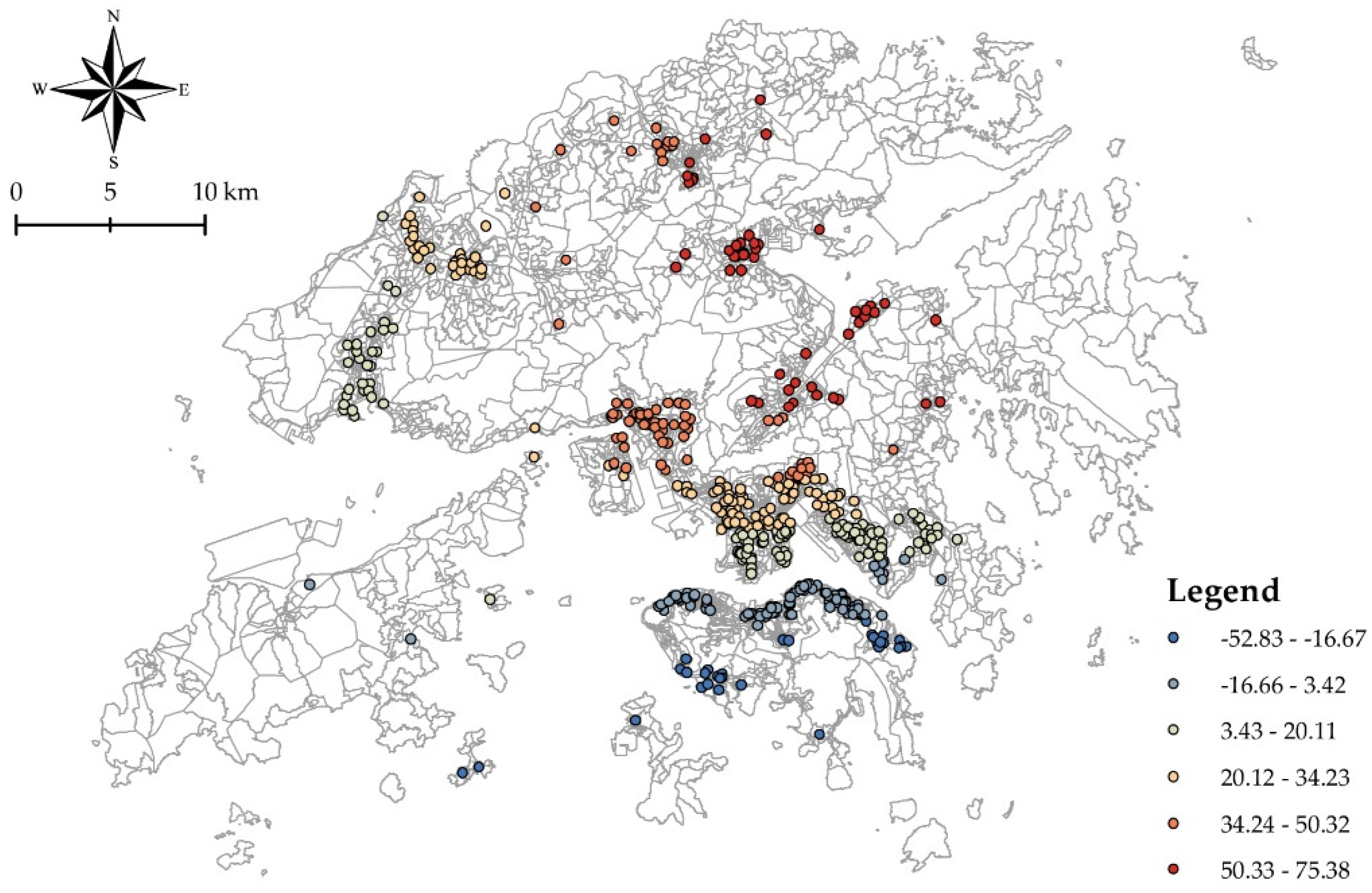
Street greenery variables have spatially nonstationary influences on walking time. For example, in GWR model 1, the variable has an unstandardized coefficient ranging from −52.83 and 75.38 (a wide range). This observation indicates that street greenery has a positive influence in some locations, but the influence turns negative in other places.
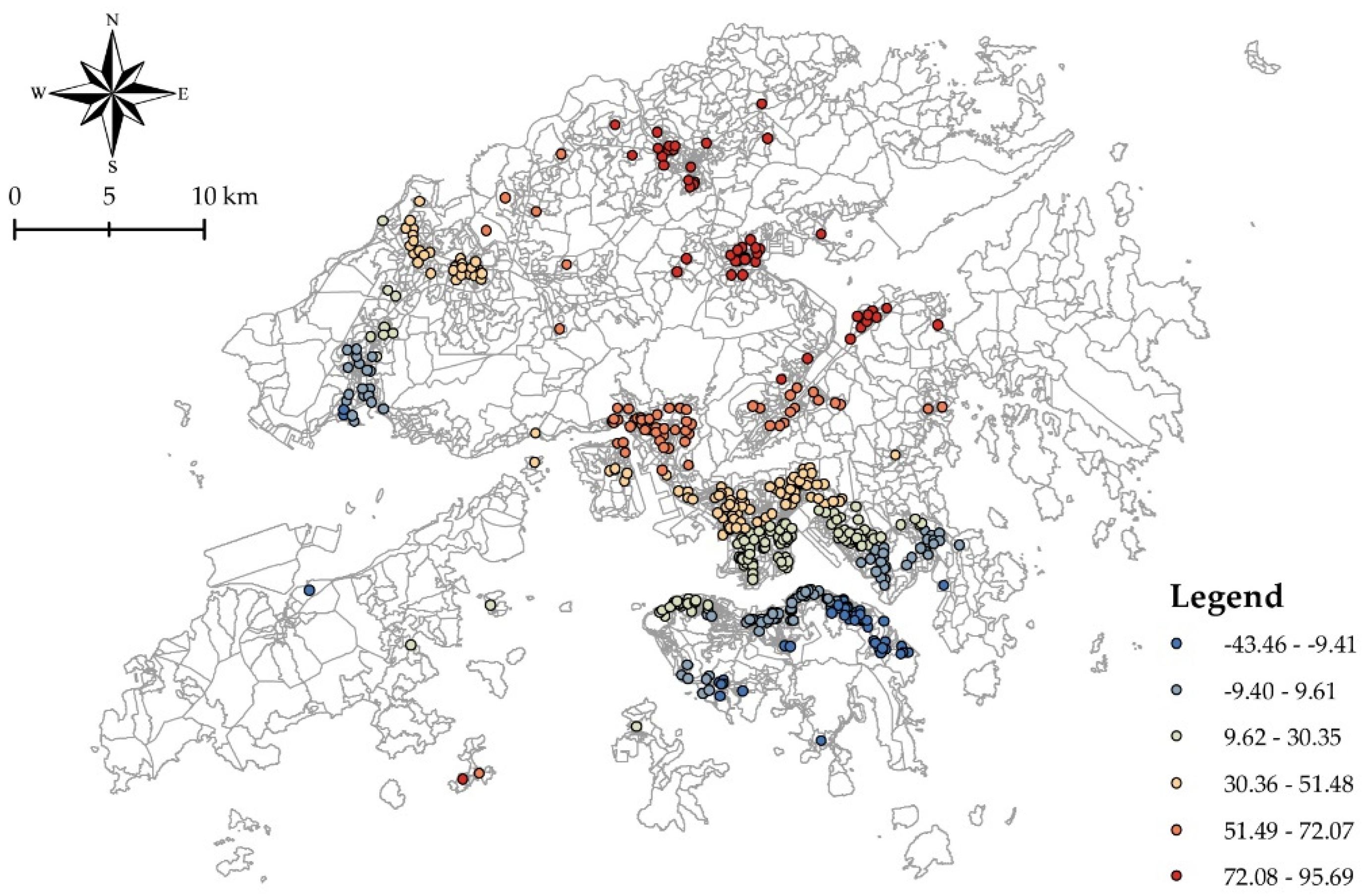
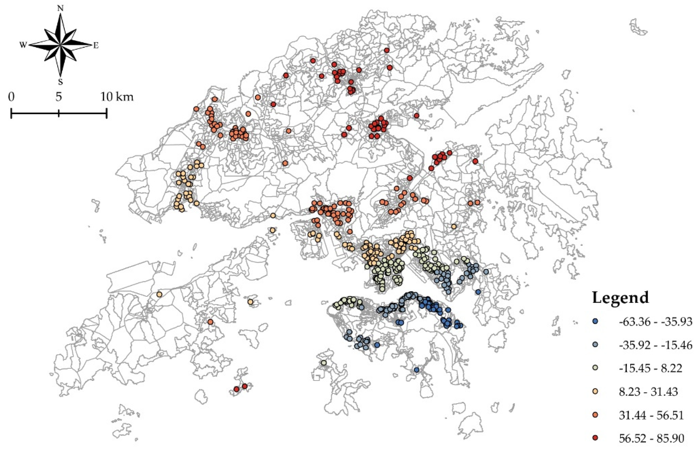
As mentioned before, an apparent strength of the GWR model is that its output can be visualized easily for a better understanding of the marginal effects of independent variables on the response variable. Figure 3, Figure 4 and Figure 5 show the geographical distribution of the coefficient of street greenery 400 m (in GWR model 1), 800 m (in GWR model 2), and 1600 m (in GWR model 3), respectively. The Jenks Natural Breaks Classification method (No. of classes = 6) is used for coefficient classification. (As previously mentioned, of particular interest is the interpretation of street greenery variables. Indeed, other variables’ coefficients can be visualized as well. The visualization outcomes can be obtained from the corresponding author upon reasonable request.)
Street greenery variables behave highly consistently in the three GWR models. Moran’s I tests (with 99,999 permutations) are conducted in GeoDa (Version 1.14) to detect the existence of spatial autocorrelation (spatial dependence). The results illustrate the presence of spatial autocorrelation in the coefficient of street greenery in all three GWR models. We find that low clusters are located in the south of the city, indicating that street greenery has a lower walking time-uplifting effect in the urban area, namely Hong Kong Island and Kowloon. In other words, in the suburban area (the New Territories), older adults have a higher predilection for street greenery. This finding is congruent with Yang et al. [44], which exclusively focuses on travel propensity (another mobility measure). A possible explanation is that people with low income (who usually live in the suburban area) have a higher preference for street greenery and are thus more likely to walk out given the same amount of street greenery in the neighborhood [49]. There are, however, other alternative explanations.
6. Discussion
6.1. Implications for Research
Notably, this study exclusively uses GSV data to estimate the green view index because its main focus is street greenery, a hypothesized essential and easily perceived contributor to older adults’ walking time (partially due to biophilia, people’s innate affinity). Hence, this study exclusively detects and extracts visual features (specifically, greenery) from street view imagery. However, street view imagery has considerably greater potential to represent the urban physical environment. As Kang et al. [14] suggest, by using street view imagery data, we can objectively represent the “elements” and “scenes” of the built environment. The former provides low-level semantic information, whereas the latter offers high-level information. Other than greenery, more visual features can be detected and extracted from street view imagery at the element level. Such features include but are not limited to the sky, water bodies, traffic signs, smoke-free signage, and zebra crosswalks [32]. Therefore, more factors, such as sky view factor and street canyons, can be accurately calculated in future travel studies. Focusing on the entire scene and discovering the underlying semantics become the research aim at the scene level. Deep learning algorithms are always used in such research [14].
Street view imagery has great potential in urban physical environmental studies to enhance our understanding of many issues. Thus, it can supplement but definitely cannot fully replace traditional data acquisition methods, such as questionnaire surveys, self-reports, field audits, and remote sensing. Indeed, these data sources capture the urban physical environment from totally different dimensions. A single data source cannot fully describe the urban physical environment, and no data sources can dominate urban physical environmental research. We, however, agree that different data sources can be integrated and jointly used in urban studies. Such an endeavor can substantially present us with a broader picture and enhance our understanding of the world. Moreover, we suggest that the research with varying aims can choose the most appropriate data source. Small data are still well-suited to address many interesting research questions.
6.2. Implications for Practice
Generally, human-centric urban planning must follow the evidence on how people behave (e.g., walk). In other words, people’s behavior and preferences should be carefully considered in human-centric urban planning [50,51]. This study lays the foundation for evidence-based built environment planning and informs urban planners/designers to plan/design cities with an adequate level of street greenery, which is one of its practical implications. Specifically, as the findings of this study reveal that street greenery plays a critical role in the walking time determination process, street greenery should be considered in built environment planning, especially in the era with the goals of healthy and active aging. Moreover, this study offers the basis for implementing spatially varying greenery provision schemes, which is another practical implication.
In addition to street greenery (attribute of our predominant interest), many built environment attributes can be altered to change older adults’ walking behavior. As Wang et al. [52] indicated, two directions to enhance a place’s walkability and encourage people’s walking behavior are (1) providing a safe, comfortable, pleasant, and continuous walking environment (assuring “how to walk” from a physical perspective) and (2) locating various opportunities within (reasonable) walking distance (assuring “why to walk” from a functional perspective). However, the opportunities for older adults are vastly different from those for younger adults. We will discuss this argument and related conventional thinking in detail as follows.
Travel demand is normally perceived as a derived demand [34]. That is, residents rarely travel for the pleasure of movement but make journeys to reach the opportunities available at destinations. To some extent, this situation is true for younger adults, who have limited free time and often make mandatory trips (the purpose of most of their trips is accessing opportunities rather than recreation and leisure.). However, we conjecture that the above argument cannot be applied to older adults—a cohort with considerable free time. Older adults make few mandatory trips (e.g., commuting and going to school) but many discretionary trips. They may pay little attention to built environment attributes related to the opportunities highly regarded by younger adults (e.g., workplaces, schools, bars, gyms, sports centers, and museums) [53,54]. For example, in China, in older adults’ eyes, opportunities may include chess/card rooms, urban parks, open spaces, and vegetable markets [53,54]. Therefore, we appeal to elderly travel researchers to carefully choose built environment attributes, especially those highly relevant to opportunities.
Accessibility, generally defined as the ease of reaching opportunities, is a transportation–land use planning goal [55]. Therefore, in accessibility planning (or transportation–land-use planning), the accurate selection of the indicators truly characterizing proper opportunities in the view of older adults is indispensable.
6.3. Research limitations
Despite offering many interesting findings, this study is by no means free from limitations. First, the empirical data used in this study are cross-sectional. Therefore, it fails to determine the causality between street greenery and older adults’ walking behavior. In other words, the residential self-selection issue cannot be eliminated, although it is not serious for older adults (who have limited freedom for residential relocation) [31]. Admittedly, conducting a before-and-after study in the future can help establish a causal relationship and obtain stronger conclusions.
Second, due to the TCS 2011 data limitations that cannot be remedied by us, many potential predictors of walking behavior, such as attitudes, long-established preferences, habits, and weather, cannot be modeled. Hence, designing and conducting a survey to collect first-hand data on more aspects of individuals, trips, or weather is necessary for future fine-grained studies. Moreover, a time gap between walking behavior evaluation and street greenery assessment may exist.
Third, we identify a spatial pattern of the marginal effect of street greenery. Based on scatter evidence in the existing literature, we suspect but cannot conclude that the above finding can be attributable to differences in socioeconomic statuses (specifically, income). We cannot rule out other explanations (e.g., a lower density of recreational facilities is the source) simply based on the GWR modeling results. This is an inherent disadvantage of the GWR model, which can well reveal a spatial pattern but cannot be used for hypothesis testing.
Fourth, this study solely focuses on one walking behavior measure: walking time. Other measures, such as walking propensity, walking trip frequency, transportation walking propensity, and recreational walking frequency, can be investigated in future research.
Fifth, this study only identifies the “global” and “local” effect of street greenery on older adults’ walking time. More sophisticated studies on the basis of advanced techniques, such as random forest, multiple additive regression trees, and AdaBoost decision tree, should be conducted to reveal the complex relationship between street greenery and the walking behavior of older adults.
Last but not least, this study offers strong evidence supporting significant associations between street greenery and the walking time of older adults. A question arises: why does street greenery affect people’s walking time (more broadly, physical activity)? This study cannot reject the claim that street greenery is a proxy for further variables that support walking but are not explicitly considered here. More detailed and micro-scale studies are needed to study the mechanism through which street greenery affects people’s walking time. Therefore, we appeal to researchers worldwide, for example, those from psychology and psychometrics fields, to pay substantial attention to the link between greenery and physical activity and identify possible mediators through methodologically rigorous research design.
7. Conclusions
Hong Kong is facing a population aging problem, and older populations will keep increasing in the forthcoming years. In view of the importance of walking for healthy and active aging, researchers should constantly agitate for a highly walkable city (and places with high walkability). Analyzing the correlates of older adults’ walking behavior is a prerequisite for creating an elderly-friendly and walkable city.
This study elucidates street greenery as a contributor to the walking time of older adults. In a department from previous studies solely focusing on the global or average effect, this study analyzes the spatial heterogeneity in such an effect using GWR models. Moreover, street greenery is evaluated in neighborhoods of different sizes (400 m, 800 m, and 1600 m). This study concludes that the influence of street greenery on the walking time of older adults varies across space. Specifically, it is greater in the suburban area.
Author Contributions
Conceptualization, Linchuan Yang and Jixiang Liu; methodology, Linchuan Yang; software, Yuan Liang; validation, Jixiang Liu, Yi Lu, and Hongtai Yang; formal analysis, Yuan Liang; investigation, Linchuan Yang and Yuan Liang; resources, Linchuan Yang; data curation, Linchuan Yang and Yi Lu; writing—original draft preparation, Linchuan Yang and Jixiang Liu; writing—review and editing, Yuan Liang, Yi Lu, and Hongtai Yang; visualization, Linchuan Yang and Jixiang Liu; supervision, Linchuan Yang; project administration, Linchuan Yang; funding acquisition, Linchuan Yang. All authors have read and agreed to the published version of the manuscript.
Funding
This research was supported by the Research Fund from Sichuan Rural Community Governance Research Center (No. SQZL2021B03) and the Fundamental Research Funds for the Central Universities of China (No. 2682021CX097 and No. 2682021ZTPY111).
Institutional Review Board Statement
Not applicable.
Informed Consent Statement
Not applicable.
Data Availability Statement
The data are available from the corresponding author upon reasonable request.
Acknowledgments
The authors are grateful to the four reviewers for their constructive comments.
Conflicts of Interest
The authors declare no conflict of interest. The funders had no role in the design of the study; in the collection, analyses, or interpretation of data; in the writing of the manuscript, or in the decision to publish the results.
Appendix A

Table A1.
Box–Cox transformation modeling results.
| Variable | Model 4 | Model 5 | Model 6 |
|---|---|---|---|
| Coef. | Coef. | Coef. | |
| Street greenery (400 m) | 0.023 *** | ||
| Street greenery (800 m) | 0.017 *** | ||
| Street greenery (1600 m) | 0.014 *** | ||
| Performance statistic | |||
| Log-likelihood | −3584.56 | −3595.46 | −3595.45 |
| AIC | 7173.13 | 7192.92 | 7192.90 |
Note: *** p < 0.01. The parameter estimates of control variables are largely consistent with those in linear regression models and thus are not presented for brevity.
References
- Harper, S. Economic and social implications of aging societies. Science 2014, 346, 587–591. [Google Scholar] [CrossRef] [PubMed]
- Bao, Z.; Lee, W.M.; Lu, W. Implementing on-site construction waste recycling in Hong Kong: Barriers and facilitators. Sci. Total Environ. 2020, 747, 141091. [Google Scholar] [CrossRef]
- Census and Statistics Department. Hong Kong Population Projections 2020–2069; Hong Kong SAR Government: Hong Kong, 2020.
- Smarzaro, R.; Davis, C.A.; Quintanilha, J.A. Creation of a multimodal urban transportation network through spatial data integration from authoritative and crowdsourced data. ISPRS Int. J. Geo-Inf. 2021, 10, 470. [Google Scholar] [CrossRef]
- Alsnih, R.; Hensher, D.A. The mobility and accessibility expectations of seniors in an aging population. Transp. Res. Part A Policy Pract. 2003, 37, 903–916. [Google Scholar] [CrossRef]
- Su, F.; Bell, M.G. Transport for older people: Characteristics and solutions. Res. Transp. Econ. 2009, 25, 46–55. [Google Scholar] [CrossRef]
- Cheng, L.; Chen, X.; Yang, S.; Cao, Z.; De Vos, J.; Witlox, F. Active travel for active ageing in China: The role of built environment. J. Transp. Geogr. 2019, 76, 142–152. [Google Scholar] [CrossRef]
- Heath, G.W.; Parra, D.C.; Sarmiento, O.L.; Andersen, L.B.; Owen, N.; Goenka, S.; Montes, F.; Brownson, R.C.; Lancet Physical Activity Series Working Group. Evidence-based intervention in physical activity: Lessons from around the world. Lancet 2012, 380, 272–281. [Google Scholar] [CrossRef] [Green Version]
- Bauman, A.E.; Reis, R.S.; Sallis, J.F.; Wells, J.C.; Loos, R.J.; Martin, B.W.; Group, L.P.A.S.W. Correlates of physical activity: Why are some people physically active and others not? Lancet 2012, 380, 258–271. [Google Scholar] [CrossRef]
- Yang, H.; Liang, Y.; Yang, L. Equitable? Exploring ridesourcing waiting time and its determinants. Transp. Res. Part D Transp. Environ. 2021, 93, 102774. [Google Scholar] [CrossRef]
- Li, W.; Zhu, J.; Fu, L.; Zhu, Q.; Guo, Y.; Gong, Y. A rapid 3D reproduction system of dam-break floods constrained by post-disaster information. Environ. Model. Softw. 2021, 139, 104994. [Google Scholar] [CrossRef]
- Li, W.; Zhu, J.; Fu, L.; Zhu, Q.; Xie, Y.; Hu, Y. An augmented representation method of debris flow scenes to improve public perception. Int. J. Geogr. Inf. Sci. 2021, 35, 1521–1544. [Google Scholar] [CrossRef]
- Liu, X.; Wang, X.; Wright, G.; Cheng, J.C.; Li, X.; Liu, R. A state-of-the-art review on the integration of Building Information Modeling (BIM) and Geographic Information System (GIS). ISPRS Int. J. Geo-Inf. 2017, 6, 53. [Google Scholar] [CrossRef] [Green Version]
- Kang, Y.; Zhang, F.; Gao, S.; Lin, H.; Liu, Y. A review of urban physical environment sensing using street view imagery in public health studies. Ann. GIS 2020, 26, 261–275. [Google Scholar] [CrossRef]
- Xue, F.; Li, X.; Lu, W.; Webster, C.J.; Chen, Z.; Lin, L. Big Data-Driven Pedestrian Analytics: Unsupervised Clustering and Relational Query Based on Tencent Street View Photographs. ISPRS Int. J. Geo-Inf. 2021, 10, 561. [Google Scholar] [CrossRef]
- Cheng, L.; Shi, K.; De Vos, J.; Cao, M.; Witlox, F. Examining the spatially heterogeneous effects of the built environment on walking among older adults. Transp. Policy 2020, 100, 21–30. [Google Scholar] [CrossRef]
- Yang, H.; Zhang, Y.; Zhong, L.; Zhang, X.; Ling, Z. Exploring spatial variation of bike sharing trip production and attraction: A study based on Chicago’s Divvy system. Appl. Geogr. 2020, 115, 102130. [Google Scholar] [CrossRef]
- Cerin, E.; Nathan, A.; Van Cauwenberg, J.; Barnett, D.W.; Barnett, A. The neighbourhood physical environment and active travel in older adults: A systematic review and meta-analysis. Int. J. Behav. Nutr. Phys. Act. 2017, 14, 15. [Google Scholar] [CrossRef] [Green Version]
- Van Cauwenberg, J.; De Bourdeaudhuij, I.; De Meester, F.; Van Dyck, D.; Salmon, J.; Clarys, P.; Deforche, B. Relationship between the physical environment and physical activity in older adults: A systematic review. Health Place 2011, 17, 458–469. [Google Scholar] [CrossRef]
- Yang, Y.; He, D.; Gou, Z.; Wang, R.; Liu, Y.; Lu, Y. Association between street greenery and walking behavior in older adults in Hong Kong. Sustain. Cities Soc. 2019, 51, 101747. [Google Scholar] [CrossRef]
- Procter-Gray, E.; Leveille, S.G.; Hannan, M.T.; Cheng, J.; Kane, K.; Li, W. Variations in community prevalence and determinants of recreational and utilitarian walking in older age. J. Aging Res. 2015, 2015, 382703. [Google Scholar] [CrossRef] [Green Version]
- Chudyk, A.M.; McKay, H.A.; Winters, M.; Sims-Gould, J.; Ashe, M.C. Neighborhood walkability, physical activity, and walking for transportation: A cross-sectional study of older adults living on low income. BMC Geriatr. 2017, 17, 82. [Google Scholar] [CrossRef] [PubMed]
- Leung, K.M.; Chung, P.-K.; Wang, D.; Liu, J.D. Impact of physical and social environments on the walking behaviour of Hong Kong’s older adults. J. Transp. Health 2018, 9, 299–308. [Google Scholar] [CrossRef]
- Liu, J.; Wang, B.; Xiao, L. Non-linear associations between built environment and active travel for working and shopping: An extreme gradient boosting approach. J. Transp. Geogr. 2021, 92, 103034. [Google Scholar] [CrossRef]
- Shigematsu, R.; Sallis, J.F.; Conway, T.L.; Saelens, B.E.; Frank, L.D.; Cain, K.L.; Chapman, J.E.; King, A.C. Age differences in the relation of perceived neighborhood environment to walking. Med. Sci. Sports Exerc. 2009, 41, 314. [Google Scholar] [CrossRef]
- Yang, L.; Ao, Y.; Ke, J.; Lu, Y.; Liang, Y. To walk or not to walk? Examining non-linear effects of streetscape greenery on walking propensity of older adults. J. Transp. Geogr. 2021, 94, 103099. [Google Scholar] [CrossRef]
- Zang, P.; Liu, X.; Zhao, Y.; Guo, H.; Lu, Y.; Xue, C.Q. Eye-level street greenery and walking behaviors of older adults. Int. J. Environ. Res. Public Health 2020, 17, 6130. [Google Scholar] [CrossRef] [PubMed]
- Zang, P.; Lu, Y.; Ma, J.; Xie, B.; Wang, R.; Liu, Y. Disentangling residential self-selection from impacts of built environment characteristics on travel behaviors for older adults. Soc. Sci. Med. 2019, 238, 112515. [Google Scholar] [CrossRef]
- Handy, S.; Cao, X.; Mokhtarian, P.L. Self-selection in the relationship between the built environment and walking: Empirical evidence from Northern California. J. Am. Plan. Assoc. 2006, 72, 55–74. [Google Scholar] [CrossRef]
- Larrañaga, A.M.; Rizzi, L.I.; Arellana, J.; Strambi, O.; Cybis, H.B.B. The influence of built environment and travel attitudes on walking: A case study of Porto Alegre, Brazil. Int. J. Sustain. Transp. 2016, 10, 332–342. [Google Scholar] [CrossRef]
- Cheng, L.; De Vos, J.; Shi, K.; Yang, M.; Chen, X.; Witlox, F. Do residential location effects on travel behavior differ between the elderly and younger adults? Transp. Res. Part D Transp. Environ. 2019, 73, 367–380. [Google Scholar] [CrossRef]
- Biljecki, F.; Ito, K. Street view imagery in urban analytics and GIS: A review. Landsc. Urban Plan. 2021, 215, 104217. [Google Scholar] [CrossRef]
- Long, J.; Shelhamer, E.; Darrell, T. Fully convolutional networks for semantic segmentation. In Proceedings of the IEEE Conference on Computer Vision and Pattern Recognition, Boston, MA, USA, 7–12 June 2015; pp. 3431–3440. [Google Scholar]
- Cervero, R.; Kockelman, K. Travel demand and the 3Ds: Density, diversity, and design. Transp. Res. Part D Transp. Environ. 1997, 2, 199–219. [Google Scholar] [CrossRef]
- Ewing, R.; Cervero, R. Travel and the built environment: A meta-analysis. J. Am. Plan. Assoc. 2010, 76, 265–294. [Google Scholar] [CrossRef]
- Osborne, J. Improving your data transformations: Applying the Box-Cox transformation. Pract. Assess. Res. Eval. 2010, 15, 12. [Google Scholar]
- Fotheringham, A.S.; Brunsdon, C.; Charlton, M. Geographically Weighted Regression: The Analysis of Spatially Varying Relationships; John Wiley & Sons: Chichester, UK, 2002. [Google Scholar]
- Tang, J.; Gao, F.; Han, C.; Cen, X.; Li, Z. Uncovering the spatially heterogeneous effects of shared mobility on public transit and taxi. J. Transp. Geogr. 2021, 95, 103134. [Google Scholar] [CrossRef]
- Xuan, W.; Zhang, F.; Zhou, H.; Du, Z.; Liu, R. Improving geographically weighted regression considering directional nonstationary for ground-Level PM2.5 estimation. ISPRS Int. J. Geo-Inf. 2021, 10, 413. [Google Scholar] [CrossRef]
- Zhao, R.; Zhan, L.; Yao, M.; Yang, L. A geographically weighted regression model augmented by Geodetector analysis and principal component analysis for the spatial distribution of PM2.5. Sustain. Cities Soc. 2020, 56, 102106. [Google Scholar] [CrossRef]
- Tobler, W.R. A computer movie simulating urban growth in the Detroit region. Econ. Geogr. 1970, 46, 234–240. [Google Scholar] [CrossRef]
- Xu, P.; Huang, H. Modeling crash spatial heterogeneity: Random parameter versus geographically weighting. Accid. Anal. Prev. 2015, 75, 16–25. [Google Scholar] [CrossRef]
- Pan, R.; Yang, H.; Xie, K.; Wen, Y. Exploring the equity of traditional and ride-hailing taxi services during peak hours. Transp. Res. Rec. 2020, 2674, 266–278. [Google Scholar] [CrossRef]
- Yang, L.; Liu, J.; Lu, Y.; Ao, Y.; Guo, Y.; Huang, W.; Zhao, R.; Wang, R. Global and local associations between urban greenery and travel propensity of older adults in Hong Kong. Sustain. Cities Soc. 2020, 63, 102442. [Google Scholar] [CrossRef]
- Liu, J.; Shi, W. A cross-boundary travel tale: Unraveling Hong Kong residents’ mobility pattern in Shenzhen by using metro smart card data. Appl. Geogr. 2021, 130, 102416. [Google Scholar] [CrossRef]
- Feng, J.; Dijst, M.; Wissink, B.; Prillwitz, J. The impacts of household structure on the travel behaviour of seniors and young parents in China. J. Transp. Geogr. 2013, 30, 117–126. [Google Scholar] [CrossRef]
- Saelens, B.E.; Sallis, J.F.; Frank, L.D. Environmental correlates of walking and cycling: Findings from the transportation, urban design, and planning literatures. Ann. Behav. Med. 2003, 25, 80–91. [Google Scholar] [CrossRef] [PubMed]
- Cerin, E.; Lee, K.-Y.; Barnett, A.; Sit, C.H.; Cheung, M.-C.; Chan, W.-M. Objectively-measured neighborhood environments and leisure-time physical activity in Chinese urban elders. Prev. Med. 2013, 56, 86–89. [Google Scholar] [CrossRef]
- James, P.; Banay, R.F.; Hart, J.E.; Laden, F. A review of the health benefits of greenness. Curr. Epidemiol. Rep. 2015, 2, 131–142. [Google Scholar] [CrossRef] [PubMed] [Green Version]
- Jing, C.; Bryan-Kinns, N.; Yang, S.; Zhi, J.; Zhang, J. The influence of mobile phone location and screen orientation on driving safety and the usability of car-sharing software in-car use. Int. J. Ind. Ergon. 2021, 84, 103168. [Google Scholar] [CrossRef]
- Bao, Z.; Lu, W.; Hao, J. Tackling the “last mile” problem in renovation waste management: A case study in China. Sci. Total Environ. 2021, 790, 148261. [Google Scholar] [CrossRef]
- Wang, H.; Huang, J.; Li, Y.; Yan, X.; Xu, W.A. Evaluating and mapping the walking accessibility, bus availability and car dependence in urban space: A case study of Xiamen, China. Acta Geogr. Sin. 2013, 68, 477–490. [Google Scholar]
- Feng, J. The influence of built environment on travel behavior of the elderly in urban China. Transp. Res. Part D Transp. Environ. 2017, 52, 619–633. [Google Scholar] [CrossRef]
- Cheng, L.; Caset, F.; De Vos, J.; Derudder, B.; Witlox, F. Investigating walking accessibility to recreational amenities for elderly people in Nanjing, China. Transp. Res. Part D Transp. Environ. 2019, 76, 85–99. [Google Scholar] [CrossRef]
- Handy, S.L.; Niemeier, D.A. Measuring accessibility: An exploration of issues and alternatives. Environ. Plan. A 1997, 29, 1175–1194. [Google Scholar] [CrossRef]
Figure 1.
Machine learning technique–based estimation of the green view index.

Figure 2.
The geographical distribution of the green view index in Hong Kong.

Figure 3.
Geographical distribution of the coefficient of street greenery (400 m).

Figure 4.
Geographical distribution of the coefficient of street greenery (800 m).

Figure 5.
Geographical distribution of the coefficient of street greenery (1600 m).

Table 1.
Summary of the independent variables.
| Variable | Category | Description | Mean/Percentage | Std. Dev. |
|---|---|---|---|---|
| Socioeconomic characteristics | ||||
| Family size | Number of persons in the family. Discrete variable. | 2.83 | 1.44 | |
| Male | Dummy variable. = 1 for male, = 0 for female | 0.47 | ||
| Age | Unit: year. Discrete variable. | 74.24 | 7.00 | |
| Family income | Total monthly family income (including all incomes and Mandatory Provident Fund contributions). Ordinal variable ranging from 1 (<HK $4000/month) to 19 (≥HK $150,000/month) | 6.18 | 4.49 | |
| Built environment | ||||
| Population density | Density | Neighborhood-level population density. Continuous variable (unit: 104 people/km2) | 5.08 | 3.33 |
| Land use mix | Diversity | Neighborhood-level land use entropy. Continuous variable ranging from 0 to 1 (no units). Three types of land use, including residential, office, and retail, are considered. | 0.54 | 0.27 |
| Intersection density | Design | Neighborhood-level street intersection density. Continuous variable (unit: 1/km2) | 63.82 | 28.85 |
| Access to the metro | Distance to transit | Number of metro stations within 400 m. Discrete variable. | 0.36 | 0.49 |
| Access to recreational facilities | Destination accessibility | Number of recreational facilities within 400 m. Discrete variable. | 60.99 | 28.75 |
| Street greenery (400 m) | Design | Green view index within 400 m. Continuous variable ranging from 0 to 1 (no units) | 0.15 | 0.05 |
| Street greenery (800 m) | Design | Green view index within 800 m. Continuous variable ranging from 0 to 1 (no units) | 0.15 | 0.04 |
| Street greenery (1600 m) | Design | Green view index within 1600 m. Continuous variable ranging from 0 to 1 (no units) | 0.15 | 0.04 |
| Sample size | 1083 | |||
Table 2.
Linear regression modeling results.
| Variable | Model 1 | Model 2 | Model 3 | |||
|---|---|---|---|---|---|---|
| Coef. | t-stat. | Coef. | t-stat. | Coef. | t-stat. | |
| Family size | −0.827 * | −1.70 | −0.813 * | −1.67 | −0.806 * | −1.65 |
| Male | −0.504 | −0.49 | −0.386 | −0.37 | −0.370 | −0.36 |
| Age | −0.180 ** | −2.42 | −0.185 ** | −2.50 | −0.185 ** | −2.49 |
| Family income | −0.222 | −1.42 | −0.239 | −1.53 | −0.241 | −1.54 |
| Population density | 0.322 | 1.44 | 0.373 * | 1.66 | 0.346 | 1.54 |
| Land use mix | 4.162 | 1.27 | 4.294 | 1.31 | 3.639 | 1.11 |
| Intersection density | −0.043 | −0.24 | −0.023 | −0.12 | −0.056 | −0.30 |
| Access to the metro | −0.908 | −0.81 | −0.970 | −0.87 | −1.098 | −0.98 |
| Access to recreational facilities | 0.266 *** | 4.19 | 0.293 *** | 4.58 | 0.287 *** | 4.49 |
| Street greenery (400 m) | 32.949 ** | 2.48 | ||||
| Street greenery (800 m) | 46.642 *** | 2.79 | ||||
| Street greenery (1600 m) | 37.851 ** | 2.11 | ||||
| Constant | 22.082 *** | 3.41 | 19.406 *** | 2.87 | 21.363 *** | 3.13 |
| Performance statistic | ||||||
| Log-likelihood | −4592.63 | −4591.80 | −4593.48 | |||
| AIC | 9207.25 | 9205.61 | 9208.97 | |||
| AICc | 9209.54 | 9207.90 | 9211.26 | |||
Note: *** p < 0.01; ** p < 0.05; * p < 0.1. The variable of primary interest is shown in bold.
Table 3.
GWR modeling results.
| Variable | Coef. | ||||
|---|---|---|---|---|---|
| Mean | Std. Dev. | Min | Median | Max | |
| GWR model 1 | |||||
| Family size | −0.96 | 0.26 | −1.64 | −1.04 | −0.00 |
| Male | −0.27 | 0.45 | −2.10 | −0.24 | 0.49 |
| Age | −0.21 | 0.04 | −0.28 | −0.22 | 0.11 |
| Family income | −0.17 | 0.08 | −0.43 | −0.16 | 0.13 |
| Population density | 0.27 | 0.42 | −0.33 | 0.13 | 1.31 |
| Land use mix | 3.38 | 3.18 | −2.19 | 2.79 | 9.85 |
| Intersection density | −0.01 | 0.11 | −0.42 | 0.01 | 0.40 |
| Access to the metro | −1.07 | 0.68 | −4.08 | −0.90 | 0.26 |
| Access to recreational facilities | 0.23 | 0.03 | 0.17 | 0.22 | 0.35 |
| Street greenery (400 m) | 21.10 | 23.42 | −52.83 | 21.84 | 75.38 |
| Constant | 27.14 | 6.07 | 13.03 | 28.19 | 39.86 |
| Performance statistic | |||||
| Log-likelihood | −4570.43 | ||||
| AIC | 9198.06 | ||||
| AICc | 9199.67 | ||||
| GWR model 2 | |||||
| Family size | −0.96 | 0.27 | −1.70 | −1.04 | 0.03 |
| Male | −0.19 | 0.40 | −2.28 | −0.16 | 0.53 |
| Age | −0.21 | 0.04 | −0.30 | −0.22 | 0.14 |
| Family income | −0.18 | 0.08 | −0.43 | −0.16 | 0.08 |
| Population density | 0.29 | 0.46 | −0.31 | 0.13 | 1.46 |
| Land use mix | 3.42 | 3.41 | −1.88 | 2.53 | 10.56 |
| Intersection density | 0.02 | 0.11 | −0.45 | 0.03 | 0.45 |
| Access to the metro | −1.14 | 0.68 | −3.79 | −1.06 | 1.11 |
| Access to recreational facilities | 0.24 | 0.05 | 0.17 | 0.22 | 0.41 |
| Street greenery (800 m) | 30.23 | 30.16 | −43.46 | 29.81 | 95.69 |
| Constant | 25.56 | 7.12 | 2.25 | 26.98 | 38.26 |
| Performance statistic | |||||
| Log-likelihood | −4568.26 | ||||
| AIC | 9195.47 | ||||
| AICc | 9197.18 | ||||
| GWR model 3 | |||||
| Family size | −0.94 | 0.26 | −1.46 | −1.02 | 0.03 |
| Male | −0.20 | 0.38 | −2.05 | −0.19 | 0.52 |
| Age | −0.21 | 0.04 | −0.29 | −0.21 | 0.11 |
| Family income | −0.18 | 0.08 | −0.41 | −0.16 | 0.03 |
| Population density | 0.26 | 0.46 | −0.33 | 0.10 | 1.48 |
| Land use mix | 3.07 | 3.14 | −1.11 | 2.01 | 9.81 |
| Intersection density | −0.04 | 0.11 | −0.34 | −0.04 | 0.45 |
| Access to the metro | −1.27 | 0.78 | −4.38 | −1.15 | 1.11 |
| Access to recreational facilities | 0.24 | 0.05 | 0.18 | 0.22 | 0.36 |
| Street greenery (1600 m) | 12.18 | 33.87 | −63.36 | 17.27 | 85.90 |
| Constant | 28.73 | 8.38 | 4.05 | 31.10 | 40.95 |
| Performance statistic | |||||
| Log-likelihood | −4570.83 | ||||
| AIC | 9199.12 | ||||
| AICc | 9200.75 | ||||
Note: The variable of primary interest is shown in bold.
Publisher’s Note: MDPI stays neutral with regard to jurisdictional claims in published maps and institutional affiliations. |
© 2021 by the authors. Licensee MDPI, Basel, Switzerland. This article is an open access article distributed under the terms and conditions of the Creative Commons Attribution (CC BY) license (https://creativecommons.org/licenses/by/4.0/).
Share and Cite
MDPI and ACS Style
Yang, L.; Liu, J.; Liang, Y.; Lu, Y.; Yang, H. Spatially Varying Effects of Street Greenery on Walking Time of Older Adults. ISPRS Int. J. Geo-Inf. 2021, 10, 596. https://doi.org/10.3390/ijgi10090596
AMA Style
Yang L, Liu J, Liang Y, Lu Y, Yang H. Spatially Varying Effects of Street Greenery on Walking Time of Older Adults. ISPRS International Journal of Geo-Information. 2021; 10(9):596. https://doi.org/10.3390/ijgi10090596
Chicago/Turabian StyleYang, Linchuan, Jixiang Liu, Yuan Liang, Yi Lu, and Hongtai Yang. 2021. "Spatially Varying Effects of Street Greenery on Walking Time of Older Adults" ISPRS International Journal of Geo-Information 10, no. 9: 596. https://doi.org/10.3390/ijgi10090596
Note that from the first issue of 2016, this journal uses article numbers instead of page numbers. See further details here.