
Whose Urban Green? Mapping and Classifying Public and Private Green Spaces in Padua for Spatial Planning Policies

 and
and 
Abstract
:1. Introduction
1.1. Green Spaces Management in Contemporary Urban Planning
1.2. Spatial Planning in Padua: Between Soil Sealing and Urban Greening
1.3. Aims of the Study
2. Data and Methods
2.1. Data Sources
2.2. Urban Green Spaces Detection
2.3. Data Validation
2.4. Urban Green Spaces Definition and Classification
2.5. Data Quality and Update Assessment
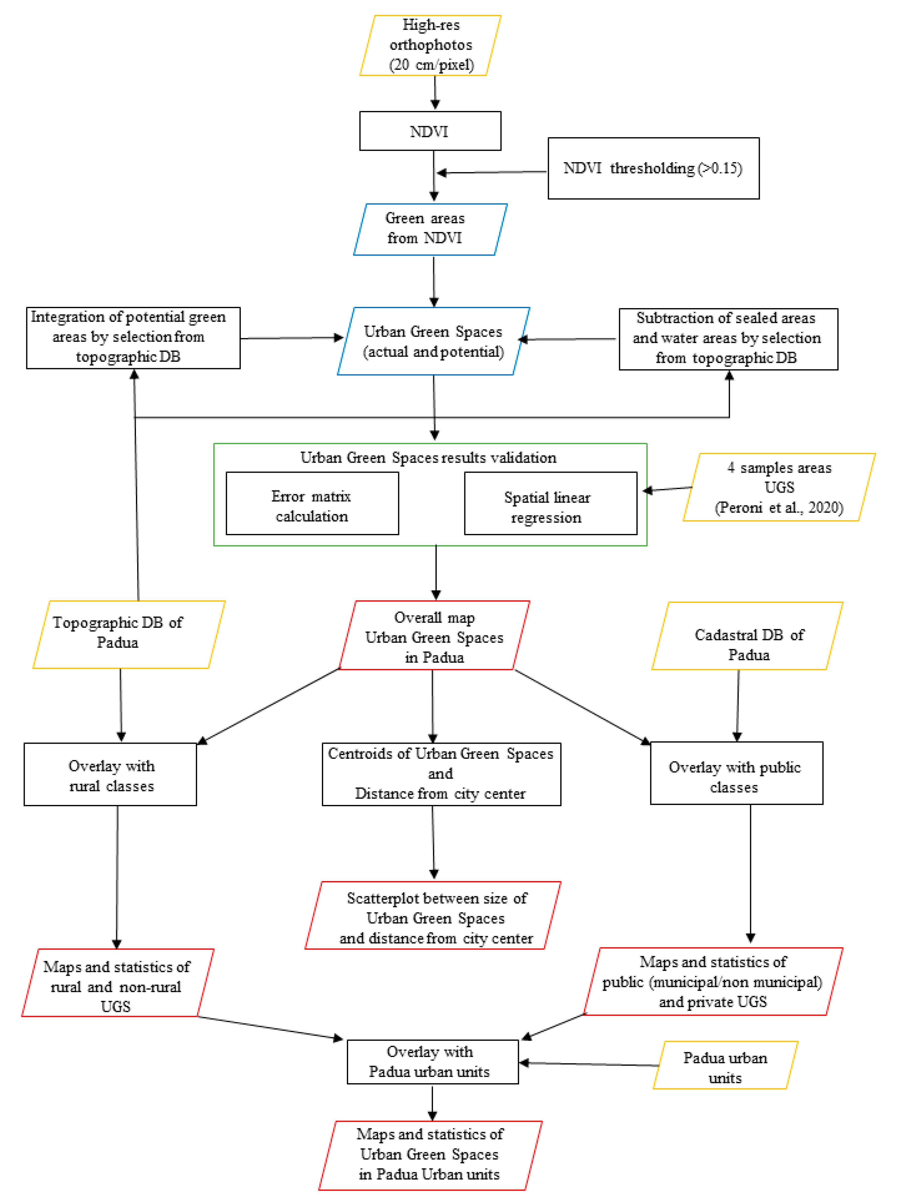
2.6. Overall Workflow
3. Results and Discussion
3.1. Urban Green Space Extraction (NDVI), Integration, and Cross Validation

| Macro-Sample Area | Green Areas from NDVI/Topo DB (km2) | Green Areas from Visual Analysis (km2) |
|---|---|---|
| Brentelle (1) | 1.84 | 1.80 |
| Forcellini (2) | 1.59 | 1.64 |
| Sacra Famiglia (3) | 1.73 | 1.71 |
| San Lazzaro (4) | 1.23 | 1.24 |
| Sample Area | R Value |
|---|---|
| Brentelle | 0.80 |
| Forcellini | 0.81 |
| Sacra Famiglia | 0.84 |
| San Lazzaro | 0.84 |
| 0 | 1 | TOTAL | PA (%) | |
|---|---|---|---|---|
| 0 | 2,785,201 | 351,455 | 3,136,656 | 84.15 |
| 1 | 524,780 | 6,870,427 | 7,395,207 | 95.13 |
| TOTAL | 3,309,981 | 7,221,882 | 10,531,863 | |
| UA (%) | 88.80 | 92.90 |
| 0 | 1 | TOTAL | PA (%) | |
|---|---|---|---|---|
| 0 | 4,899,198 | 646,442 | 5,545,640 | 91.01 |
| 1 | 484,267 | 5,864,363 | 6,348,630 | 90.07 |
| TOTAL | 5,383,465 | 6,510,805 | 11,894,270 | |
| UA (%) | 88.34 | 92.37 |
| 0 | 1 | TOTAL | PA (%) | |
|---|---|---|---|---|
| 0 | 4,382,170 | 390,491 | 4,772,661 | 89.31 |
| 1 | 524,717 | 6,323,181 | 6,847,898 | 94.18 |
| TOTAL | 4,906,887 | 6,713,672 | 11,620,559 | |
| UA (%) | 91.82 | 92.34 |
| 0 | 1 | TOTAL | PA (%) | |
|---|---|---|---|---|
| 0 | 8,320,253 | 403,748 | 8,724,001 | 93.54 |
| 1 | 574,417 | 4,359,710 | 4,934,127 | 91.52 |
| TOTAL | 8,894,670 | 4,763,458 | 13,658,128 | |
| UA (%) | 95.37 | 88.36 |
| Sample Area | Overall Accuracy (%) | Kappa Coefficient |
|---|---|---|
| Brentelle | 91.68 | 0.80 |
| Forcellini | 90.49 | 0.81 |
| Sacra Famiglia | 92.12 | 0.84 |
| San Lazzaro | 92.84 | 0.84 |
3.2. Urban Green Spaces: Estimation and Binary Classification
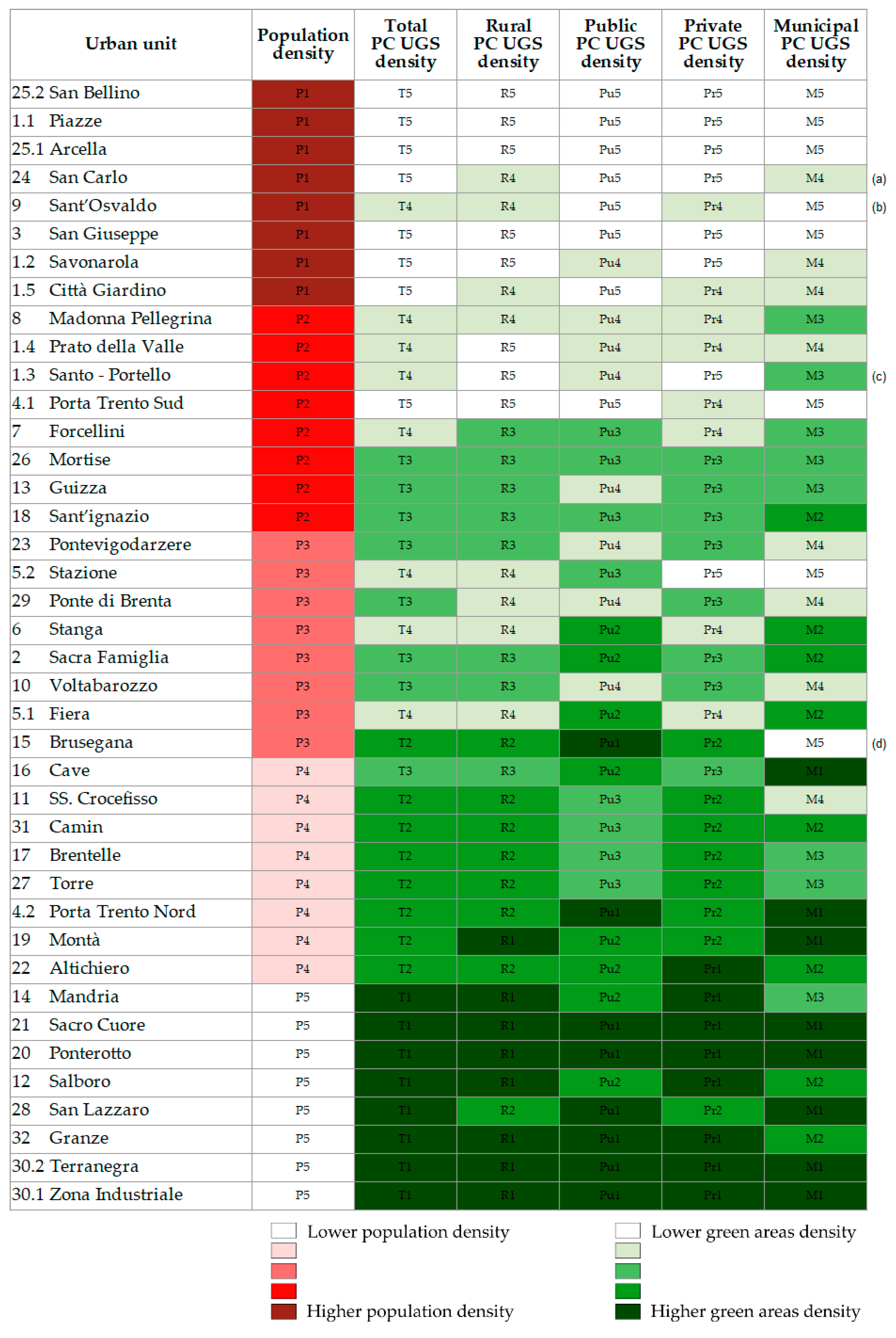
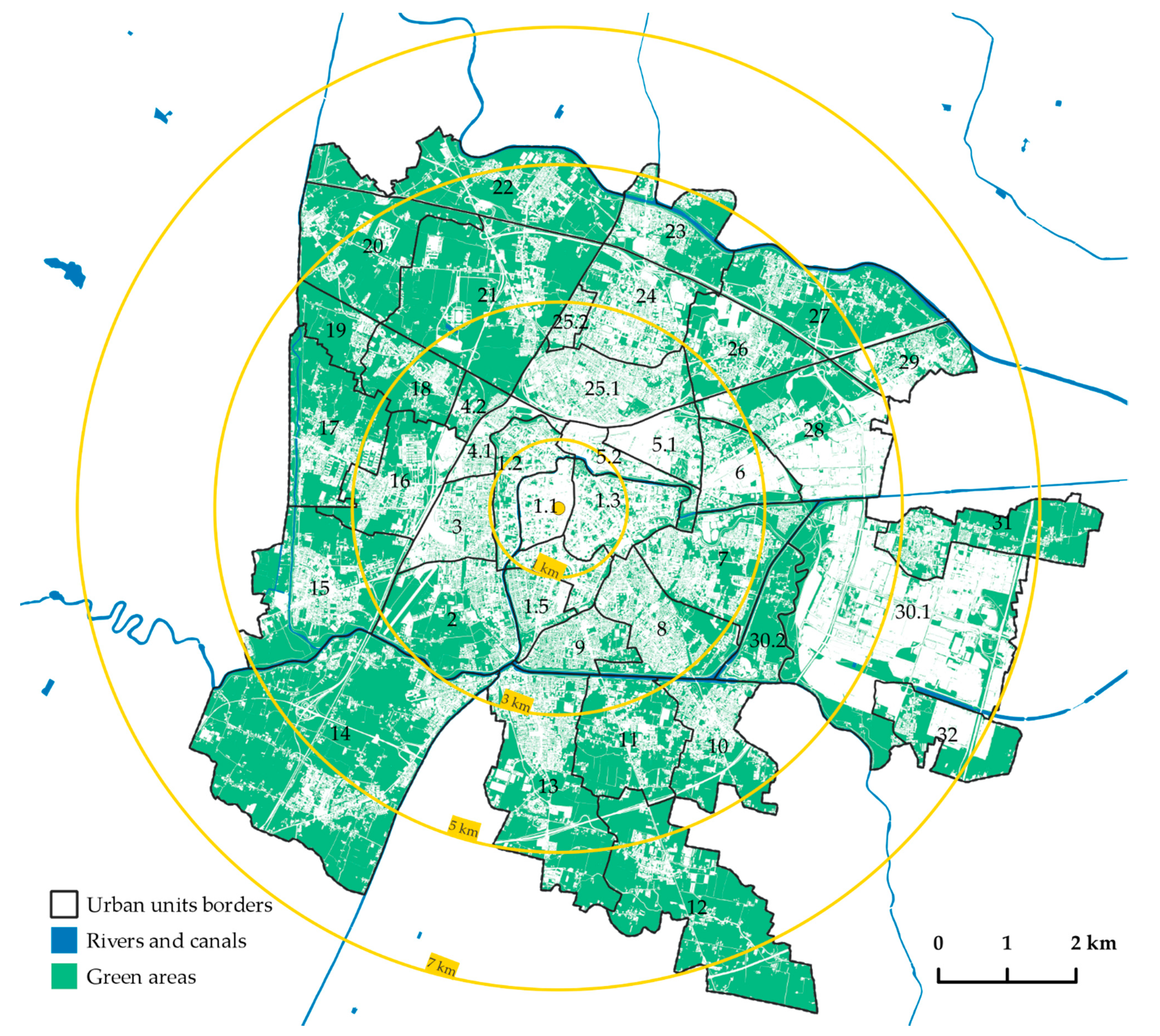
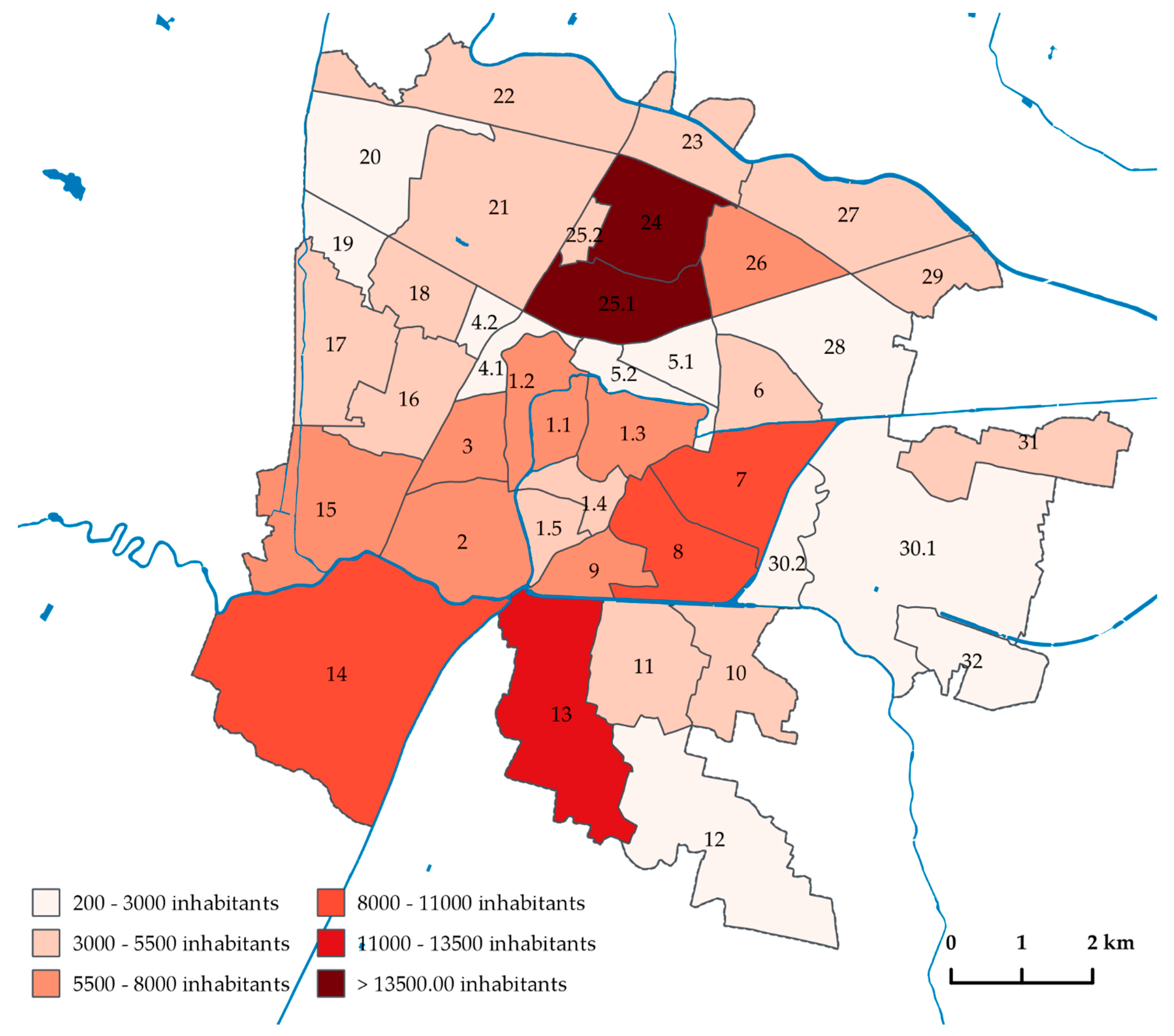
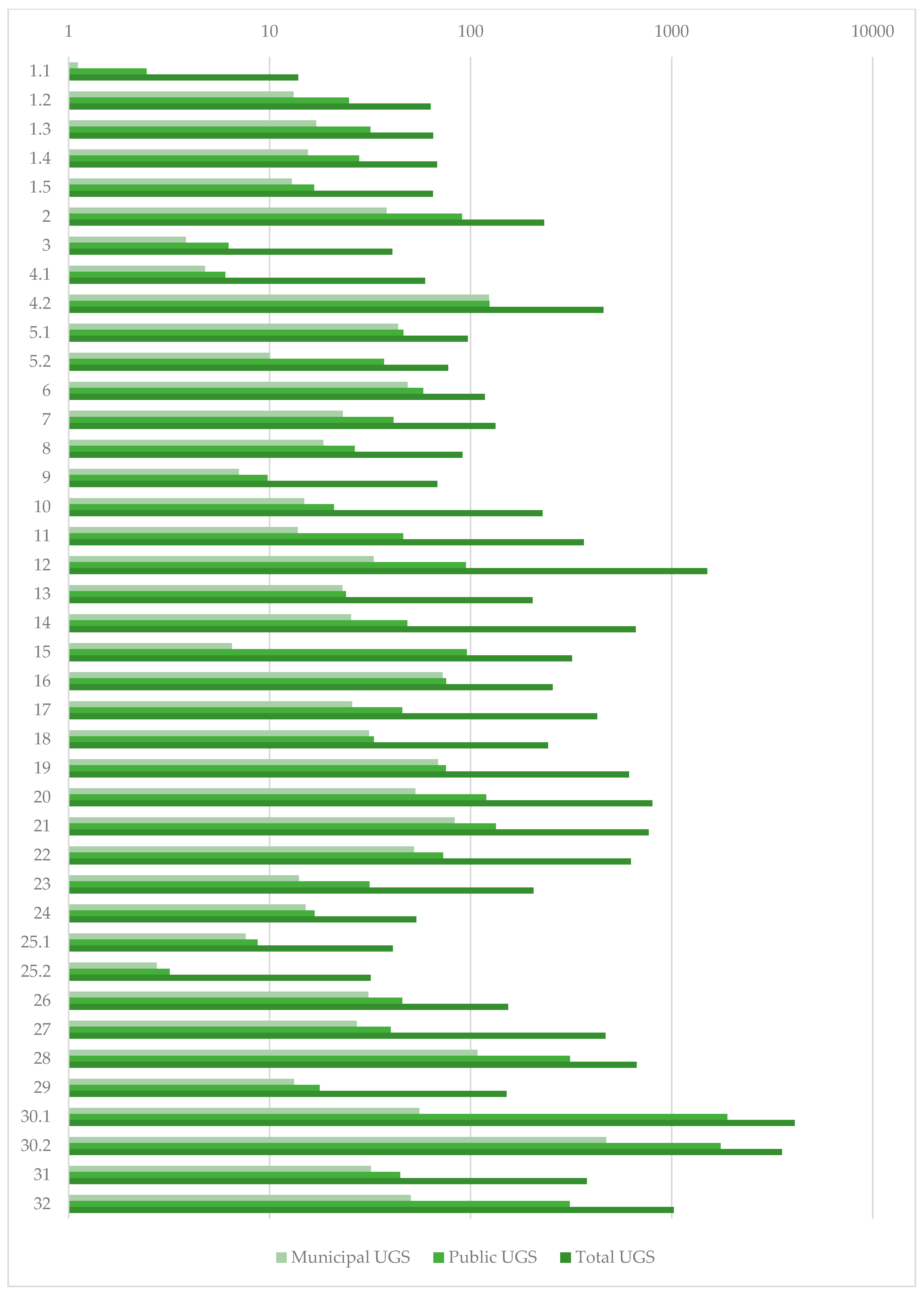
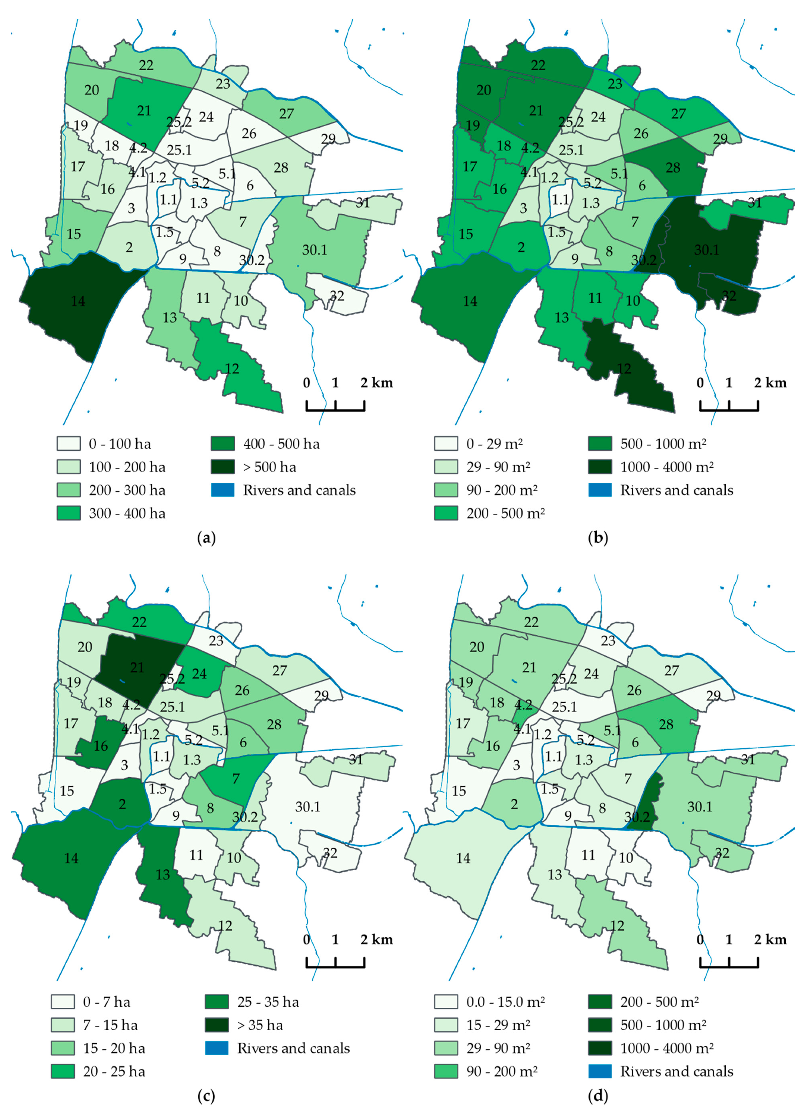
3.3. Urban Green Spaces and Population in Padua Urban Units
3.4. Urban Green Spaces: From Mapping and Classifying to Spatial Planning
4. Conclusions
Author Contributions
Funding
Data Availability Statement
Acknowledgments
Conflicts of Interest
References
- Borgström, S.; Similä, J. Integration of ecosystem services into decision-making. In Towards a Sustainable and Genuinely Green Economy. The Value and Social Significance of Ecosystem Services in Finland (TEEB for Finland) Synthesis and Roadmap; Jäppinen, J.-P., Heliölä, J., Eds.; Finland Ministry of the Environment: Helsinki, Finland, 2015; pp. 73–80. [Google Scholar]
- Colding, J. The role of ecosystem services in contemporary urban planning. In Urban Ecology: Patterns, Processes and Applications; Niemelä, J., Breuste, J.H., Elmqvist, T., Guntenspergen, G., James, P., McIntyre, N.E., Eds.; Oxford University Press: Oxford, UK, 2011; pp. 228–237. [Google Scholar]
- Cortinovis, C.; Geneletti, D. A framework to explore the effects of urban planning decisions on regulating ecosystem services in cities. Ecosyst. Serv. 2019, 38, 100946. [Google Scholar] [CrossRef]
- Davies, C.; Lafortezza, R. Transitional path to the adoption of nature-based solutions. Land Use Policy 2019, 80, 406–409. [Google Scholar] [CrossRef]
- Faivre, N.; Fritz, M.; Freitas, T.; de Boissezon, B.; Vandewoestijne, S. Nature-based solutions in the EU: Innovating with nature to address social, economic and environmental challenges. Environ. Res. 2017, 159, 509–518. [Google Scholar] [CrossRef]
- Conceptual Framework Working Group of the Millennium Ecosystem Assessment. Ecosystems and Human Well-Being. A Framework for Assessment; Island Press: Washington, DC, USA, 2003; pp. 7–19. [Google Scholar]
- Haines-Young, R.; Potschin, M. Common International Classification of Ecosystem Services (CICES): Consultation on Version 4, August–December 2012; European Environment Agency: Copenhagen, Denmark, 2013.
- Torres, A.V.; Tiwari, C.; Atkinson, S.F. Progress in ecosystem services research: A guide for scholars and practitioners. Ecosyst. Serv. 2021, 49, 101267. [Google Scholar] [CrossRef]
- Karimi, A.; Yazdandad, H.; Fagerholm, N. Evaluating social perceptions of ecosystem services, biodiversity and land management: Trade-offs, synergies and implications for landscape planning and management. Ecosyst. Serv. 2020, 45, 101188. [Google Scholar] [CrossRef]
- Hatan, S.; Fleischer, A.; Tchetchik, A. Economic valuation of cultural ecosystem services: The case of landscape aesthetics in the agritourism market. Ecol. Econ. 2021, 184, 107005. [Google Scholar] [CrossRef]
- European Commission. Mapping and Assessment of Ecosystems and Their Services. Urban Ecosystems, 4th Report–Final May 2016; Office for Official Publications of the European Communities: Luxembourg, 2016. [Google Scholar]
- Maes, J.; Zulian, G.; Günther, S.; Thijssen, M.; Raynal, J. Enhancing Resilience of Urban Ecosystems through Green Infrastructure (EnRoute) Final Report; Publications Office of the European Union: Luxembourg, 2019; ISBN 978-92-79-98984-1. [CrossRef]
- Andersson-Sköld, Y.; Klingberg, J.; Gunnarsson, B.; Cullinane, K.; Gustafsson, I.; Hedblom, M.; Knez, I.; Lindberg, F.; Sang, Å.O.; Pleijel, H.; et al. A framework for assessing urban greenery’s effects and valuing its ecosystem services. J. Environ. Manag. 2018, 205, 274–285. [Google Scholar] [CrossRef]
- Bush, J.; Doyon, A. Building urban resilience with nature-based solutions: How can urban planning contribute? Cities 2019, 95, 102483. [Google Scholar] [CrossRef]
- Xie, L.; Bulkeley, H. Nature-based solutions for urban biodiversity governance. Environ. Sci. Policy 2020, 110, 77–87. [Google Scholar] [CrossRef]
- Giachino, C.; Pattanaro, G.; Bertoldi, B.; Bollani, L.; Bonadonna, A. Nature-based solutions and their potential to attract the young generations. Land Use Policy 2021, 101, 105176. [Google Scholar] [CrossRef]
- Seiwert, A.; Rößler, S. Understanding the term green infrastructure: Origins, rationales, semantic content and purposes as well as its relevance for application in spatial planning. Land Use Policy 2020, 97, 104785. [Google Scholar] [CrossRef]
- Li, J.; Wang, Y.; Ni, Z.; Chen, S.; Xia, B. An integrated strategy to improve the microclimate regulation of green-blue-grey infrastructures in specific urban forms. J. Clean. Prod. 2020, 271, 122555. [Google Scholar] [CrossRef]
- Almenar, B.J.; Elliot, T.; Rugani, B.; Philippe, B.; Gutierrez, N.T.; Sonnemann, G.; Geneletti, D. Nexus between nature-based solutions, ecosystem services and urban challenges. Land Use Policy 2021, 100, 104898. [Google Scholar] [CrossRef]
- Kendig, L.; Connor, S. Performance Zoning; APA Planners Press: Chicago, IL, USA, 1980. [Google Scholar]
- Frew, T.G. The Implementation of Performance-Based Planning in Queensland under the Integrated Planning Act 1997: An Evaluation of Perceptions and Planning Schemes; Queensland University of Technology, Faculty of Built Environment and Engineering: Brisbane, Australia, 2011. [Google Scholar]
- Nin, M.; Soutullo, A.; Rodríguez-Gallego, L.; Minin, D.E. Ecosystem services-based land planning for environmental impact avoidance. Ecosyst. Serv. 2016, 17, 172–184. [Google Scholar] [CrossRef]
- Ronchi, S.; Arcidiacono, A.; Pogliani, L. Integrating green infrastructure into spatial planning regulations to improve the performance of urban ecosystems. Insights from an Italian case study. Sustain. Cities Soc. 2020, 53, 101907. [Google Scholar] [CrossRef]
- van Oijstaeijen, W.; van Passel, S.; Cools, J. Urban green infrastructure: A review on valuation toolkits from an urban planning perspective. J. Environ. Manag. 2020, 267, 110603. [Google Scholar] [CrossRef] [PubMed]
- World Health Organization. Urban Green Spaces: A Brief for Action; WHO Regional Office for Europe: Copenhagen, Denmark, 2017. [Google Scholar]
- Cameron, R.W.F.; Blanuša, T.; Taylor, J.E.; Salisbury, A.; Halstead, A.J.; Henricot, B.; Thompson, K. The domestic garden-its contribution to urban green infrastructure. Urban For. Urban Green. 2012, 11, 129–137. [Google Scholar] [CrossRef]
- Clark, C.; Ordóñez, C.; Livesley, S.J. Private tree removal, public loss: Valuing and enforcing existing tree protection mechanisms is the key to retaining urban trees on private land. Landsc. Urban Plan. 2020, 203, 103899. [Google Scholar] [CrossRef]
- Cervinka, R.; Schwab, M.; Schönbauer, R.; Hämmerle, I.; Pirgie, L.; Sudkamp, J. My garden-my mate? Perceived restorativeness of private gardens and its predictors. Urban For. Urban Green. 2016, 16, 182–187. [Google Scholar] [CrossRef]
- Glavan, M.; Schmutz, U.; Williams, S.; Corsi, S.; Monaco, F.; Kneafsey, M.; Rodriguez, G.P.A.; Čenič-Istenič, M.; Pintar, M. The economic performance of urban gardening in three European cities–examples from Ljubljana, Milan and London. Urban For. Urban Green. 2018, 36, 100–122. [Google Scholar] [CrossRef]
- Mimet, A.; Kerbiriou, C.; Simon, L.; Julien, J.F.; Raymond, R. Contribution of private gardens to habitat availability, connectivity and conservation of the common pipistrelle in Paris. Landsc. Urban Plan. 2020, 193, 103671. [Google Scholar] [CrossRef]
- Liu, O.Y.; Russo, A. Assessing the contribution of urban green spaces in green infrastructure strategy planning for urban ecosystem conditions and services. Sustain. Cities Soc. 2021, 68, 102772. [Google Scholar] [CrossRef]
- Tahvonen, O.; Airaksinen, M. Low-density housing in sustainable urban planning–scaling down to private gardens by using the green infrastructure concept. Land Use Policy 2018, 75, 478–485. [Google Scholar] [CrossRef]
- Pearsall, H.; Eller, J.K. Locating the green space paradox: A study of gentrification and public green space accessibility in Philadelphia, Pennsylvania. Landsc. Urban Plan. 2020, 195, 103708. [Google Scholar] [CrossRef]
- Contesse, M.; van Vliet, B.J.M.; Lenhart, J. Is urban agriculture urban green space? A comparison of policy arrangements for urban green space and urban agriculture in Santiago de Chile. Land Use Policy 2018, 71, 566–577. [Google Scholar] [CrossRef]
- Feltynowski, M.; Kronenberg, J. Urban green spaces—An underestimated resource in third-tier towns in Poland. Land 2020, 9, 453. [Google Scholar] [CrossRef]
- Caputo, P.; Zagarella, F.; Cusenza, M.A.; Mistretta, M.; Cellura, M. Energy-environmental assessment of the UIA-OpenAgri case study as urban regeneration project through agriculture. Sci. Total Environ. 2020, 729, 138819. [Google Scholar] [CrossRef]
- Walls of Padua. A guide to the Renaissance Fortification System (in Italian: Mura di Padova. Guida al Sistema Bastionato Rinascimentale; Fadini, U. (Ed.) Edibus: Vicenza, Italy, 2013. [Google Scholar]
- Padua and Metropolitan City. 1807-2007 Metamorphosis of the Urban Landscape (in Italian: Padova e la Città Metropolitana. 1807–2007 la Metamorfosi del Paesaggio Urbano; Marzari, S. (Ed.) I Antichi Editori Venezia: Venezia, Italy, 2008. [Google Scholar]
- The Image of Metropolitan Territory. The Metropolitan City of Padua (in Italian: L’immagine del Territorio Metropolitano. La Città Metropolitana di Padova; Boschetto, P.; Schiavon, A. (Eds.) Cleup: Padova, Italy, 2011. [Google Scholar]
- Padova, C.D. 2019 Statistical Yearbook (in Italian: Annuario Statistico 2019); Comune di Padova: Padua, Italy, 2020. [Google Scholar]
- Munafò, M. (Ed.) Land Take, Territorial Dynamics and Ecosystem services (in Italian: Consumo di Suolo, Dinamiche Territoriali e Servizi Ecosistemici. Edizione 2020; Sistema Nazionale Protezione Ambiente: Rome, Italy, 2020. [Google Scholar]
- Pristeri, G.; Peroni, F.; Pappalardo, S.E.; Codato, D.; Castaldo, A.G.; Masi, A.; de Marchi, M. Mapping and assessing soil sealing in Padua municipality through biotope area factor index. Sustainability 2020, 12, 5167. [Google Scholar] [CrossRef]
- Peroni, F.; Pristeri, G.; Codato, D.; Pappalardo, S.E.; de Marchi, M. Biotope area factor: An ecological urban index to geovisualize soil sealing in Padua, Italy. Sustainability 2020, 12, 150. [Google Scholar] [CrossRef] [Green Version]
- European Commission. Roadmap to a Resource Efficient Europe; COM(2011) 571; European Commission: Brussels, Belgium, 2011. [Google Scholar]
- Veneto, R.D. Regional Law April 23, 2004, n. 11 (in Italian: Legge Regionale 23 Aprile 2004, n. 11; Regione del Veneto: Venice, Italy, 2004. [Google Scholar]
- Padova, C.D. Territorial Management Plan. Technical Implementation Standards (in Italian: Piano di Assetto del Territorio. Norme Tecniche di Attuazione; Comune di Padova: Padua, Italy, 2014. [Google Scholar]
- Padova, C.D. Plan of Interventions. Technical Implementation Standards (in Italian: Piano Degli Interventi. Norme Tecniche di Attuazione; Comune di Padova: Padua, Italy, 2018. [Google Scholar]
- Veneto, R.D. Regional Law June 6, 2017, n. 14 (in Italian: Legge Regionale 6 Giugno 2017, n. 14; Regione del Veneto: Venice, Italy, 2017. [Google Scholar]
- Veneto, R.D. Regional Law April 4, 2019, n. 14 (in Italian: Legge Regionale 4 Aprile 2019, n. 14; Regione del Veneto: Venice, Italy, 2017. [Google Scholar]
- Veneto, R.D. Regional Government Decree April 29, 2019, n. 64 (in Italian: Decreto Della Giunta Regionale 29 Aprile 2019, n. 64; Regione del Veneto: Venice, Italy, 2019. [Google Scholar]
- Xue, J.; Su, B. Significant remote sensing vegetation indices: A review of developments and applications. J. Sens. 2017, 2017, 1353691. [Google Scholar] [CrossRef] [Green Version]
- Rondeaux, G.; Steven, M.; Baret, F. Optimization of soil-adjusted vegetation indices. Remote Sens. Environ. 1996, 55, 95–107. [Google Scholar] [CrossRef]
- Spadoni, G.L.; Cavalli, A.; Congedo, L.; Munafò, M. Analysis of normalized difference vegetation index (NDVI) multi-temporal series for the production of forest cartography. Remote Sens. Appl. Soc. Environ. 2020, 20, 100419. [Google Scholar] [CrossRef]
- Atasoy, M. Monitoring the urban green spaces and landscape fragmentation using remote sensing: A case study in Osmaniye, Turkey. Environ. Monit. Assess. 2018, 190, 713. [Google Scholar] [CrossRef]
- Metadata for Topographic DataBase of Padua Municipality. Available online: https://geodati.gov.it/geoportale/ (accessed on 19 May 2021).
- Wüstemann, H.; Kalisch, D. Towards a National Indicator for Urban Green Space Provision and Environmental Inequalities in Germany: Method and Findings. SFB 649 Discussion Paper, No. 2016-022; Humboldt University of Berlin, Collaborative Research Center 649-Economic Risk: Berlin, Germany, 2016. [Google Scholar]
- Kabisch, N.; Strohbach, M.; Haase, D.; Kronenberg, J. Urban green space availability in European cities. Ecol. Indic. 2016, 70, 586–596. [Google Scholar] [CrossRef]
- Russo, A.; Cirella, G.T. Modern compact cities: How much greenery do we need? Int. J. Environ. Res. Public Health 2018, 15, 2180. [Google Scholar] [CrossRef] [PubMed] [Green Version]
- Pafi, M.; Siragusa, A.; Ferri, S.; Halkia, S. Measuring the Accessibility of Urban Green Areas: A Comparison of the Green ESM with Other Datasets in Four European Cities; Publications Office of the European Union: Luxembourg, 2016; ISBN 9789279612862.
- Repubblica Italiana. Interministerial Decree, April 2, 1968, n. 1444 (in Italian: Decreto Interministeriale 2 Aprile 1968, n. 1444; Repubblica Italiana: Roma, Italy, 1968. [Google Scholar]
- Badiu, D.L.; IojǍ, C.I.; PǍtroescu, M.; Breuste, J.; Artmann, M.; NiţǍ, M.R.; GrǍdinaru, S.R.; Hossu, C.A.; Onose, D.A. Is urban green space per capita a valuable target to achieve cities’ sustainability goals? Romania as a case study. Ecol. Indic. 2016, 70, 53–66. [Google Scholar] [CrossRef]
- Shi, L.; Halik, Ü.; Abliz, A.; Mamat, Z.; Welp, M. Urban green space accessibility and distribution equity in an arid oasis city: Urumqi, China. Forests 2020, 11, 690. [Google Scholar] [CrossRef]
- Gómez-Baggethun, E.; Barton, D.N. Classifying and valuing ecosystem services for urban planning. Ecol. Econ. 2013, 86, 235–245. [Google Scholar] [CrossRef]
- Cortinovis, C.; Geneletti, D. Mapping and assessing ecosystem services to support urban planning: A case study on brownfield regeneration in Trento, Italy. One Ecosyst. 2018, 3, e25477. [Google Scholar] [CrossRef]
- Frew, T.; Baker, D.; Donehue, P. Performance based planning in Queensland: A case of unintended plan-making outcomes. Land Use Policy 2016, 50, 239–251. [Google Scholar] [CrossRef]
- Arcidiacono, A.; Ronchi, S.; Salata, S. Managing multiple ecosystem services for landscape conservation: A green infrastructure in Lombardy region. Procedia Eng. 2016, 161, 2297–2303. [Google Scholar] [CrossRef] [Green Version]
- Padova, C.D. Padua Bici Masterplan 2018-2022. Relation (in Italian: Bici Masterplan di Padova 2018–2022. Relazione; Comune di Padova: Padua, Italy, 2019. [Google Scholar]
- Dewaelheyns, V.; Rogge, E.; Gulinck, H. Putting domestic gardens on the agenda using empirical spatial data: The case of Flanders. Appl. Geogr. 2014, 50, 132–143. [Google Scholar] [CrossRef]
- Diehl, J.A.; Sweeney, E.; Wong, B.; Sia, C.S.; Yao, H.; Prabhudesai, M. Feeding cities: Singapore’s approach to land use planning for urban agriculture. Glob. Food Secur. 2020, 26, 100377. [Google Scholar] [CrossRef]
- Gómez-Villarino, M.T.; Ruiz-Garcia, L. Adaptive design model for the integration of urban agriculture in the sustainable development of cities. A case study in northern Spain. Sustain. Cities Soc. 2021, 65, 102595. [Google Scholar] [CrossRef]
- Cabral, I.; Keim, J.; Engelmann, R.; Kraemer, R.; Siebert, J. Urban forestry & urban greening ecosystem services of allotment and community gardens: A Leipzig, Germany case study. Urban For. Urban Green. 2017, 23, 44–53. [Google Scholar] [CrossRef]
- Peschardt, K.K.; Schipperijn, J.; Stigsdotter, U.K. Use of small public urban green spaces (SPUGS). Urban For. Urban Green. 2012, 11, 235–244. [Google Scholar] [CrossRef]


| Name | Description | Use | Source |
|---|---|---|---|
| Orthophotos | 20 cm/pixel resolution, multiband (RGB-NIR), June–July 2015 | NDVI calculation | AGEA/Veneto Region (2015) |
| Topographic database (DB) | Digital land use/land cover map | Integration and refinement of UGS from NDVI, rural–urban classification | Padua Municipality |
| UGS map of four sample areas | UGS mapped by expert photointerpretation on orthophotos (ground truth) of four areas of Padua | UGS from NDVI + Topographic DB result validation | Peroni et al., 2020 |
| Cadastral database (DB) | Cadastral DB of public and municipal properties | Property (public, municipal, private) classification | Padua Municipality |
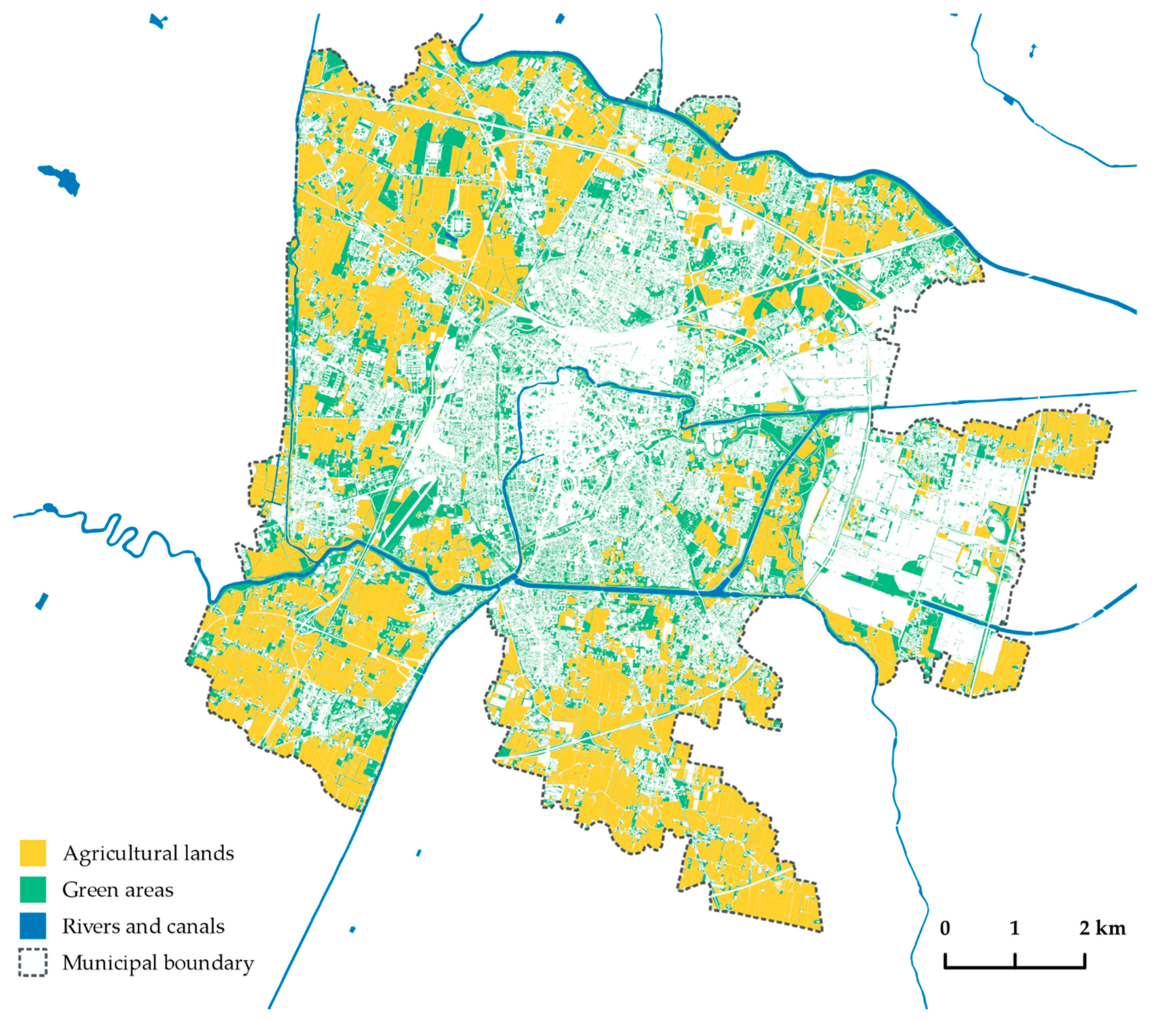
| Green Area Category | Area | Percentage of Total Green Areas |
|---|---|---|
| Total | 52.23 km2 | 100% |
| Rural | 28.80 km2 | 55.14% |
| Non-rural | 23.43 km2 | 44.86% |
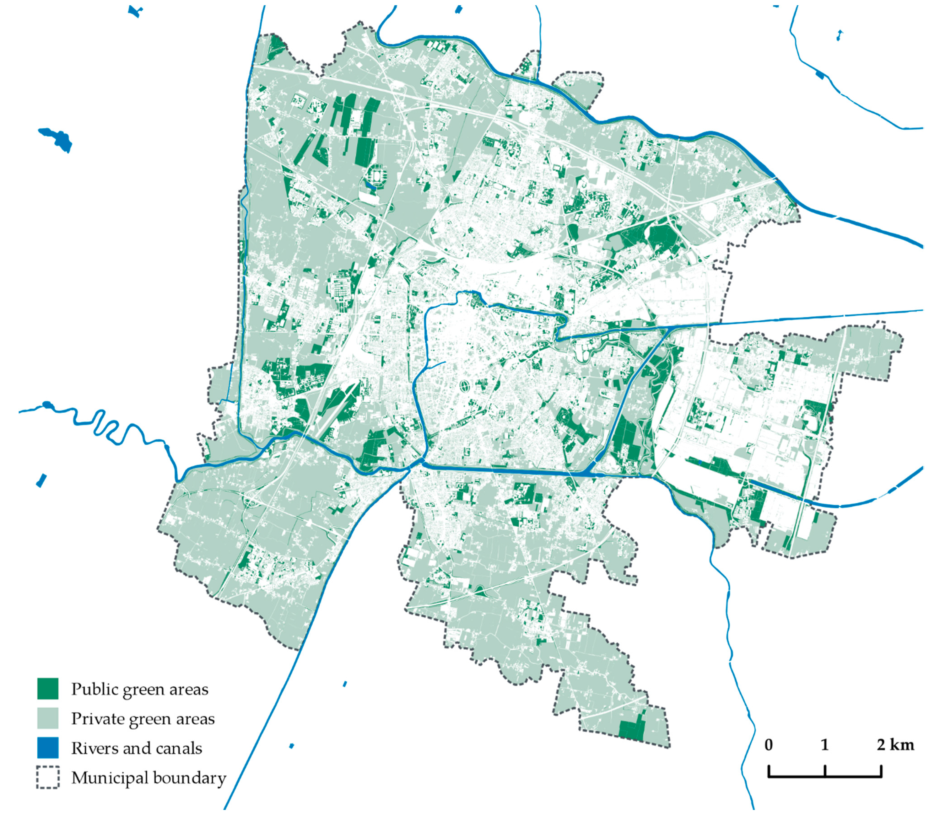
| Public | 10.25 km2 | 19.62% |
| Private | 41.98 km2 | 80.38% |
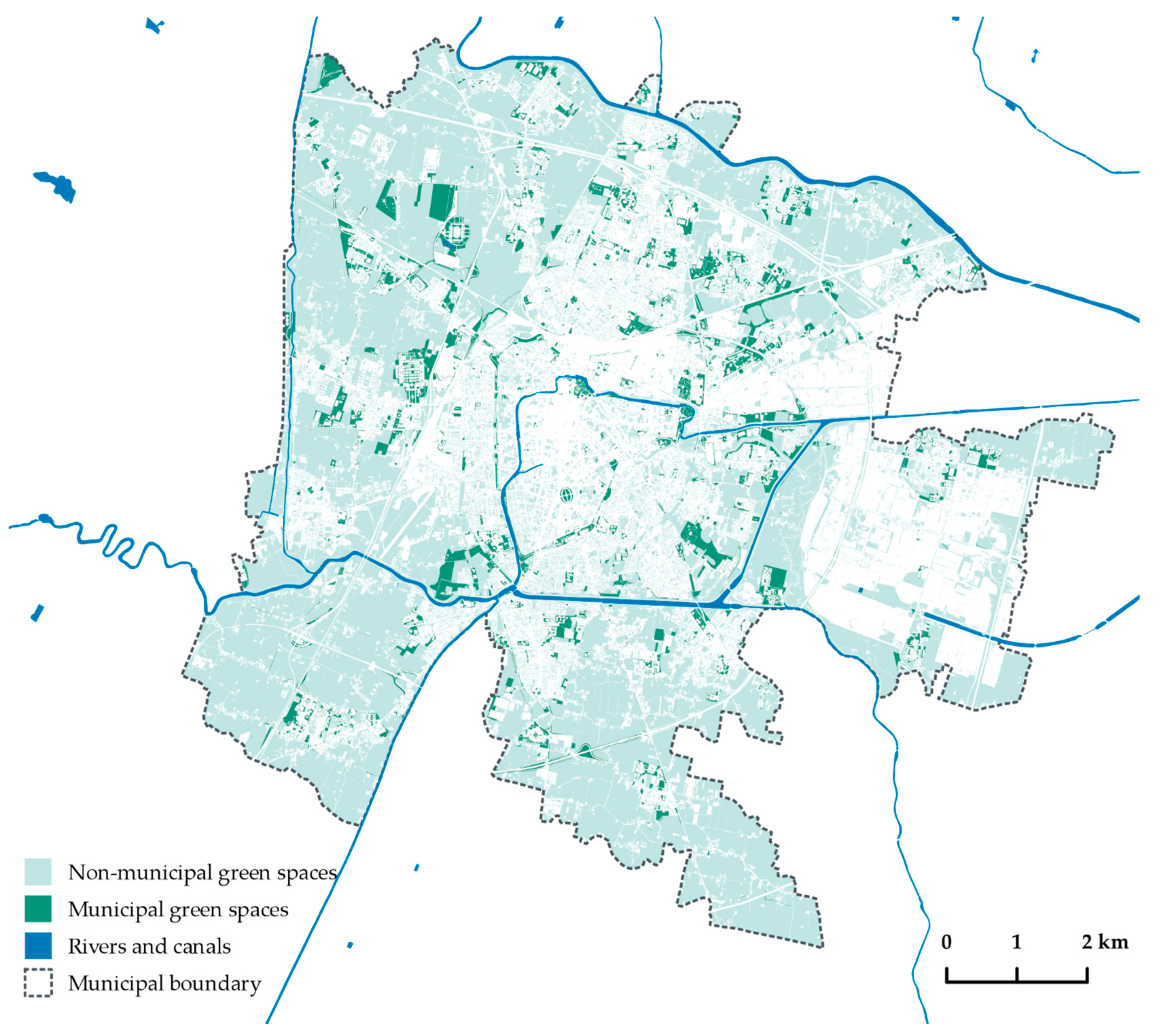
| Municipal | 5.02 km2 | 9.61% |
| Non-municipal | 47.21 km2 | 90.39% |
| Property | Total (km2) | Rural Green (km2) | Non-Rural Green (km2) | Percentage of Rural Green (%) | Percentage of Non-Rural Green (%) |
|---|---|---|---|---|---|
| Municipal UGS | 5.03 | 1.22 | 3.81 | 24.25 | 75.75 |
| Public, non-municipal UGS | 5.22 | 1.71 | 3.51 | 32.76 | 67.24 |
| Private UGS | 41.98 | 25.89 | 16.09 | 61.67 | 38.33 |
| Urban Unit Code | Urban Unit | Pop. | Area (km2) | Pop. Density per km2 | Total UGS (m2 PC) | Rural UGS (m2 PC) | Public UGS (m2 PC) | Private UGS (m2 PC) | Municipal UGS (m2 PC) |
|---|---|---|---|---|---|---|---|---|---|
| 1.1 | Piazze | 6893 | 0.80 | 8616.25 | 13.88 | 0.19 | 2.44 | 11.45 | 1.11 |
| 1.2 | Savonarola | 6560 | 1.19 | 5535.86 | 63.28 | 1.03 | 24.80 | 38.48 | 13.14 |
| 1.3 | Santo - Portello | 6975 | 1.63 | 4292.31 | 65.11 | 0.69 | 31.76 | 33.35 | 17.05 |
| 1.4 | Prato della Valle | 3272 | 0.76 | 4305.26 | 68.01 | 1.30 | 27.85 | 40.16 | 15.51 |
| 1.5 | Città Giardino | 4168 | 0.78 | 5371.13 | 64.86 | 2.99 | 16.63 | 48.22 | 12.89 |
| 2 | Sacra Famiglia | 7327 | 2.77 | 2640.36 | 231.83 | 83.74 | 90.61 | 141.22 | 38.14 |
| 3 | San Giuseppe | 7463 | 1.24 | 6023.41 | 40.76 | 0.30 | 6.24 | 34.52 | 3.83 |
| 4.1 | Porta Trento Sud | 2468 | 0.63 | 3936.20 | 59.34 | 0.00 | 6.02 | 53.32 | 4.77 |
| 4.2 | Porta Trento Nord | 625 | 0.46 | 1346.98 | 457.83 | 184.84 | 123.97 | 333.86 | 123.24 |
| 5.1 | Fiera | 2094 | 1.02 | 2061.02 | 96.86 | 13.77 | 46.31 | 50.55 | 43.55 |
| 5.2 | Stazione | 2274 | 0.83 | 2749.70 | 77.24 | 11.12 | 37.09 | 40.15 | 9.98 |
| 6 | Stanga | 3751 | 1.40 | 2671.65 | 117.39 | 19.13 | 58.08 | 59.31 | 48.55 |
| 7 | Forcellini | 9836 | 2.66 | 3697.74 | 132.63 | 31.70 | 41.30 | 91.33 | 23.10 |
| 8 | Madonna Pellegrina | 10964 | 2.23 | 4909.99 | 91.02 | 22.45 | 26.52 | 64.51 | 18.50 |
| 9 | Sant’Osvaldo | 6646 | 1.08 | 6148.01 | 68.36 | 10.77 | 9.75 | 58.61 | 7.03 |
| 10 | Voltabarozzo | 5272 | 2.07 | 2549.32 | 227.63 | 130.88 | 20.90 | 206.73 | 14.85 |
| 11 | SS. Crocefisso | 4612 | 2.44 | 1887.07 | 365.24 | 221.59 | 46.17 | 319.07 | 13.80 |
| 12 | Salboro | 2596 | 4.71 | 551.40 | 1503.08 | 1274.32 | 94.64 | 1408.44 | 32.94 |
| 13 | Guizza | 12770 | 4.25 | 3007.54 | 203.04 | 135.60 | 23.96 | 179.07 | 23.02 |
| 14 | Mandria | 10248 | 8.92 | 1149.27 | 662.69 | 461.45 | 48.45 | 614.24 | 25.39 |
| 15 | Brusegana | 7292 | 3.57 | 2041.43 | 319.30 | 176.99 | 95.66 | 223.75 | 6.49 |
| 16 | Cave | 4210 | 2.07 | 2030.87 | 255.52 | 126.39 | 75.43 | 180.09 | 72.55 |
| 17 | Brentelle | 4274 | 2.60 | 1645.11 | 425.47 | 236.57 | 45.74 | 379.84 | 25.76 |
| 18 | Sant’ignazio | 3791 | 1.37 | 2775.26 | 242.66 | 156.46 | 33.00 | 209.66 | 31.21 |
| 19 | Montà | 1196 | 0.91 | 1309.97 | 613.94 | 416.81 | 75.28 | 538.66 | 68.88 |
| 20 | Ponterotto | 2768 | 2.82 | 982.95 | 801.02 | 607.42 | 119.33 | 681.70 | 53.08 |
| 21 | Sacro Cuore | 4903 | 4.96 | 988.71 | 767.44 | 520.22 | 133.60 | 633.84 | 83.24 |
| 22 | Altichiero | 4111 | 3.54 | 1162.94 | 625.81 | 388.66 | 73.02 | 552.80 | 52.34 |
| 23 | Pontevigodarzere | 5302 | 1.91 | 2771.56 | 205.12 | 108.11 | 31.42 | 173.70 | 13.98 |
| 24 | San Carlo | 15,044 | 2.23 | 6761.35 | 53.69 | 10.29 | 16.75 | 36.94 | 15.11 |
| 25.1 | Arcella | 15,944 | 2.25 | 7092.53 | 40.99 | 2.56 | 8.71 | 32.28 | 7.60 |
| 25.2 | San Bellino | 3460 | 0.34 | 10267.06 | 31.79 | 0.30 | 3.18 | 28.61 | 2.74 |
| 26 | Mortise | 6503 | 1.89 | 3438.92 | 153.63 | 72.90 | 45.68 | 107.95 | 30.95 |
| 27 | Torre | 4496 | 3.07 | 1466.41 | 467.90 | 288.98 | 40.02 | 427.88 | 27.17 |
| 28 | San Lazzaro | 1838 | 3.44 | 534.61 | 669.18 | 270.77 | 311.46 | 357.72 | 108.09 |
| 29 | Ponte di Brenta | 3470 | 1.27 | 2727.99 | 150.88 | 21.23 | 17.74 | 133.14 | 13.22 |
| 30.1 | Zona Industriale | 575 | 8.07 | 71.29 | 4096.68 | 1464.42 | 1888.52 | 2208.17 | 55.48 |
| 30.2 | Terranegra | 242 | 1.18 | 205.61 | 3541.26 | 1941.74 | 1749.26 | 1792.00 | 472.61 |
| 31 | Camin | 4052 | 2.25 | 1800.09 | 377.63 | 261.16 | 44.56 | 333.07 | 31.92 |
| 32 | Granze | 877 | 1.73 | 505.77 | 1023.89 | 647.74 | 311.21 | 712.69 | 50.32 |
| PADUA | 211,162 | 93.31 | 2263.09 | 247.35 | 136.39 | 48.54 | 198.80 | 23.77 |
| Property | Strategies for Rural UGS | Strategies for Non-Rural UGS |
|---|---|---|
| Private | - Undertake initiatives to prevent the abandonment of crop fields and allow accessibility of their borders - Incentive peri-urban social farming, agroecology, and short chains to supply city consumers [69] | - Protect and incentive private vegetation development [27] - Consider the location and distribution of relevant private green spaces for environmentally centred plans and initiatives [31] |
| Public, non-municipal | - Foster connectivity and accessibility by pedestrian and cycle paths connected to urban GI - Encourage teaching and educational activities involving children and students [70] | - Promote public accessibility through agreements between Municipalities and other public institutions - Create and enhance urban GI leaning on existing city network systems |
| Municipal | - Promote their use as allotments or community gardens [71] - Consider the reuse of uncultivated fields as semi-natural peri-urban buffer zones connected to urban GI | - Increase accessibility to public uses with pocket parks or small public urban green spaces [72] - Promote trade-ins of land plots with other public or private actors to enhance green spaces continuity |
Publisher’s Note: MDPI stays neutral with regard to jurisdictional claims in published maps and institutional affiliations. |
© 2021 by the authors. Licensee MDPI, Basel, Switzerland. This article is an open access article distributed under the terms and conditions of the Creative Commons Attribution (CC BY) license (https://creativecommons.org/licenses/by/4.0/).
Share and Cite
Pristeri, G.; Peroni, F.; Pappalardo, S.E.; Codato, D.; Masi, A.; De Marchi, M. Whose Urban Green? Mapping and Classifying Public and Private Green Spaces in Padua for Spatial Planning Policies. ISPRS Int. J. Geo-Inf. 2021, 10, 538. https://doi.org/10.3390/ijgi10080538
Pristeri G, Peroni F, Pappalardo SE, Codato D, Masi A, De Marchi M. Whose Urban Green? Mapping and Classifying Public and Private Green Spaces in Padua for Spatial Planning Policies. ISPRS International Journal of Geo-Information. 2021; 10(8):538. https://doi.org/10.3390/ijgi10080538
Chicago/Turabian StylePristeri, Guglielmo, Francesca Peroni, Salvatore Eugenio Pappalardo, Daniele Codato, Antonio Masi, and Massimo De Marchi. 2021. "Whose Urban Green? Mapping and Classifying Public and Private Green Spaces in Padua for Spatial Planning Policies" ISPRS International Journal of Geo-Information 10, no. 8: 538. https://doi.org/10.3390/ijgi10080538
APA StylePristeri, G., Peroni, F., Pappalardo, S. E., Codato, D., Masi, A., & De Marchi, M. (2021). Whose Urban Green? Mapping and Classifying Public and Private Green Spaces in Padua for Spatial Planning Policies. ISPRS International Journal of Geo-Information, 10(8), 538. https://doi.org/10.3390/ijgi10080538