Abstract
Localization method based on skyline for visual geo-location is an important auxiliary localization method that does not use a satellite positioning system. Due to the computational complexity, existing panoramic skyline localization methods determine a small area using prior knowledge or auxiliary sensors. After correcting the camera orientation using inertial navigation sensors, a fine position is achieved via the skyline. In this paper, a new panoramic skyline localization method is proposed that involves the following. By clustering the sampling points in the location area and improving the existing retrieval method, the computing efficiency of the panoramic skyline localization is increased by fourfold. Furthermore, the camera orientation is estimated accurately from the terrain features in the image. Experimental results show that the proposed method achieves higher localization accuracy and requires less computation for a large area without the aid of external sensors.
1. Introduction
Visual geo-location is an important branch of computer vision [1,2,3]. By extracting visual features from images and comparing with the corresponding datasets, the position and the orientation (i.e., heading angle, pitch and roll) of the camera used can be obtained [4,5]. Skyline localization is an important visual geo-location method in the field environment, which is widely used for unmanned systems, e.g., unmanned vehicles [6,7]. Skyline localization can be categorized into local skyline localization and panoramic skyline localization according to the Field of View (FoV) of the retrieved images. Compared with local skyline localization, panoramic skyline localization has the following challenges. First, since the panoramic image contains the skyline with FoV of , there is a huge amount of data processing for feature extraction and calculation [8]. Second, the pitch of the camera has almost no effect on the local skyline, while the roll affects the rotation of the skyline. However, if the optical axis of the camera is not parallel to the horizontal plane, the acquired panoramic skyline will produce a sinusoidal distortion, which will affect the subsequent localization [9].
In this paper, a new panoramic skyline localization method is proposed, which achieves the panoramic skyline localization in a large area without using any auxiliary sensors (e.g., electronic compass, inertial navigation, accelerometer, etc.) and auxiliary information, e.g., from Geographical Information System (GIS). The novel contributions of this paper are as follows. First, a panoramic skyline coarse-localization method based on the skyline lapel points is introduced, including Digital Elevation Model (DEM) skyline clustering and matching method, for fast elimination of a large number of position candidate points. As far as we know, this is the first time that a DEM clustering is used for panoramic skyline localization. Second, a camera orientation estimation method based on the skyline lapel points is proposed. According to the difference between the lapel points in the image and DEM, the camera orientation at each candidate point is estimated for rapid confirmation of the skyline localization result.
2. Related Works
2.1. Panoramic Skyline Localization
There are a few panoramic skyline localization methods that are quite different due to their application in different scenarios. For example, in [10] a panoramic skyline localization method is used on Mars exploration vehicles, as illustrated in Figure 1. After capturing the panoramic image, the extracted skyline is calibrated by using the high-precision orientation sensor. This is to enable the skyline to be transformed into the horizontal state and then compared with a small range of DEM skylines. However, the accuracy of the commonly used sensors is relatively low, and the inertial navigation system produces cumulative errors when the system has run for a long time.
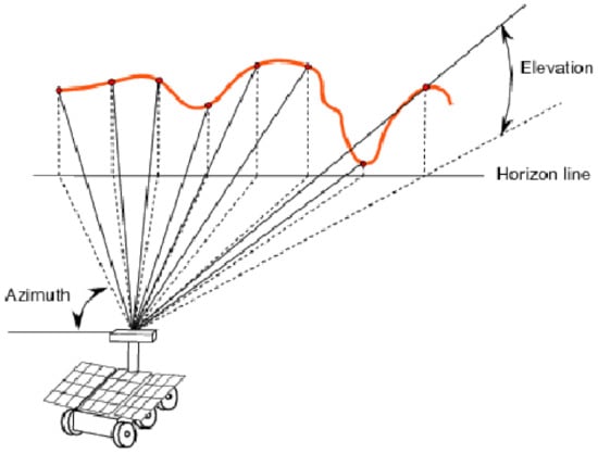
Figure 1.
The Mars rover takes photos and extracts the skyline.
In [9], the panoramic skyline localization is used for unmanned boats near an archipelago. The omni-directional camera on the unmanned boats is used to capture the image of the surrounding sea, extract the skyline and estimate the camera orientation. After the image skyline is corrected, it is compared with DEM skylines to determine the position of the unmanned boats as illustrated in Figure 2. A deep neural network is used to extract the waterline in the image, which is used to estimate the camera’s orientation. This method is ingenious, but cannot be used in land environment since there are no waterlines as reference.
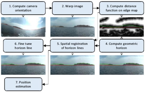
Figure 2.
Flowchart of skyline localization of unmanned boat [9]. It can be seen that due to the turbulence of the unmanned boat, the skyline of the original collected image has a large distortion. Through the second step of calibration, the distortion has been corrected.
In [11], the panoramic skyline localization is used in the urban area. Using a camera with fish-eye lens placed on the roof of a vehicle, the image skylines are extracted and compared with the rendering image generated by the 3-dimensional (3D) model of the city, so as to determine the location of the vehicle as illustrated in Figure 3. It is difficult to use this method in the field. First of all, it is difficult to use a fish-eye camera since many mountains are far away and therefore cannot be photographed. Secondly, for urban environment it is only necessary to process the dataset for the location of the sparse road network. Finally, since roads in urban area are relatively flat, the method does not need to deal with the distortion caused by the camera orientation, but only the distortion due to fish-eye lens.
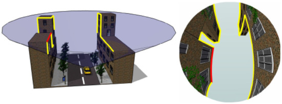
Figure 3.
Fish-eye camera takes urban images and extracts skyline.
2.2. Camera Orientation Estimation
In addition to camera orientation estimation and skyline correction in panoramic skyline localization (see Section 2.1), the camera orientation can also be estimated by local skyline localization. The method in [12] uses the first ridge line under the skyline as a reference to extract the contour words and compare them with the features in the dataset to determine its location. Since the contour words are sensitive to the camera orientation, this method also introduces the camera orientation estimation, referred as enumeration method, which is illustrated in Figure 4. Firstly, the ranges of the various parameters of the camera orientation are determined (e.g., FoV is [0, 70], roll is [−6, 6]). This is followed by using different parameter combinations to calculate the score of skyline matching. Where a certain parameter combination gets a high score in the correct heading angle, the combination of the parameters is considered as the real parameters of the camera. This method is simple and effective, but the computational time is high.
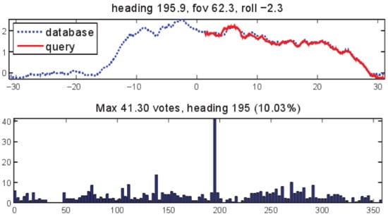
Figure 4.
Enumeration method for estimating camera orientation. Using a combination of various parameters within a predetermined range, the skyline with the highest matching score after calibration is found to determine the camera orientation.
The method in [13] uses the semantic information in images to estimate the camera pose as illustrated in Figure 5. Unlike the other skyline localization methods, the 3D model of this method adds corresponding semantic attributes through the GIS data of the region (i.e., the types and shapes of various regions are identified on the 3D model, including mountains, forests, glaciers, waters, etc.). The corresponding retrieved images also represent the various types of regions in the image by semantic segmentation. By calculating the coincidence of each region in the image with the corresponding region in the 3D model, the camera orientation is deduced. However, there are many limitations with this method. The GIS data of the area must be included, and the semantic information of the area should be relatively rich. Furthermore, under special weather conditions (e.g., haze), the semantic information of the image may disappear, so the method cannot be used.
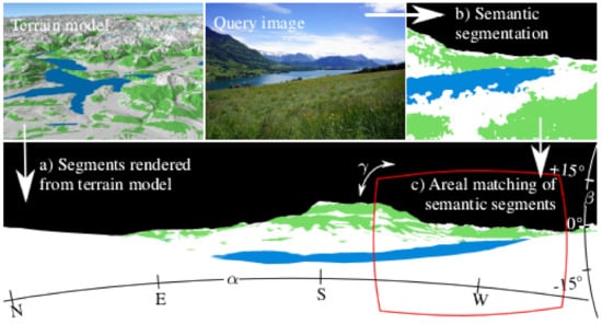
Figure 5.
Camera pose estimation based on semantic segmentation. Through semantic segmentation of the image, various geomorphic regions are identified, and the camera orientation is determined by matching with the terrain model containing GIS data.
There are also methods of determining skyline location by extracting features that are independent of rotation, so the estimation of camera orientation is unnecessary. In [14], the skyline is divided into several convex and concave curve segments as illustrated in Figure 6. These curve segments are rotated and normalized, and the area between the curve and the horizontal axis is encoded, so that the features are independent of camera parameters. This method has produced better effect in the desert area. However, it is more sensitive to noise, and any rotation will affect the end position of the skyline concave segment. Furthermore, the distortion of the panoramic skyline is more complex than that of the local skyline, which limits the application of this method in the panoramic skyline.
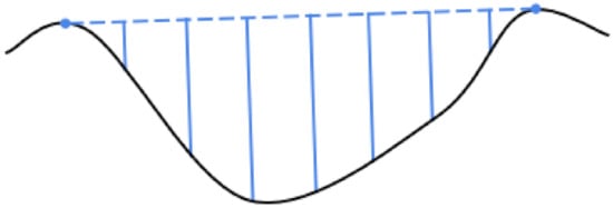
Figure 6.
Skyline features of concavity.
2.3. Clustering of Skyline Localization Datasets
The skyline clustering method aims to classify similar skylines and improve the retrieval efficiency, which is more important, and various researchers [12,14,15] regard it as one of the topics to be studied in the future. Zhu et al. [16] studied the skyline clustering of local skyline localization. Firstly, after obtaining dense and uniform skyline samples, the skyline dataset is divided into four sub regions (with yaw angle of , , and ), and the range of skyline in each sub interval is . Secondly, in each sub region, similar skylines are merged into the same region, referred as tolerance region, and only one skyline is reserved for each tolerance region. Although the effect is small in complex terrain, the sampling density is greatly reduced in the flat area as illustrated in Figure 7. This method cannot be applied to a panoramic skyline because the four directions of tolerance regions are completely different due to the terrain.
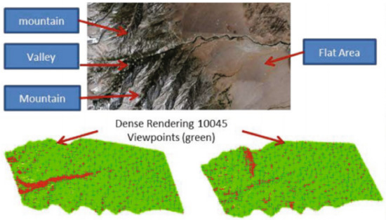
Figure 7.
The effect of clustering DEM skyline dataset. (Top): The terrain of the localization area; and (Bottom) results of clustering DEM skylines in and directions, respectively. The green points are the sampling points of the DEM skyline, and the red points are the tolerance regions. The sampling points of a skyline in two directions are different due to the influence of terrain.
3. Materials and Methods
Based on the previous work, this paper uses lapel points [17], the feature of the cross point between skyline and ridge line (as illustrated in Figure 8), to cluster the DEM skylines in order to accelerate the matching efficiency of panoramic skyline. Furthermore, a new camera orientation estimation method is proposed, which only depends on the image features and the corresponding features of DEM without using external sensors to estimate the camera orientation. Figure 9 outlines the various processes of the proposed method.
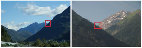
Figure 8.
The lapel point of a skyline: (left) left lapel point of skyline; and (right) right lapel point of skyline.
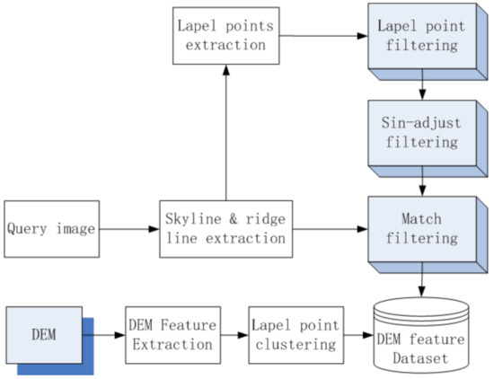
Figure 9.
The flow chart of the proposed method.
3.1. Clustering of the DEM Lapel Points
In the complex terrain environment, the skyline changes significantly over a short distance [16] as illustrated in Figure 10. Thus, the dense sampling is the premise to ensure the accuracy of skyline positioning, but the more intensive skyline sampling will lead to the decrease of retrieval efficiency in skyline localization.

Figure 10.
The intense change of the skyline in a mountainous area. Although View1 and View2 are only 30 m apart, the skyline along the same direction changes greatly due to the promixity of the mountains.
The proposed clustering method uses the lapel points to cluster DEM skylines, so as to merge similar DEM skylines in close proximity. Compared with the method in [16], the proposed method does not divide the dataset by angle in order to satisfy the needs of panoramic skyline localization. In addition, a coarse localization of skyline algorithm is designed through the lapel point matching, which is to reduce the required computation in matching high-density skyline and improve the retrieval efficiency of skyline. The process of clustering DEM lapel points is outlined in Figure 11.
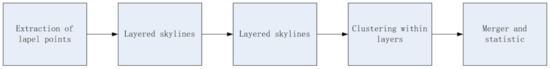
Figure 11.
The flow chart of clustering lapel points.
Firstly, after extracting the lapel points of each skyline, the dataset is stratified according to the number of lapel points, where the number of lapel points in each layer is the same. Secondly, according to the sequence and spatial distance of lapel points, the clustering method is used to group the lapel points of each layer. Finally, the clustering results of each layer are merged to generate the cluster of lapel points in the region, and the statistical features of various types are extracted.
3.1.1. Extraction of DEM Lapel Points
By calculating the first derivative of the depth value of each point on the DEM skyline [17], we obtain the lapel points of the DEM skylines. The format of each DEM skyline point is shown in Table 1.

Table 1.
DEM lapel points information list.
Starting from the North, the features of lapel points for each DEM skyline are saved successively. Type is the type of lapel point, which is of two types: left and right. Angle is the angle of the lapel point relative to North with value range [0, 360]. Angle is the angle between the current lapel point and the next adjacent lapel point in the clockwise direction with value range [0, 360] (see Figure 12). (L-distance, R-distance) refers to the depth of the skyline on the left and right sides of the corresponding lapel point, as illustrated in Figure 13.
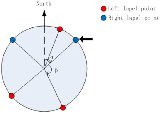
Figure 12.
The angle between the North of the lapel point and the adjacent point in the clockwise direction. The current selected lapel point is the right lapel point indicated by the black arrow, and its Angle is , and the Angle is .
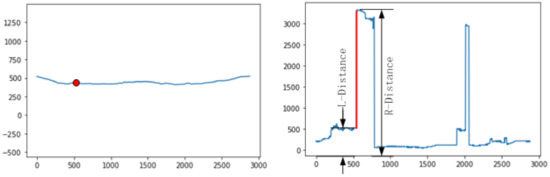
Figure 13.
(L-distance, R-distance) of lapel point: (left) DEM skyline with the position of a lapel point denoted by a red dot; and (right) the depth of the skyline in (left), where the red line denotes the difference in depth in (left), and the L-distance and R-distance are denoted by black arrows, representing the depth of left and right sides of lapel point, respectively.
3.1.2. Layering of the DEM Lapel Points
After extracting the lapel points of each skyline in DEM, the number of the lapel points is saved in a 2-dimension matrix (as shown in Figure 14).
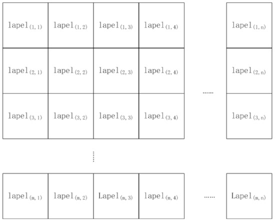
Figure 14.
The lapel point matrix of the dataset. The size of the matrix is related to the DEM area and skyline sampling density. The element in the matrix represents the number of lapel points on the skyline .
According to the number of lapel points, the dataset can generate a heatmap of the sampling points as shown in Figure 15. It can be seen that when the sampling distance is large, the number of lapel points changes greatly. Conversely, when the sampling distance is small, the change of lapel point number is relatively small.
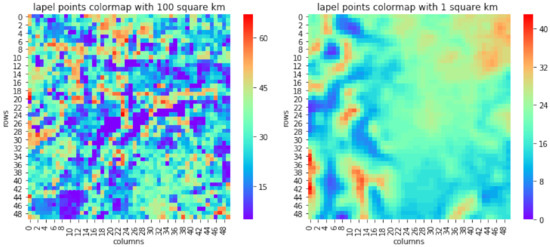
Figure 15.
The heatmap of the lapel points. The size of the heatmap is related to the DEM area and the skyline sampling density. The dot in the heatmap represents the number of lapel points of the skyline in row i and column j.
The dataset is divided into several layers according to the number of lapel points in the region as illustrated in Figure 16. The specific method is
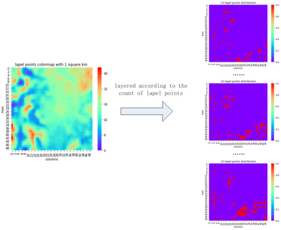
Figure 16.
The layering heatmap according to the number of each lapel point.
After layering, the number of the lapel points in each layer is the same.
3.1.3. Clustering of the DEM Skylines
After dividing the dataset into different layers, each layer has the same number of lapel points. However, the skyline with the same number of lapel points does not represent the same attributes. This is because some points are relatively far away from other points, while some points are closer, and the type of lapel points may differ.
The purpose of skyline clustering is to classify the skylines with the closer distance and the same lapel point sequence into the same category, so as to improve the efficiency of skyline retrieval. The steps of the clustering are as follows. Firstly, code the lapel points of a skyline from the North and save the types of each lapel point in turn to form a lapel point sequence “l-r-r-l-l-r-r” as observed from a point A as illustrated in Figure 17(left). Secondly, determine the lapel point sequences that are the same in the loop. This is needed because the observed lapel points near North will change the lapel point sequence due to A being slightly moved. For example, the lapel point sequence observed from A in Figure 17(right) is “r-l-r-r-l-l-r”. Since the two lapel sequences are very close in distance, the skyline with the same cycle of lapel points is considered the same. Finally, cluster the skylines with the lapel point sequences. Since the number of clusters cannot be specified in advance, Density-Based Spatial Clustering of Applications with Noise (DBSCAN) algorithm is used for clustering. Unlike the partition and hierarchical clustering methods, DBSCAN defines a cluster as the largest set of densely connected points. It divides the region with sufficiently high density into clusters (as illustrated in Figure 18) and finds clusters of arbitrary shape in a noisy spatial database [18].
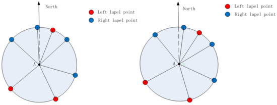
Figure 17.
The influence of the position of an observation point on the sequence of lapel points: (left) Point A is the current observation point; and (right) the lapel point sequence as observed from a slightly moved A. The dotted circle represents the original position of A.
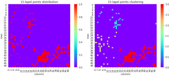
Figure 18.
The clustering of the lapel point sequence: (left) Distribution of skyline with group of 8 lapel points; and (right) the result of the clustering by lapel point sequence and distance. It can be seen that the skyline with lapel number 8 is divided into three categories.
After clustering, the skyline with the same number of lapel points is divided into different categories according to distance and type of lapel points. In the same category, the features of skyline lapel points have certain similarities, as illustrated in Figure 19.
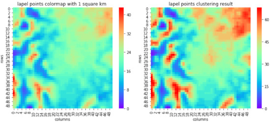
Figure 19.
A cluster of lapel points: (left) The heatmap of lapel points within 1 km. The color of each point denotes the corresponding number of lapel points; and (right) the clustering result of (left). The color of each point denotes the corresponding category of lapel points.
3.1.4. Listing the DEM Lapel Points
The DEM skylines are classified and managed according to the lapel point, and each type of skyline has similar lapel point feature. By saving each type of skyline and creating an index table, the efficiency of the skyline retrieval is improved. The lapel point index table of skylines is a linked list, where each node stores the type and angle features of the skyline lapel point. The node contents of the index of a skyline are shown in Table 2. The angle features of a lapel point refer to the minimum and maximum value of Angle of the same index of the lapel point in the same skyline. It shows the range of lapel point angle of uniform index number in the same type of skyline.
Table 2.
Node contents of the index.
The index saves the type and angle of each lapel point in turn. Figure 20 illustrates how the index of lapel points is determined.
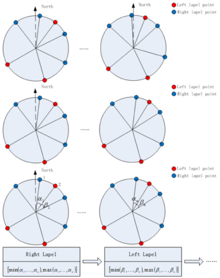
Figure 20.
The feature extraction map of skyline type lapels: (First row) n skylines in the same category considered by the clustering method to have the same geometry; (Second row) based on the lapel point sequence of the first skyline in the same category, adjust the sequence of the remaining skyline lapel points to correct the changes caused by the position of observation points; (Third row) statistics of the type and angle of each lapel point; and (Fourth row) skyline lapel point index, which records the type and angle range of each lapel point category.
3.2. Extraction of Image Skyline and Lapel Points
The skylines and ridge lines are extracted from the image using methods of semantic segmentation, such as U-Net [19]. The classification of lapel point type depends on the spatial relationship between the skyline and the ridge line. Compared with the ridge line matching proposed by other scholars, the lapel point reduces the accuracy requirement of ridge line extraction [17]. It only needs to extract the ridge line near the intersection point of ridge line and skyline. The effect of the extraction of lapel points of skyline is illustrated in Figure 21.

Figure 21.
The effect of the extraction skyline and lapel points. Red curve denotes the skyline and the ridge lines, where the top red curve is the skyline, and a blue square denotes a lapel point after manual verification and the ambiguous or incorrect lapel points are removed.
3.3. Panoramic Skyline Matching
Due to the large amount of data, existing methods only locate the panoramic skylines in a small area (less than 1 km) in order to improve the retrieval efficiency, and use sensor (e.g., as in [10]) or other special features as in [9] to obtain the camera orientation. In this paper, a clustering method based on lapel points is first proposed, and a lapel point matching algorithm is designed to improve the efficiency of skyline retrieval. Second, a camera orientation estimation method based on lapel points difference is proposed. The retrieval process of a panoramic skyline is outlined in Figure 22.
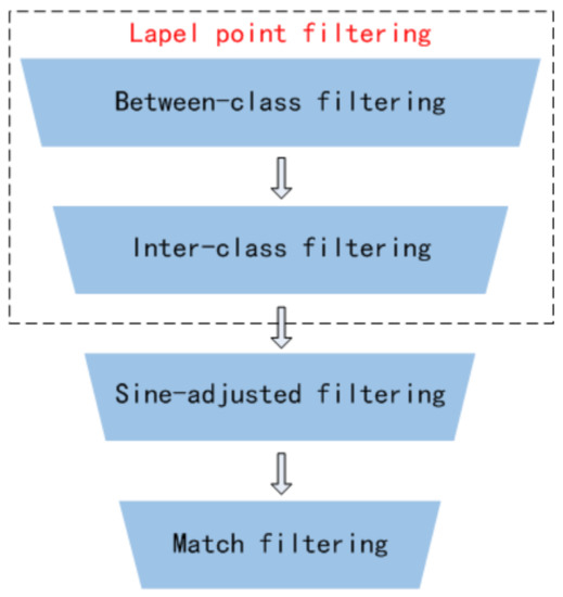
Figure 22.
The panoramic skyline retrieval process. The retrieval consists of four steps, with each step filtering out some candidate points, and the last step sorting them according to the matching results.
3.3.1. Between-Class Filtering
Between-class filtering refers to using the type and location of lapel points marked in the image to filter out candidate points that do not match completely in DEM skylines dataset. The filtering determines whether the remaining lapel points are within the angle range of corresponding type of lapel point after the first lapel point of an image is aligned with the same type of DEM. If all the image skyline lapel points are in the range of lapel points of the class, then the matching between classes is successful. Conversely, all skylines in the class are filtered out if they cannot match the lapel points of the image skyline.
Coarse matching is used to compare lapel points as illustrated in Figure 23. The skylines that do not match the lapel points are filtered out, and the number of skylines with the lapel points and the corresponding heading angles are recorded.
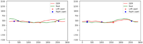
Figure 23.
Coarse matching: (Left) the state before the DEM skyline is coarsely matched with the image skyline; and (Right) the state after coarse matching between DEM skyline and image skyline. Through the coarse matching, the candidate yaw in the image can be determined at the same time.
When judging the match between the image skyline lapel points and DEM skyline lapel point category, a traversal method is used to align the first lapel point of the image skyline with the same type of lapel points in DEM category in clockwise direction. This is followed by checking the remaining skyline lapel points, including type matching and whether the position of image skyline lapel point is within the threshold of DEM skyline lapel point.
In the matching process, due to the self-similarity of terrain and the lack of lapel points in the image skyline, there may be multiple possible yaw candidates for the same DEM skylines as illustrated in Figure 24. This diversity gradually decreases with the completeness of the number of skyline lapel points.
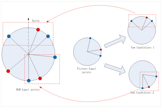
Figure 24.
For the same DEM skyline (enclosed in larger dotted red rectangles), the coarse matching of the image skyline may have multiple yaw candidates (enclosed in the smaller dotted red rectangles).
3.3.2. Intra-Class Filtering
Intra-class filtering removes the skyline with a large difference in lapel points among the selected lapel points categories, so as to reduce the number of candidate skylines for fine localization. It is similar to between-class filtering, but changes to , where the threshold is set to to limit width of the filter window. Between-class filtering and intra class retrieval improve the efficiency of skyline retrieval significantly, even though they are additional processing steps than direct retrieval. Suppose that the number of cluster points is n, and the number of skyline lines of each cluster is . Let the mean value of the number of skyline lines of lapel type be
The time complexity of the algorithm is given by , where is the number of classes considered by the algorithm. The time complexity of traversal is , where , thus, the efficiency of between-class filtering and intra class filtering are higher. However, the lapel point matching only eliminates the skyline through the lapel points, and the skyline with lapel points does not represent the same trend of skyline.
3.3.3. Orientation Estimation and Filtering
When the optical axis is not parallel to the horizontal plane (i.e., the pitch or roll of the camera is not ), the camera can produce a panoramic picture with a sinusoidal distortion (as illustrated in Figure 25).
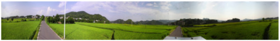
Figure 25.
Camera orientation causes sinusoidal distortion in the image. For a sloping path, the two sides of the picture are uplifted, whereas the middle part sinks to the right.
Similar distortions are also found in other studies as illustrated in Figure 26. Although choosing a suitable location on the land can avoid the large tilt, it is difficult to ensure that the platform is completely horizontal. Since no waterline is considered in [9], this paper proposes a new camera orientation estimation method, which only relies on the lapel points in the image to determine the candidate camera’s orientation and verifies the orientation according to the match with the skyline.
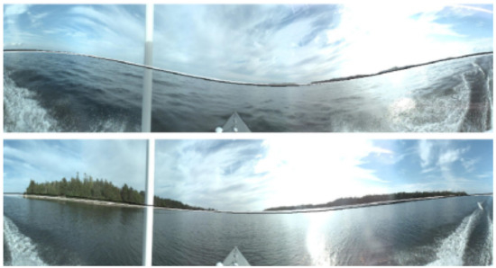
Figure 26.
Panoramic view from an unmanned aerial vehicle [3]. Due to the influence of sea waves, the images have a sinusoidal distortion.
The model of sinusoidal distortion at frequency caused by camera orientation is
where the parameters A and are defined in the bottom right of Figure 27. Since the height of DEM skyline dataset is the height from the camera of experimental vehicle to the ground, and h is 0 under normal conditions. The panoramic skyline contains only one period of sinusoidal distortion, so is also a fixed value. Therefore, three or more points on the sine curve can be identified, and the curve can be fitted by the least square method [20]. The whole fitting process is illustrated in Figure 27.
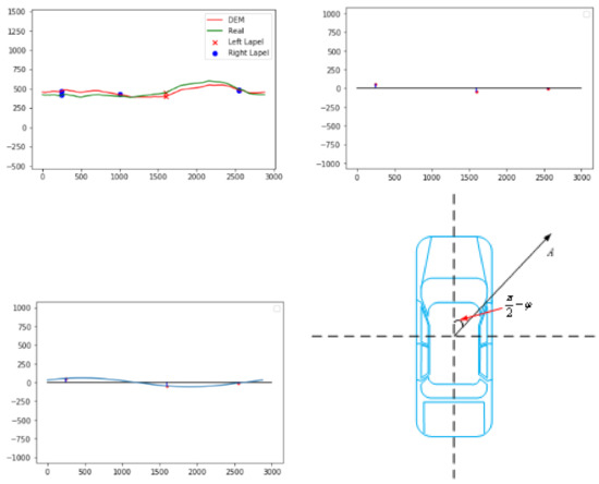
Figure 27.
The camera orientation estimation process: (Top-Left) Find the DEM skyline lapel points matching the image lapel points (i.e., the result of coarse positioning outlined in Section 3.3.2); (Top-Right) calculate the difference of lapel height; (Bottom-Left) fit the sine curve; and (Bottom-Right) the physical meaning of sine function curve parameters. The variable A represents the size of the superposition of roll and pitch vector in camera orientation, and represents the direction of the superposition.
The lapel height difference is
where is the height of the ith lapel point in DEM and is the height of the jth lapel point. This pair of lapel points is the result of the coarse filtering.
Through orthogonal decomposition, the vehicle orientation is obtained by fitting as follows. If the length of DEM skyline is , through the A and based on the sine curve fitting, the estimated pitch and roll are
and
When the parameter h fitted by the lapel height difference is not 0 and exceeds the preset threshold, then the DEM skyline does not match the image skyline and is marked as “the skyline difference is large”, so as to avoid the subsequent fine matching and improve the retrieval efficiency. The anomaly of parameter h is the necessary condition of skyline mismatching. For some mismatched skyline pairs, the sine function fitted by lapel points difference is also less than the threshold value (see Figure 28), which needs to be further filtered by skyline similarity calculation like the method in Section 3.3.4.
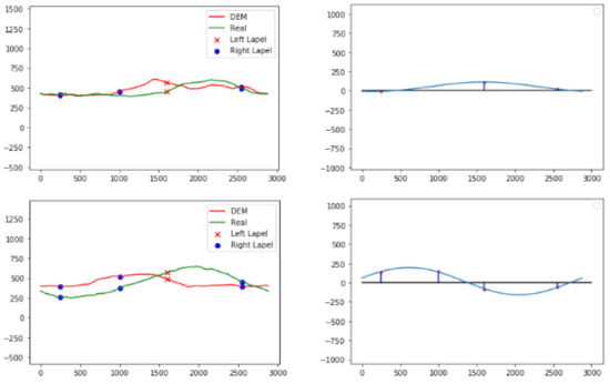
Figure 28.
The sine fitting results of mismatched skyline pairs: (Top row) h is large and the entire sine function shifts upward; and (Bottom row) the vertical offset of sine function is normal.
3.3.4. Skyline Calibration and Computing Similarity
Skyline calibration is used to determine the tilt of the camera’s platform (i.e., the magnitude and position of the tilt) to reverse compensate the image skyline, so that the image skyline is restored to the camera horizontal condition so as to obtain the true shape of DEM skyline. The restoration is using
where is the height of column i of the skyline and is the length of the skyline. The restoration method determines the offset caused by fitting sine wave at different positions of the skyline and compensates the skyline by the offset at the same position, so as to realize the image skyline calibration as illustrated in Figure 29 and Figure 30.
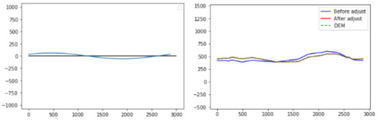
Figure 29.
Calibration effect of sinusoidal distortion: (Left) The sine curve as fitted in Section 3.3.3; and (Right) The effect of calibration. It can be seen that there is a significant difference between the DEM skyline and image skyline before and after calibration.
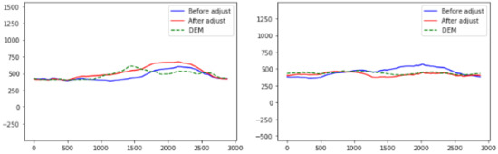
Figure 30.
An example of matching failure after sine correction. The features of skyline and DEM are matched in the two maps, but after correction, the difference of skyline pairs is significant, indicating that the locations of DEM sampling points for comparison are not the locations of where the images were taken.
Since the orientation of a skyline can be estimated from lapel points, the proposed method adopts the method similar to [10] and uses the square error (defined later) to determine the similarity. Since there may be more than one group of camera orientation estimated by lapel points, it is necessary to compute the similarity between the image skylines and the DEM skylines of each candidate parameter and select the minimum among the results. Since the lapel points pair is not completely aligned, the lapel point with the furthest distance is selected as the anchor point for the alignment of the two skylines, i.e.,
where and , respectively, represent the left and the right of the distances of lapel point j. Suppose an image skyline has n orientation candidates on a certain DEM skyline, and each candidate orientation is
where is ith candidate’s yaw, and and are sine correction parameters. The square error of each orientation is
The similarity of image skyline on a DEM skyline is the minimum of all candidate pose similarity sets on the DEM skyline, i.e.,
4. Results and Discussion
4.1. Experimental Site and Equipment
The experimental site is located in the suburb of Changsha, China, as shown in Figure 31. The experimental area is about (28.08 N, 112.69 E∼28.15 N, 112.76 E), which is a hilly area with few human-made buildings.
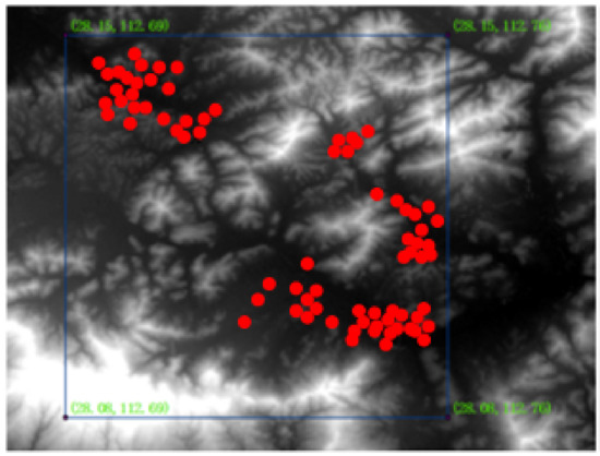
Figure 31.
The DEM data of experimental area. The red dots in the figure represent the place where the pictures were taken in the experiments.
The DEM data spatial resolution used in the experiment is 10 m. After a 3D terrain model is constructed by OpenGL, the rendered DEM skyline image is generated by a virtual camera. The resolution of the rendered image is , and the horizontal FoV and vertical FoV are and , respectively, (as shown in Figure 32).
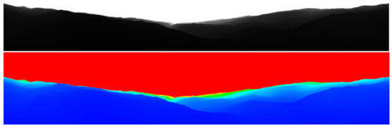
Figure 32.
Rendering of DEM skyline generated by 3D model: (Top) Rendering of skyline generated from DEM data at selected sampling points, where the white area is the sky, the non-white area is the peak, and the gray scale represents the distance between the mountain and the observation point; (Bottom) pseudo-color map of (Top) to facilitate the viewing of details of the peak.
For the acquisition of the panoramic images, we used a camera with horizontal rotation controlled by command to rotate at a constant speed, which is fixed on the top of the experimental vehicle and has a lifting lever. When the camera is raised, the height from the ground is about 3.3 m (as shown in Figure 33).
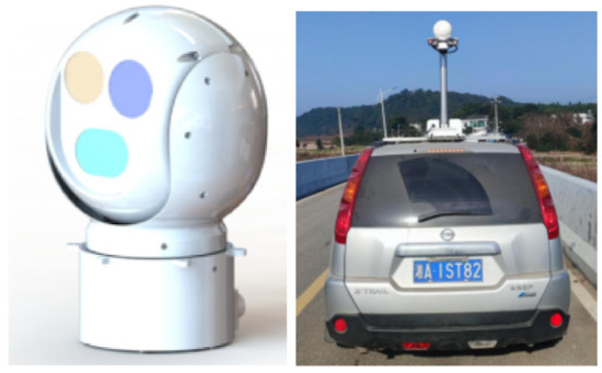
Figure 33.
Equipment used in the experiment: (Left) Camera can be rotated and images are captured by command; and (Right) installation of the camera on the experimental vehicle.
During the image capture, the lifting lever raises the camera and captures images from different heading angles in turn (see Figure 34). Using an image stitch algorithm, the images are combined as a panoramic image as shown in Figure 35.
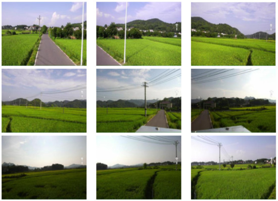
Figure 34.
Images captured by the experimental vehicle. The FoV of the camera is and each image was captured every rotation of the camera. The resolution of each image is . It can be seen that there are some overlaps between the adjacent images.
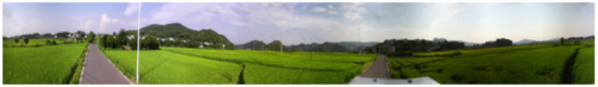
Figure 35.
The panoramic image. Using the image stitch algorithm, the sub images in Figure 34 are merged into a panorama. The left side is the image captured when the optical axis of the camera coincides with the central axis of the vehicle.
During the image capture, GPS and inertial navigation were used to record the position and camera orientation (as shown in Table 3).
Table 3.
The orientation of the image in Figure 35.
A total of 96 groups of images were captured, and the location and orientation were recorded. In order to avoid the influence of foreground occlusion on localization, the locations were selected to be far away from a mountain peak, and where the foreground interference is less.
All the experiments were run on a laptop, the CPU of which was Intel(R) Core(TM) i5-7200U @ 2.50 GHz (4 CPUs) and with a size of RAM is 16 G.
4.2. Camera Orientation Estimation
The orientation of the camera is determined in the case of successful localization of the restored skyline. The errors in the pitch and roll are determined as follows:
The estimated camera orientation is very close to the parameters of a vehicle inertial navigation system, as shown in Figure 36.
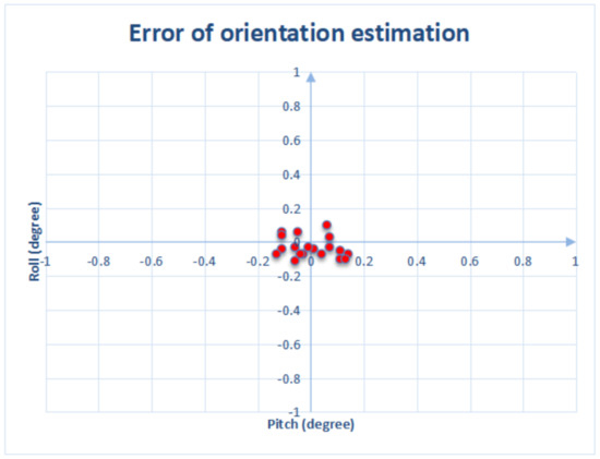
Figure 36.
Orientation estimation error. It can be seen that the estimated orientation is very close to the inertial navigation system.
Although the method estimates the camera orientation (i.e., yaw, roll and pitch) by comparing and fitting the lapel points, unlike the waterline method in [9], the matching and fitting of lapel points may have ideal results at the real point and its vicinity, thus reducing the localization accuracy. Thus, experiments were carried out to evaluate the proposed method, where the localization accuracy and efficiency are compared between estimating camera orientation and providing camera orientation. The experimental results show that the accuracy and efficiency of localization are improved by providing camera orientation as shown in Figure 37.
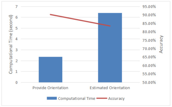
Figure 37.
The effects of positioning accuracy and efficiency between estimating orientation and providing orientation.
Furthermore, compared with the enumeration method in [12], the efficiency of our method is much higher, as shown in Figure 38.
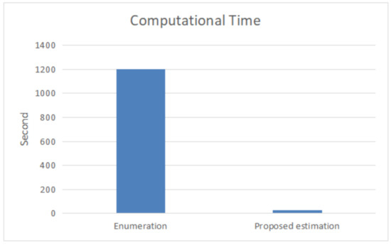
Figure 38.
Comparing the efficiency of the proposed orientation estimation method with the enumeration method in [12]. The range of roll and pitch of the enumeration method are both [−5, 5], step size is 0.1, and yaw step size is 1.
4.3. Camera Localization
In the experiment, the 96 groups of images were used, and the localization accuracy was determined. Experiments show that the accuracy of the proposed method is similar to that of directly using the traversal method, as shown in Figure 39.
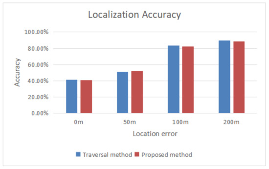
Figure 39.
The localization accuracy of the proposed method is similar to that of the traversal method.
A comparative experiment was also conducted on lapel point clustering, which improves the retrieval efficiency. Compared with traversing the lapel points, the retrieval efficiency of the cluster is improved by more than fourfold (see Figure 40).
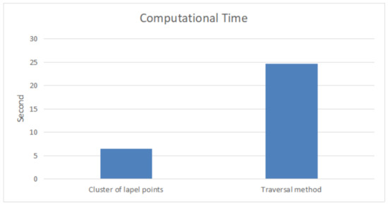
Figure 40.
Comparing lapel point clustering efficiency with traversal method.
The influence of the number of lapel points on retrieval efficiency is compared in Figure 41. It can be seen that reducing the number of lapel points in the image skyline decreases the retrieval efficiency. When the number of lapel points is reduced to one, the effect of lapel clustering almost disappears, and the speed of the algorithm is slightly slower than the traversal retrieval method.
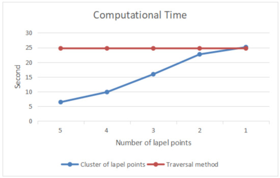
Figure 41.
The effect of the number of lapel points on the retrieval efficiency. If the lapel points in the skyline are removed, then the retrieval efficiency is greatly reduced.
4.4. The Influence of Lapel Point Error
The proposed clustering method using lapel points has greatly improved the localization efficiency, but the accuracy of lapel points also affects the accuracy of localization. Thus, two groups of experiments were designed to evaluate the influence of lapel points error on localization accuracy.
4.4.1. Influence of Adjacency Angle Error
Adjacency angle refers to the angle between adjacent lapel points in clockwise direction and indicates the distance between adjacent lapels. In the experiment, random noise was added to the adjacent angles of all lapel points on the skyline, and the change in localization accuracy was determined.
Denote the number of lapel points of a skyline as n, then
Denote the noise as and the random noise added to the adjacent angle of each lapel point as , then the adjacency angle of each lapel point is
By adding noise to the adjacency angle of lapel points and observing the change in localization accuracy, it can be seen that with the increase in noise, the accuracy of localization gradually decreases. When the noise is greater than , the downward trend is more obvious as shown in Figure 42.
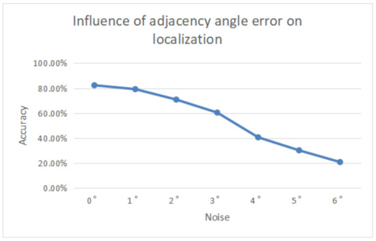
Figure 42.
The influence of adjacent angle noise on localization accuracy.
4.4.2. The Influence of Incorrect Lapel Points on Positioning
An incorrect lapel point refers to the error in the process of extracting the image skyline lapel points, including the lapel point type error caused by manual marking and the pseudo lapel point due to foreground obstacles. Experiment shows that these two types of errors are detrimental to localization, and incorrect lapel points result in localization failure.
The first experiment randomly selected a skyline lapel point in each image skyline, modified its type and counted the change of localization accuracy. The result is all the localization failed (as shown in Figure 43(left)). Furthermore, the second experiment randomly added a lapel point to each skyline, modified the relative information (adjacency angle, etc.) of the skyline lapel point, and determined the change in localization accuracy. The same results were obtained and shown in Figure 43(right).
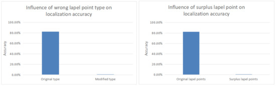
Figure 43.
The influence of incorrect lapel points: (Left) Influence of incorrect lapel point type on localization accuracy; and (Right) influence of surplus lapel points on localization accuracy.
5. Conclusions
In this paper, a new panoramic skyline location method is proposed. The DEM skylines are clustered according to the lapel points, and the retrieval algorithm of coarse positioning is proposed. A new camera orientation estimation method is also proposed. Without the aid of external sensors and according to the lapel points, the camera orientation is estimated, and the image skyline is verified. Experiments show that the proposed method has good performance in efficiency and accuracy.
In the future, lapel points will be added between ridge lines to extend the DEM multiple lapel points dataset. This is to complete the panoramic skyline localization method under multi-visibility environment, and minimize the localization effect of the algorithm in extreme environments such as rain, snow and haze. Furthermore, when some errors in the extraction of the image lapel points are encountered, they can be used to give the probability of lapel points similarity. Therefore, it is necessary to improve the robustness of the proposed methods. Finally, the refinement of image skylines and ridge lines is also worthwhile research, where the recognition of pseudo skylines and pseudo ridge lines caused by foreground obstacles (e.g., trees, artificial objects, etc.) can be utilized to improve the accuracy of skyline lapel point recognition, reduce manual intervention and improve the adaptability of the proposed method.
Author Contributions
Jin Tang and Fan Guo contributed to the conception of the study; Zhibin Pan performed the experiment; Zhibin Pan and Jin Tang contributed significantly to the analysis and manuscript preparation; Zhibin Pan, Jin Tang, and Tardi Tjahjadi performed the data analyses and wrote the manuscript; Zhibin Pan and Jin Tang helped perform the analysis with constructive discussions. All authors have read and agreed to the published version of the manuscript.
Funding
This research received no external funding.
Data Availability Statement
The data used to support the findings of this study are available from the corresponding author upon request.
Conflicts of Interest
The authors declare no conflict of interest.
References
- Brejcha, J.; Čadík, M. State-of-the-art in visual geo-localization. Pattern Anal. Appl. 2017, 20, 613–637. [Google Scholar] [CrossRef]
- Xin, X.; Jiang, J.; Zou, Y. A review of Visual-Based Localization. In Proceedings of the 2019 International Conference on Robotics, Intelligent Control and Artificial Intelligence, Shanghai, China, 20–22 September 2019; pp. 94–105. [Google Scholar]
- Piasco, N.; Sidibé, D.; Demonceaux, C.; Gouet-Brunet, V. A survey on visual-based localization: On the benefit of heterogeneous data. Pattern Recognit. 2018, 74, 90–109. [Google Scholar] [CrossRef]
- Baatz, G.; Saurer, O.; Köser, K.; Pollefeys, M. Large scale visual geo-localization of images in mountainous terrain. In Proceedings of the European Conference on Computer Vision, Florence, Italy, 7–13 October 2012; pp. 517–530. [Google Scholar]
- Dumble, S.J.; Gibbens, P.W. Efficient terrain-aided visual horizon based attitude estimation and localization. J. Intell. Robot. Syst. 2015, 78, 205–221. [Google Scholar] [CrossRef]
- Gupta, V.; Brennan, S. Terrain-based vehicle orientation estimation combining vision and inertial measurements. J. Intell. Robot. Syst. 2008, 25, 181–202. [Google Scholar] [CrossRef]
- Woo, J.; Son, K.; Li, T.; Kim, G.S.; Kweon, I.S. Vision-based UAV Navigation in Mountain Area. In Proceedings of the Iapr Conference on Machine Vision Applications, Tokyo, Japan, 16–18 May 2007; pp. 517–530. [Google Scholar]
- Fukuda, S.; Nakatani, S.; Nishiyama, M.; Iwai, Y. Geo-localization using Ridgeline Features Extracted from360 to degree Images of Sand Dunes. In Proceedings of the 15th International Conference on Computer Vision Theory and Applications, Valletta, Malta, 27–29 February 2020; pp. 621–627. [Google Scholar]
- Grelsson, B.; Robinson, A.; Felsberg, M.; Khan, F.S. GPS-level accurate camera localization with HorizonNet. J. Field Robot. 2020, 37, 951–971. [Google Scholar] [CrossRef]
- Chiodini, S.; Pertile, M.; Debei, S.; Bramante, L.; Ferrentino, E.; Villa, A.G.; Barrera, M. Mars rovers localization by matching local horizon to surface digital elevation models. In Proceedings of the 15th International Conference on Computer Vision Theory and Applications, Nagoya, Japan, 8–12 May 2017; pp. 374–379. [Google Scholar]
- Ramalingam, S.; Bouaziz, S.; Sturm, P.; Brand, M. Mars rovers localization by matching local horizon to surface digital elevation models. In Proceedings of the IEEE 12th International Conference on Computer Vision Workshops, ICCV Workshops, Kyoto, Japan, 27 September–4 October 2009; pp. 23–30. [Google Scholar]
- Chen, Y.; Qian, G.; Gunda, K.; Gupta, H.; Shafique, K. Camera geolocation from mountain images. In Proceedings of the 18th International Conference on Information Fusion, Washington, DC, USA, 6–9 July 2015; pp. 1587–1596. [Google Scholar]
- Brejcha, J.; Cadík, M. Camera orientation estimation in natural scenes using semantic cues. In Proceedings of the International Conference on 3D Vision, Verona, Italy, 5–8 September 2018; pp. 208–217. [Google Scholar]
- Tzeng, E.; Zhai, A.; Clements, M.; Townshend, R.; Zakhor, A. User-driven geolocation of untagged desert imagery using digital elevation models. In Proceedings of the IEEE Conference on Computer Vision and Pattern Recognition Workshops, Portland, OR, USA, 23–28 June 2013; pp. 237–244. [Google Scholar]
- Saurer, O.; Baatz, G.; Köser, K.; Pollefeys, M. Image based geo-localization in the alps. Int. J. Comput. Vision 2016, 116, 213–225. [Google Scholar] [CrossRef]
- Zhu, J.; Bansal, M.; Vander Valk, N.; Cheng, H. Adaptive rendering for large-scale skyline characterization and matching. In Large-Scale Visual Geo-Localization; Springer: Berlin/Heidelberg, Germany, 2016; pp. 225–237. [Google Scholar]
- Pan, Z.; Tang, J.; Tjahjadi, T.; Xiao, X.; Wu, Z. Camera Geolocation Using Digital Elevation Models in Hilly Area. Appl. Sci. 2020, 10, 6661. [Google Scholar] [CrossRef]
- Birant, D.; Kut, A. ST-DBSCAN: An algorithm for clustering spatial–temporal data. Data Knowl. Eng. 2007, 60, 208–221. [Google Scholar] [CrossRef]
- Ronneberger, O.; Fischer, P.; Brox, T. U-Net: Convolutional Networks for Biomedical Image Segmentation. In Proceedings of the International Conference on Medical Image Computing and Computer-Assisted Intervention, Munich, Germany, 5–9 October 2015; pp. 234–241. [Google Scholar]
- Abdulle, A.; Wanner, G. 200 years of least squares method. Elem. Math. 2002, 57, 45–60. [Google Scholar] [CrossRef][Green Version]


Publisher’s Note: MDPI stays neutral with regard to jurisdictional claims in published maps and institutional affiliations. |
© 2021 by the authors. Licensee MDPI, Basel, Switzerland. This article is an open access article distributed under the terms and conditions of the Creative Commons Attribution (CC BY) license (https://creativecommons.org/licenses/by/4.0/).