
Urban Overheating Assessment through Prediction of Surface Temperatures: A Case Study of Karachi, Pakistan


Abstract
1. Introduction
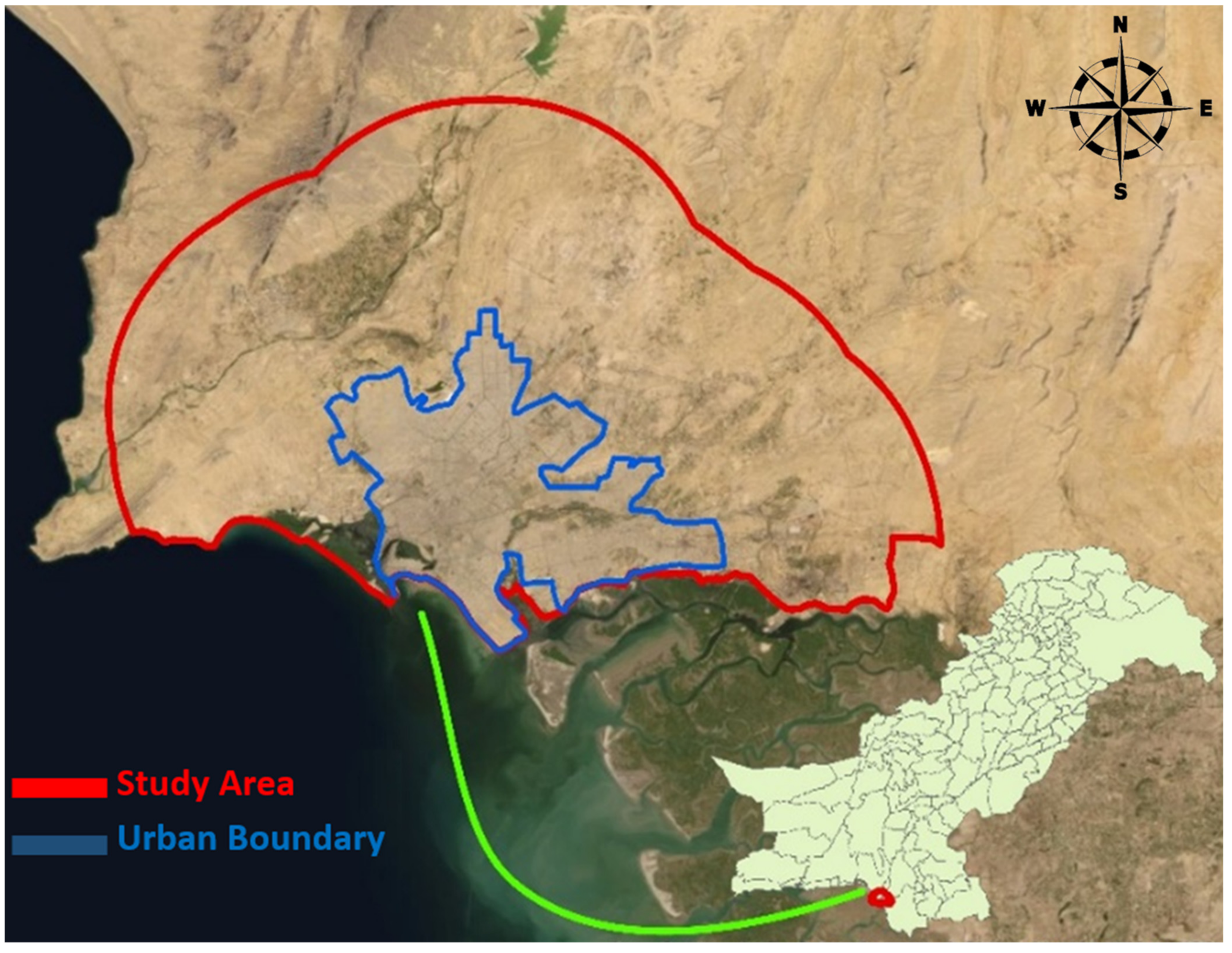
2. Study Area
3. Methodology
3.1. Data Acquisition
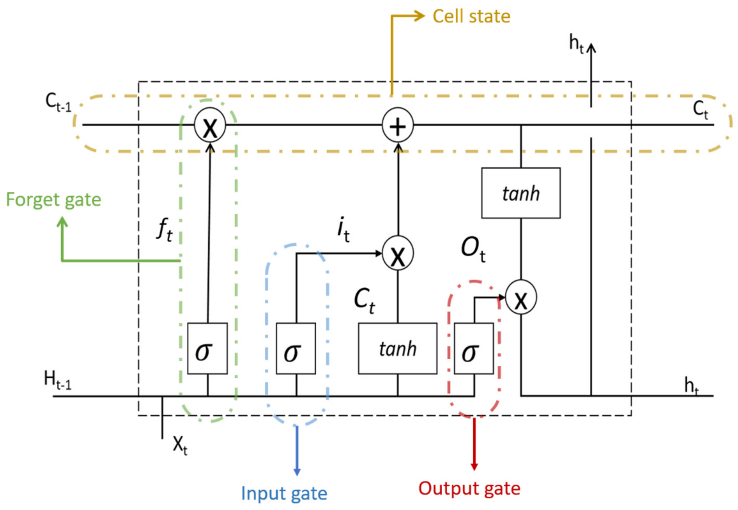
3.2. LSTM Network Development
- X = Element/point-wise multiplication
- + = Element/point-wise addition
- Tanh = Hyperbolic tangent
- σ = Sigmoid
- = input vector
- = output vector
- = sigmoid
- = weights
- = deviation matrices
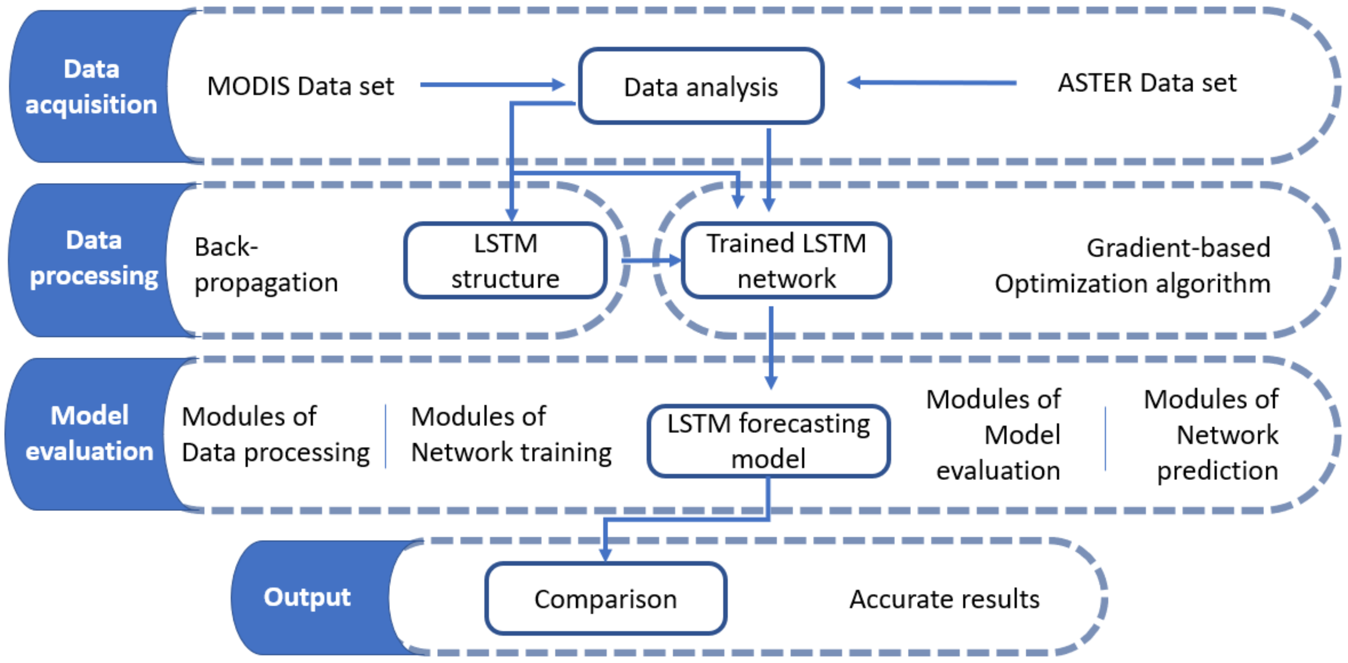
3.3. LSTM Forecasting Model
4. Results and Discussion
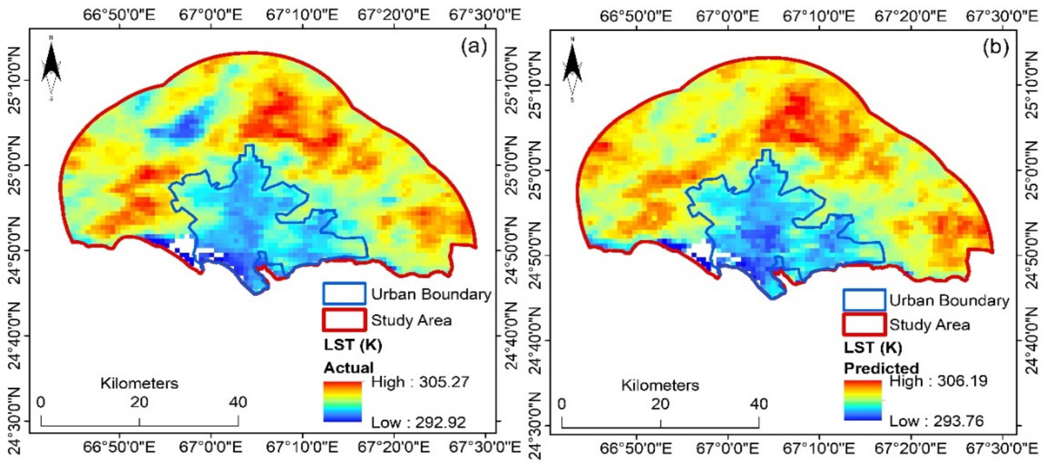
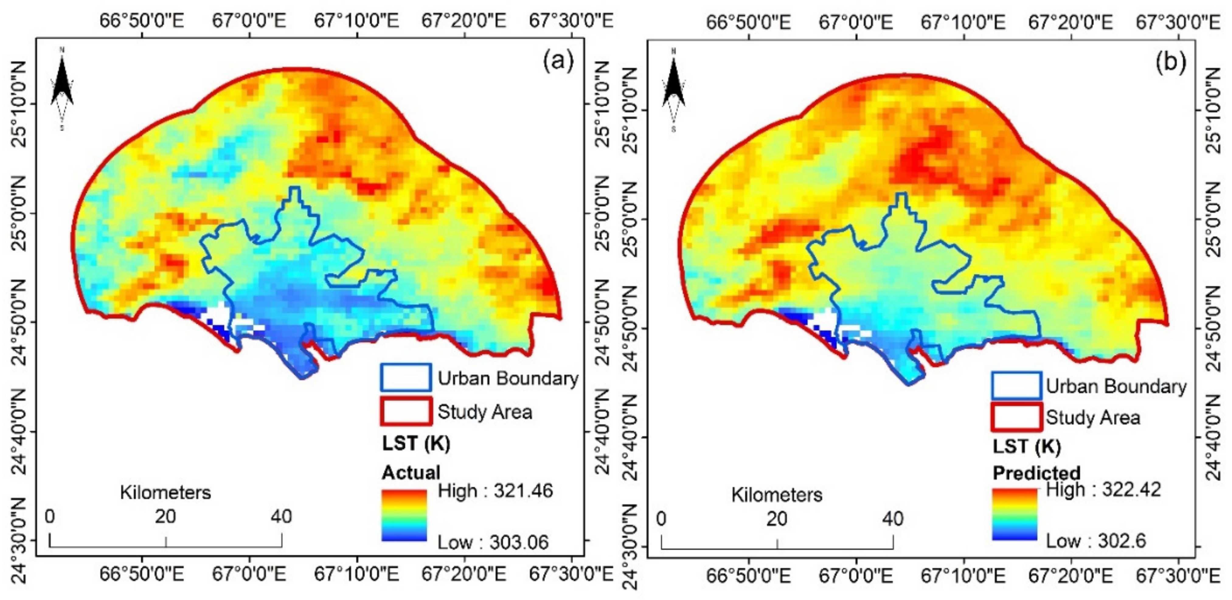
4.1. Land Surface Temperature (LST)
4.2. Enhanced Vegetation Index (EVI)
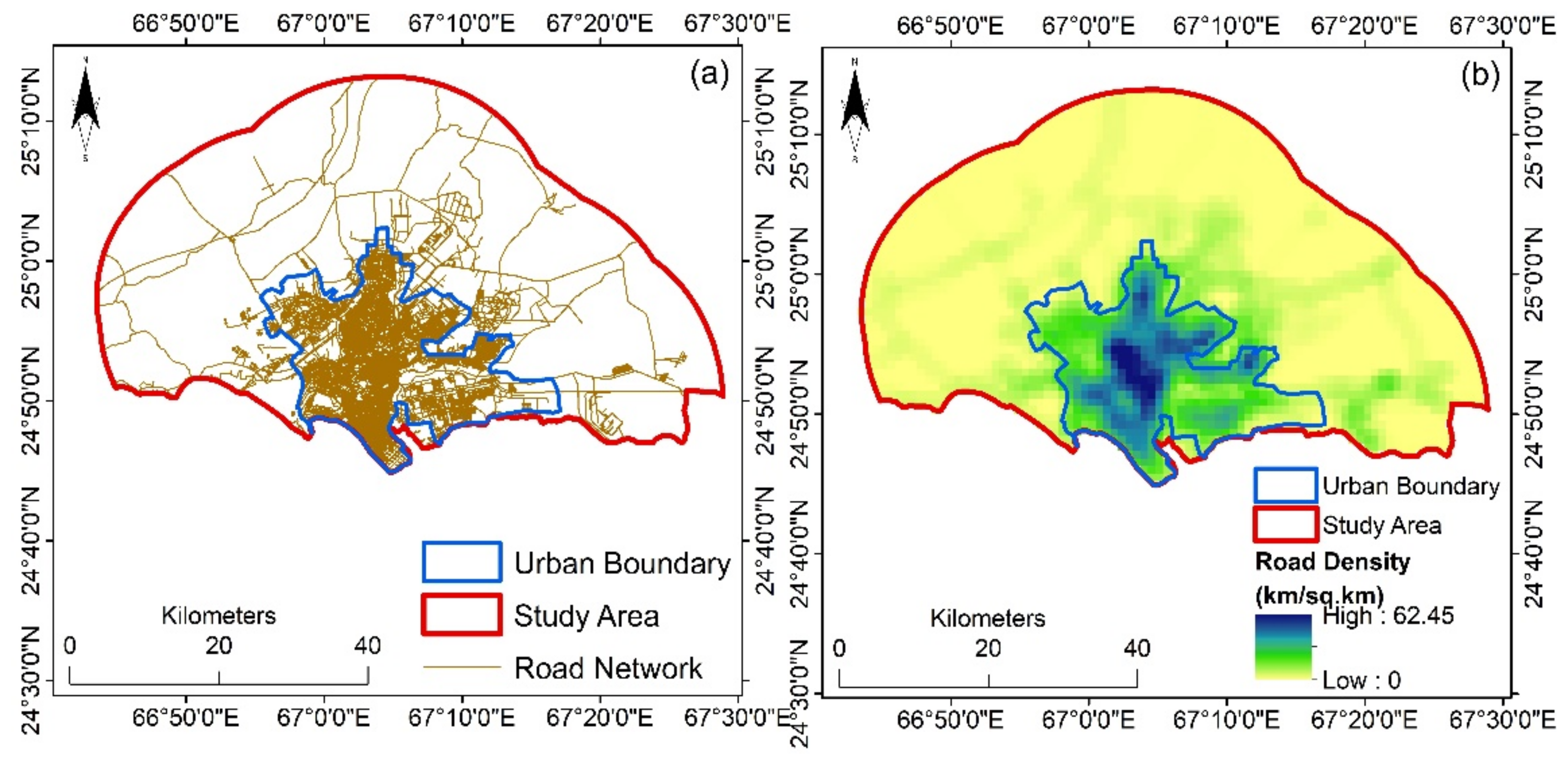
4.3. Road Density (RD)
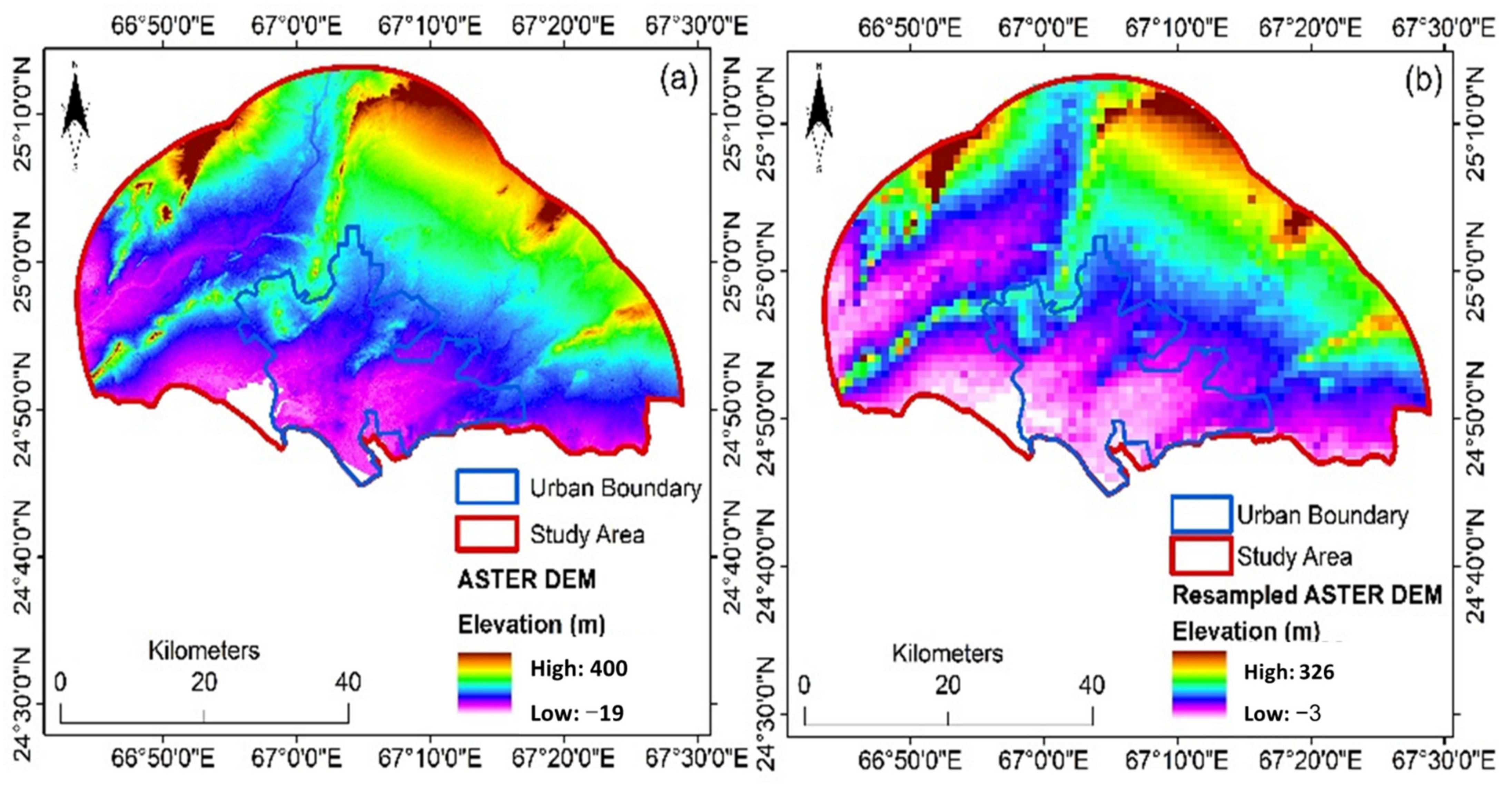
4.4. Elevation
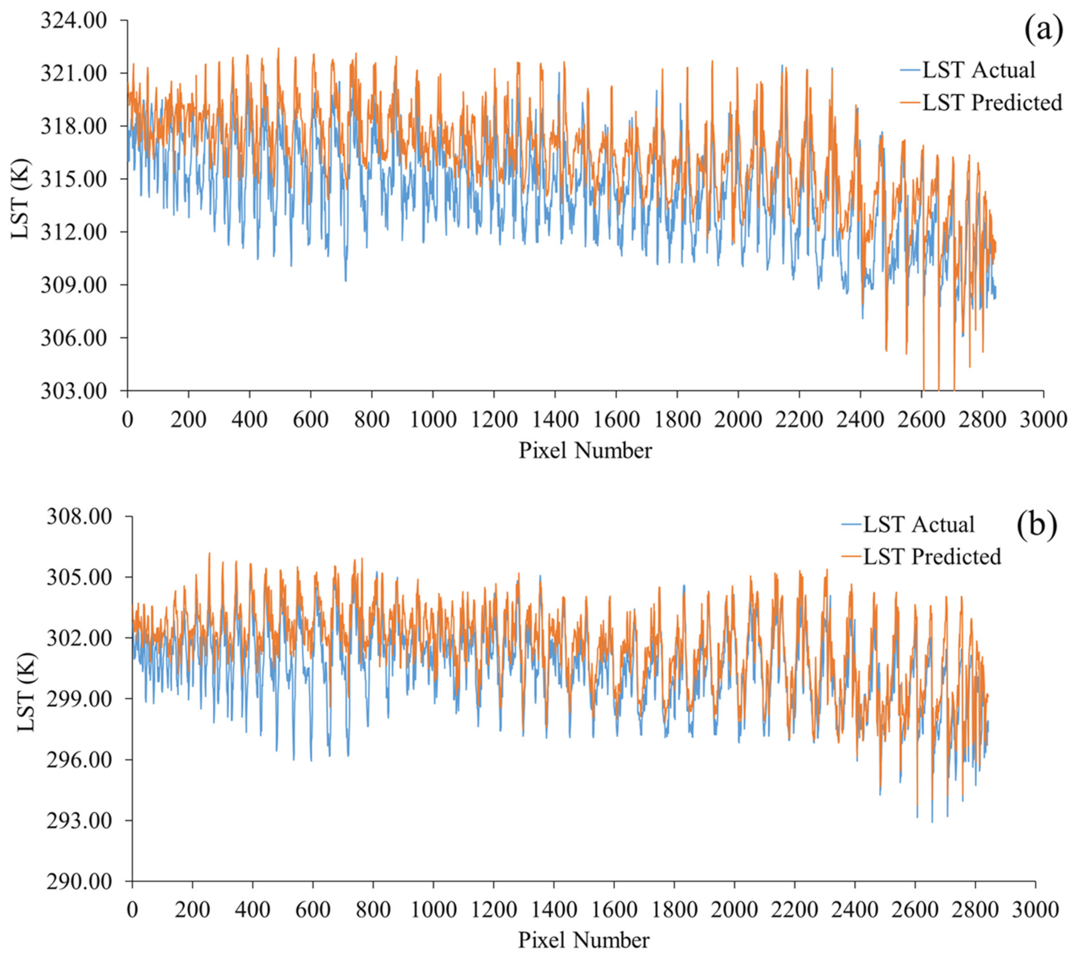
4.5. Model Validation
5. Conclusions
Author Contributions
Funding
Institutional Review Board Statement
Informed Consent Statement
Data Availability Statement
Conflicts of Interest
References
- Voogt, J.A.; Oke, T.R. Thermal remote sensing of urban climates. Remote Sens. Environ. 2003, 86, 370–384. [Google Scholar] [CrossRef]
- Grimm, N.B.; Faeth, S.H.; Golubiewski, N.E.; Redman, C.L.; Wu, J.; Bai, X.; Briggs, J.M. Global change and the ecology of cities. Sciences 2008, 319, 756–760. [Google Scholar] [CrossRef] [PubMed]
- Arshad, A.; Ashraf, M.; Sundari, R.S.; Qamar, H.; Wajid, M.; Hasan, M.-U. Vulnerability assessment of urban expansion and modelling green spaces to build heat waves risk resiliency in Karachi. Int. J. Disaster Risk Reduct. 2020, 46, 101468. [Google Scholar] [CrossRef]
- Landsberg, H.E. The Urban Climate; Academic Press: Cambridge, MA, USA, 1981. [Google Scholar]
- Santamouris, M.; Kolokotsa, D. On the impact of urban overheating and extreme climatic conditions on housing, energy, comfort and environmental quality of vulnerable population in Europe. Energy Build. 2015, 98, 125–133. [Google Scholar] [CrossRef]
- Streutker, D.R. A remote sensing study of the urban heat island of Houston, Texas. Int. J. Remote Sens. 2002, 23, 2595–2608. [Google Scholar] [CrossRef]
- Tran, H.; Uchihama, D.; Ochi, S.; Yasuoka, Y. Geoinformation. Assessment with satellite data of the urban heat island effects in Asian mega cities. Int. J. Appl. Earth Obs. Geoinf. 2006, 8, 34–48. [Google Scholar] [CrossRef]
- Tiangco, M.; Lagmay, A.; Argete, J. ASTER-based study of the night-time urban heat island effect in Metro Manila. Int. J. Remote Sens. 2008, 29, 2799–2818. [Google Scholar] [CrossRef]
- Cheval, S.; Dumitrescu, A. The July urban heat island of Bucharest as derived from MODIS images. Theor. Appl. Clim. 2009, 96, 145–153. [Google Scholar] [CrossRef]
- Mathew, A.; Sreekumar, S.; Khandelwal, S.; Kaul, N.; Kumar, R. Prediction of surface temperatures for the assessment of urban heat island effect over Ahmedabad city using linear time series model. Energy Build. 2016, 128, 605–616. [Google Scholar] [CrossRef]
- Akbari, H. Energy Saving Potentials and Air Quality Benefits of Urban Heat Island Mitigation. Lawrence Berkeley National Laboratory. 2005. Available online: https://escholarship.org/uc/item/4qs5f42s (accessed on 11 August 2021).
- Sarrat, C.; Lemonsu, A.; Masson, V.; Guedalia, D. Impact of urban heat island on regional atmospheric pollution. Atmos. Environ. 2006, 40, 1743–1758. [Google Scholar] [CrossRef]
- Taha, H. Urban climates and heat islands: Albedo, evapotranspiration, and anthropogenic heat. Energy Build. 1997, 25, 99–103. [Google Scholar] [CrossRef]
- Gray, K.A.; Finster, M.E. Northwestern University, Evanston, IL. The Urban Heat Island, Photochemical Smog, and Chicago: Local Features of the Problem and Solution; Atmospheric Pollution Prevention Division U.S. Environmental Protection Agency: Washington, DC, USA, 2000. [Google Scholar]
- Mirzaei, P.A.; Haghighat, F. A novel approach to enhance outdoor air quality: Pedestrian ventilation system. Build. Environ. 2010, 45, 1582–1593. [Google Scholar] [CrossRef]
- Monteiro, F.F.; Gonçalves, W.A.; Andrade, L.d.M.B.; Villavicencio, L.M.M.; dos Santos Silva, C.M. Assessment of Urban Heat Islands in Brazil based on MODIS remote sensing data. Urban Clim. 2021, 35, 100726. [Google Scholar] [CrossRef]
- Pu, R.; Gong, P.; Michishita, R.; Sasagawa, T. Assessment of multi-resolution and multi-sensor data for urban surface temperature retrieval. Remote Sens. Environ. 2006, 104, 211–225. [Google Scholar] [CrossRef]
- Mathew, A.; Khandelwal, S.; Kaul, N. Investigating spatio-temporal surface urban heat island growth over Jaipur city using geospatial techniques. Sustain. Cities Soc. 2018, 40, 484–500. [Google Scholar] [CrossRef]
- Yuan, F.; Bauer, M.E. Comparison of impervious surface area and normalized difference vegetation index as indicators of surface urban heat island effects in Landsat imagery. Remote Sens. Environ. 2007, 106, 375–386. [Google Scholar] [CrossRef]
- Bhattacharya, B.; Mallick, K.; Patel, N.; Parihar, J. Regional clear sky evapotranspiration over agricultural land using remote sensing data from Indian geostationary meteorological satellite. J. Hydrol. 2010, 387, 65–80. [Google Scholar] [CrossRef]
- Lakshmi, V.; Hong, S.; Small, E.E.; Chen, F. The influence of the land surface on hydrometeorology and ecology: New advances from modeling and satellite remote sensing. Hydrol. Res. 2011, 42, 95–112. [Google Scholar] [CrossRef]
- Zhangyan, J.; Yunhao, C.; Jing, L. On urban heat island of Beijing based on Landsat TM data. Geo-Spat. Inf. Sci. 2006, 9, 293–297. [Google Scholar] [CrossRef]
- Jusuf, S.K.; Wong, N.H.; Hagen, E.; Anggoro, R.; Hong, Y. The influence of land use on the urban heat island in Singapore. Habitat Int. 2007, 31, 232–242. [Google Scholar] [CrossRef]
- Liang, B.; Weng, Q. Development. Multiscale analysis of census-based land surface temperature variations and determinants in Indianapolis, United States. J. Urban Plan. Dev. 2008, 134, 129–139. [Google Scholar] [CrossRef]
- Munawar, H.S.; Ullah, F.; Khan, S.I.; Qadir, Z.; Qayyum, S. UAV Assisted Spatiotemporal Analysis and Management of Bushfires: A Case Study of the 2020 Victorian Bushfires. Fire 2021, 4, 40. [Google Scholar] [CrossRef]
- Mathew, A.; Sreekumar, S.; Khandelwal, S.; Kumar, R. Prediction of land surface temperatures for surface urban heat island assessment over Chandigarh city using support vector regression model. Sol. Energy 2019, 186, 404–415. [Google Scholar] [CrossRef]
- Zhang, K.; Wang, R.; Shen, C.; Da, L. Temporal and spatial characteristics of the urban heat island during rapid urbanization in Shanghai, China. Environ. Monit. Assess. 2010, 169, 101–112. [Google Scholar] [CrossRef]
- Parida, B.; Oinam, B.; Patel, N.; Sharma, N.; Kandwal, R.; Hazarika, M. Land surface temperature variation in relation to vegetation type using MODIS satellite data in Gujarat state of India. Int. J. Remote Sens. 2008, 29, 4219–4235. [Google Scholar] [CrossRef]
- Mathew, A.; Khandelwal, S.; Kaul, N. Analysis of diurnal surface temperature variations for the assessment of surface urban heat island effect over Indian cities. Energy Build. 2018, 159, 271–295. [Google Scholar] [CrossRef]
- Yang, S.; Wang, S. The effect of the afforestation trees in lowering temperatures and enhancing humidity of the air in Guangzhou. Geographical Series III. J. South China Norm. Univ. 1989, 1, 41–46. [Google Scholar]
- Goward, S.N.; Xue, Y.; Czajkowski, K.P. Evaluating land surface moisture conditions from the remotely sensed temperature/vegetation index measurements: An exploration with the simplified simple biosphere model. Remote Sens. Environ. 2002, 79, 225–242. [Google Scholar] [CrossRef]
- Weng, Q.; Lu, D.; Schubring, J. Estimation of land surface temperature–vegetation abundance relationship for urban heat island studies. Remote Sens. Environ. 2004, 89, 467–483. [Google Scholar] [CrossRef]
- Huete, A.; Justice, C.; Van Leeuwen, W. MODIS Vegetation Index (MOD 13) Algorithm Theoretical Basis Document, Version 3; National Aeronautics and Space Administration (NASA): Washington, DC, USA, 1999; Volume 1200.
- Khandelwal, S.; Goyal, R. Effect of vegetation and urbanization over land surface temperature: Case study of Jaipur City. In Proceedings of the EARSeL Symposium, Paris, France, 31 May–3 June 2010; pp. 177–183. [Google Scholar]
- Dousset, B.; Gourmelon, F. Satellite multi-sensor data analysis of urban surface temperatures and landcover. ISPRS J. Photogramm. Remote Sens. 2003, 58, 43–54. [Google Scholar] [CrossRef]
- Zhang, X.; Zhong, T.; Feng, X.; Wang, K. Estimation of the relationship between vegetation patches and urban land surface temperature with remote sensing. Int. J. Remote Sens. 2009, 30, 2105–2118. [Google Scholar] [CrossRef]
- Goyal, R.; Khandelwal, S.; Kaul, N. Analysis of relative importance of parameters representing vegetation, urbanization and elevation with land surface temperature using ANN. In Proceedings of the Geospatial World Forum Hyderabad, Hyderabad, India, 18–21 January 2011. [Google Scholar]
- United States Environmental Protection Agency. Heat Island Compendium. Available online: https://www.epa.gov/heatislands/heat-island-compendium (accessed on 29 July 2021).
- Battista, G.; de Lieto Vollaro, R.; Zinzi, M. Assessment of urban overheating mitigation strategies in a square in Rome, Italy. Sol. Energy 2019, 180, 608–621. [Google Scholar] [CrossRef]
- Teferi, E.; Abraha, H. Urban heat island effect of Addis Ababa City: Implications of urban green spaces for climate change adaptation. In Climate Change Adaptation in Africa; Springer: Berlin/Heidelberg, Germany, 2017; pp. 539–552. [Google Scholar]
- Estoque, R.C.; Murayama, Y. Monitoring surface urban heat island formation in a tropical mountain city using Landsat data (1987–2015). ISPRS J. Photogramm. Remote Sens. 2017, 133, 18–29. [Google Scholar] [CrossRef]
- Ranagalage, M.; Dissanayake, D.; Murayama, Y.; Zhang, X.; Estoque, R.C.; Perera, E.; Morimoto, T. Quantifying surface urban heat island formation in the world heritage tropical mountain city of Sri Lanka. ISPRS Int. J. Geo-Inf. 2018, 7, 341. [Google Scholar] [CrossRef]
- Estoque, R.C.; Murayama, Y.; Myint, S.W. Effects of landscape composition and pattern on land surface temperature: An urban heat island study in the megacities of Southeast Asia. Sci. Total Environ. 2017, 577, 349–359. [Google Scholar] [CrossRef]
- Simwanda, M.; Ranagalage, M.; Estoque, R.C.; Murayama, Y. Spatial analysis of surface urban heat islands in four rapidly growing African cities. Remote Sens. 2019, 11, 1645. [Google Scholar] [CrossRef]
- Priyankara, P.; Ranagalage, M.; Dissanayake, D.; Morimoto, T.; Murayama, Y. Spatial process of surface urban heat island in rapidly growing Seoul metropolitan area for sustainable urban planning using Landsat data (1996–2017). Climate 2019, 7, 110. [Google Scholar] [CrossRef]
- Cao, J.; Zhou, W.; Wang, J.; Hu, X.; Yu, W.; Zheng, Z.; Wang, W. Significant increase in extreme heat events along an urban–rural gradient. Landsc. Urban Plan. 2021, 215, 104210. [Google Scholar] [CrossRef]
- Dissanayake, D.; Morimoto, T.; Murayama, Y.; Ranagalage, M. Impact of landscape structure on the variation of land surface temperature in sub-saharan region: A case study of Addis Ababa using Landsat data (1986–2016). Sustainability 2019, 11, 2257. [Google Scholar] [CrossRef]
- Xiao, R.-B.; Ouyang, Z.-Y.; Zheng, H.; Li, W.-F.; Schienke, E.W.; Wang, X.-K. Spatial pattern of impervious surfaces and their impacts on land surface temperature in Beijing, China. J. Environ. Sci. 2007, 19, 250–256. [Google Scholar] [CrossRef]
- Myint, S.W.; Brazel, A.; Okin, G.; Buyantuyev, A. Combined effects of impervious surface and vegetation cover on air temperature variations in a rapidly expanding desert city. GISci. Remote Sens. 2010, 47, 301–320. [Google Scholar] [CrossRef]
- Ashtiani, A.; Mirzaei, P.A.; Haghighat, F. Indoor thermal condition in urban heat island: Comparison of the artificial neural network and regression methods prediction. Energy Build. 2014, 76, 597–604. [Google Scholar] [CrossRef]
- Ullah, F.; Al-Turjman, F.; Qayyum, S.; Inam, H.; Imran, M. Advertising through UAVs: Optimized path system for delivering smart real-estate advertisement materials. Int. J. Intell. Syst. 2021, 36, 3429–3463. [Google Scholar] [CrossRef]
- Munawar, H.S.; Ullah, F.; Qayyum, S.; Khan, S.I.; Mojtahedi, M. UAVs in Disaster Management: Application of Integrated Aerial Imagery and Convolutional Neural Network for Flood Detection. Sustainability 2021, 13, 7547. [Google Scholar] [CrossRef]
- Ma, X.; Tao, Z.; Wang, Y.; Yu, H.; Wang, Y. Long short-term memory neural network for traffic speed prediction using remote microwave sensor data. Transp. Res. Part C Emerg. Technol. 2015, 54, 187–197. [Google Scholar] [CrossRef]
- Aslam, B.; Ismail, S.; Maqsoom, A. Geospatial mapping of Tsunami susceptibility of Karachi to Gwadar coastal area of Pakistan. Arab. J. Geosci. 2020, 13, 894. [Google Scholar] [CrossRef]
- Alam, K.; Trautmann, T.; Blaschke, T. Aerosol optical properties and radiative forcing over mega-city Karachi. Atmos. Res. 2011, 101, 773–782. [Google Scholar] [CrossRef]
- Raza, D.; Karim, R.; Nasir, A.; Khan, S.; Zubair, M.H. Satellite Based Surveillance of LULC with Deliberation on Urban Land Surface Temperature and Precipitation Pattern Changes of Karachi. Pakistan. J. Geogr. Nat. Disast. 2019, 9, 1000237. [Google Scholar]
- Ghumman, U.; Horney, J. Characterizing the impact of extreme heat on mortality, Karachi, Pakistan, June 2015. Prehospital Disaster Med. 2016, 31, 263. [Google Scholar] [CrossRef] [PubMed]
- Salim, A.; Ahmed, A.; Ashraf, N.; Ashar, M. Deadly Heat Wavein Karachi, July 2015: Negligence or Mismanagement? Int. J. Occup. Environ. Med. 2015, 6, 249. [Google Scholar] [CrossRef][Green Version]
- Ullah, F.; Qayyum, S.; Thaheem, M.J.; Al-Turjman, F.; Sepasgozar, S.M. Risk management in sustainable smart cities governance: A TOE framework. Technol. Forecast. Soc. Chang. 2021, 167, 120743. [Google Scholar] [CrossRef]
- Atif, S.; Umar, M.; Ullah, F. Investigating the flood damages in Lower Indus Basin since 2000: Spatiotemporal analyses of the major flood events. Nat. Hazards 2021, 108, 1–27. [Google Scholar] [CrossRef]
- Hanif, U. Socio-economic impacts of heat wave in Sindh. Pak. J. Meteorol. 2017, 13, 87–96. [Google Scholar]
- Nasim, W.; Amin, A.; Fahad, S.; Awais, M.; Khan, N.; Mubeen, M.; Wahid, A.; Rehman, M.H.; Ihsan, M.Z.; Ahmad, S. Future risk assessment by estimating historical heat wave trends with projected heat accumulation using SimCLIM climate model in Pakistan. Atmos. Res. 2018, 205, 118–133. [Google Scholar] [CrossRef]
- Jing, R.; Liu, S.; Gong, Z.; Wang, Z.; Guan, H.; Gautam, A.; Zhao, W. Object-based change detection for VHR remote sensing images based on a Trisiamese-LSTM. Int. J. Remote Sens. 2020, 41, 6209–6231. [Google Scholar] [CrossRef]
- Li, X.-M.; Ma, Y.; Leng, Z.-H.; Zhang, J.; Lu, X.-X. High-accuracy remote sensing water depth retrieval for coral islands and reefs based on LSTM neural network. J. Coast. Res. 2020, 102, 21–32. [Google Scholar] [CrossRef]
- de Macedo, M.M.G.; Mattos, A.B.; Oliveira, D.A.B. Generalization of Convolutional LSTM Models for Crop Area Estimation. IEEE J. Sel. Top. Appl. Earth Obs. Remote Sens. 2020, 13, 1134–1142. [Google Scholar] [CrossRef]
- Wang, Y.; Gu, L.; Li, X.; Ren, R. Building Extraction in Multitemporal High-Resolution Remote Sensing Imagery Using a Multifeature LSTM Network. IEEE Geosci. Remote Sens. Lett. 2020, 1–5. [Google Scholar] [CrossRef]
- Qadir, Z.; Ullah, F.; Munawar, H.S.; Al-Turjman, F. Addressing disasters in smart cities through UAVs path planning and 5G communications: A systematic review. Comput. Commun. 2021, 168, 114–135. [Google Scholar] [CrossRef]
- Kafy, A.A.; Abdullah Al, F.; Rahman, M.S.; Islam, M.; Al Rakib, A.; Islam, M.A.; Khan, M.H.H.; Sikdar, M.S.; Sarker, M.H.S.; Mawa, J.; et al. Prediction of seasonal urban thermal field variance index using machine learning algorithms in Cumilla, Bangladesh. Sustain. Cities Soc. 2021, 64, 102542. [Google Scholar] [CrossRef]
- Ranagalage, M.; Ratnayake, S.S.; Dissanayake, D.; Kumar, L.; Wickremasinghe, H.; Vidanagama, J.; Cho, H.; Udagedara, S.; Jha, K.K.; Simwanda, M. Spatiotemporal variation of urban heat islands for implementing nature-based solutions: A case study of Kurunegala, Sri Lanka. ISPRS Int. J. Geo-Inf. 2020, 9, 461. [Google Scholar] [CrossRef]
- Sarif, M.; Rimal, B.; Stork, N.E. Assessment of changes in land use/land cover and land surface temperatures and their impact on surface urban heat island phenomena in the Kathmandu Valley (1988–2018). ISPRS Int. J. Geo-Inf. 2020, 9, 726. [Google Scholar] [CrossRef]
- Nurwanda, A.; Honjo, T. The prediction of city expansion and land surface temperature in Bogor City, Indonesia. Sustain. Cities Soc. 2020, 52, 101772. [Google Scholar] [CrossRef]
- Memon, R.; Leung, D.; Liu, C.-H. An investigation of urban heat island intensity (SUHII) as an indicator of urban heating. Atmos. Res. 2009, 94, 491–500. [Google Scholar] [CrossRef]
- Gui, X.; Wang, L.; Yao, R.; Yu, D.; Li, C. Investigating the urbanization process and its impact on vegetation change and urban heat island in Wuhan, China. Environ. Sci. Pollut. Res. 2019, 26, 30808–30825. [Google Scholar] [CrossRef]
- Wang, Z.; Liu, X.; Wang, H.; Zheng, K.; Li, H.; Wang, G.; An, Z. Monitoring Vegetation Greenness in Response to Climate Variation along the Elevation Gradient in the Three-River Source Region of China. ISPRS Int. J. Geo-Inf. 2021, 10, 193. [Google Scholar] [CrossRef]
- Tan, Z.; Lau, K.K.-L.; Ng, E. Urban tree design approaches for mitigating daytime urban heat island effects in a high-density urban environment. Energy Build. 2016, 114, 265–274. [Google Scholar] [CrossRef]
- Lin, P.; Lau, S.S.Y.; Qin, H.; Gou, Z. Effects of urban planning indicators on urban heat island: A case study of pocket parks in high-rise high-density environment. Landsc. Urban Plan. 2017, 168, 48–60. [Google Scholar] [CrossRef]
- Wong, M.S.; Nichol, J.E.; To, P.H.; Wang, J. A simple method for designation of urban ventilation corridors and its application to urban heat island analysis. Build. Environ. 2010, 45, 1880–1889. [Google Scholar] [CrossRef]
- Hart, M.A.; Sailor, D.J. Quantifying the influence of land-use and surface characteristics on spatial variability in the urban heat island. Theor. Appl. Climatol. 2009, 95, 397–406. [Google Scholar] [CrossRef]
- Ge, X.; Mauree, D.; Castello, R.; Scartezzini, J.-L. Spatio-Temporal Relationship between Land Cover and Land Surface Temperature in Urban Areas: A Case Study in Geneva and Paris. ISPRS Int. J. Geo-Inf. 2020, 9, 593. [Google Scholar] [CrossRef]
- Yang, Y.; Lv, H.; Fu, Y.; He, X.; Wang, W. Associations between road density, urban forest landscapes, and structural-taxonomic attributes in northeastern china: Decoupling and implications. Forests 2019, 10, 58. [Google Scholar] [CrossRef]
- Khandelwal, S.; Goyal, R.; Kaul, N.; Mathew, A. Assessment of land surface temperature variation due to change in elevation of area surrounding Jaipur, India. Egypt. J. Remote Sens. Space Sci. 2018, 21, 87–94. [Google Scholar] [CrossRef]
- Liu, W.; Ji, C.; Zhong, J.; Jiang, X.; Zheng, Z. Temporal characteristics of the Beijing urban heat island. Theor. Appl. Clim. 2007, 87, 213–221. [Google Scholar] [CrossRef]


| Remote Sensing Product | Short Name | Sensor | Platform | Temporal Resolution | Spatial Resolution (m) |
|---|---|---|---|---|---|
| Land Surface Temperature and Emissivity | MYD11A2 | MODIS | Aqua | 8-day | 926.626 |
| Vegetation Indices | MYD13A2 | MODIS | Aqua | 16-day | 926.626 |
| Land Cover Type | MCD12Q1 | MODIS | Combined Aqua and Tera | Yearly | 463.3 |
| Digital Elevation Model | ASTGTM | ASTER | Terra | _ | 24.8 |
| Day No. | Maximum | Minimum | Mean | Standard Deviation | |
|---|---|---|---|---|---|
| January (009–016) | Actual | 292.92 | 305.27 | 296.42 | 1.289 |
| Predicted | 293.76 | 306.19 | 297.11 | 1.267 | |
| May (137–144) | Actual | 303.06 | 321.46 | 314.76 | 1.295 |
| Predicted | 302.6 | 322.42 | 314.89 | 1.326 | |
| Month | January | May |
|---|---|---|
| Day No. | 009–016 | 137–144 |
| MAE (K) | 0.27 | 0.29 |
| MAPE (%) | 0.15 | 0.13 |
| MSE | 0.237 | 0.261 |
| January | Between −3 to −2 K | Between −2 to −1 K | Between −1 to 0 K | Between 0 to 1 K | Between 1 to 2 K |
|---|---|---|---|---|---|
| Day No. 009–016 | 284 (6%) | 824 (9%) | 1307 (41%) | 256 (34%) | 171 (10%) |
| May | Between −2 to −1 K | Between −1 to 0 K | Between 0 to 1 K | Between 1 to 2 K | Between 2 to 3 K |
| Day No. 137–144 | 256 (9%) | 512 (18%) | 1279 (45%) | 284 (10%) | 512 (18%) |
Publisher’s Note: MDPI stays neutral with regard to jurisdictional claims in published maps and institutional affiliations. |
© 2021 by the authors. Licensee MDPI, Basel, Switzerland. This article is an open access article distributed under the terms and conditions of the Creative Commons Attribution (CC BY) license (https://creativecommons.org/licenses/by/4.0/).
Share and Cite
Aslam, B.; Maqsoom, A.; Khalid, N.; Ullah, F.; Sepasgozar, S. Urban Overheating Assessment through Prediction of Surface Temperatures: A Case Study of Karachi, Pakistan. ISPRS Int. J. Geo-Inf. 2021, 10, 539. https://doi.org/10.3390/ijgi10080539
Aslam B, Maqsoom A, Khalid N, Ullah F, Sepasgozar S. Urban Overheating Assessment through Prediction of Surface Temperatures: A Case Study of Karachi, Pakistan. ISPRS International Journal of Geo-Information. 2021; 10(8):539. https://doi.org/10.3390/ijgi10080539
Chicago/Turabian StyleAslam, Bilal, Ahsen Maqsoom, Nauman Khalid, Fahim Ullah, and Samad Sepasgozar. 2021. "Urban Overheating Assessment through Prediction of Surface Temperatures: A Case Study of Karachi, Pakistan" ISPRS International Journal of Geo-Information 10, no. 8: 539. https://doi.org/10.3390/ijgi10080539
APA StyleAslam, B., Maqsoom, A., Khalid, N., Ullah, F., & Sepasgozar, S. (2021). Urban Overheating Assessment through Prediction of Surface Temperatures: A Case Study of Karachi, Pakistan. ISPRS International Journal of Geo-Information, 10(8), 539. https://doi.org/10.3390/ijgi10080539