
Using Geomatic Techniques to Estimate Volume–Area Relationships of Watering Ponds


 ,
,  , and
, and 
Abstract
:1. Introduction
- To apply and compare different geomatic approaches and techniques to model the topography of small watering ponds (terrestrial or close-range SfM-MVS, aerial SfM-MVS, GNSS, LIDAR, and TLS). Specifically, the suitability of terrestrial SfM-MVS photogrammetry was tested, as it could be a low-cost, high-accuracy alternative to laser technologies or more time-consuming GNSS surveys. Tips on the use of this approach are also provided;
- To assess the overall suitability of power and quadratic functions to describe watering-pond geometry by means of pond-specific V–A–h relationships. These relationships could be a valuable tool to be used as a geometric model of watering ponds in hydrological simulation studies;
- To obtain a generalized V–A relationship from the surveys carried out at eight small watering ponds that may be used to estimate the storage capacity of other watering ponds in similar rangeland areas.
2. Materials and Methods
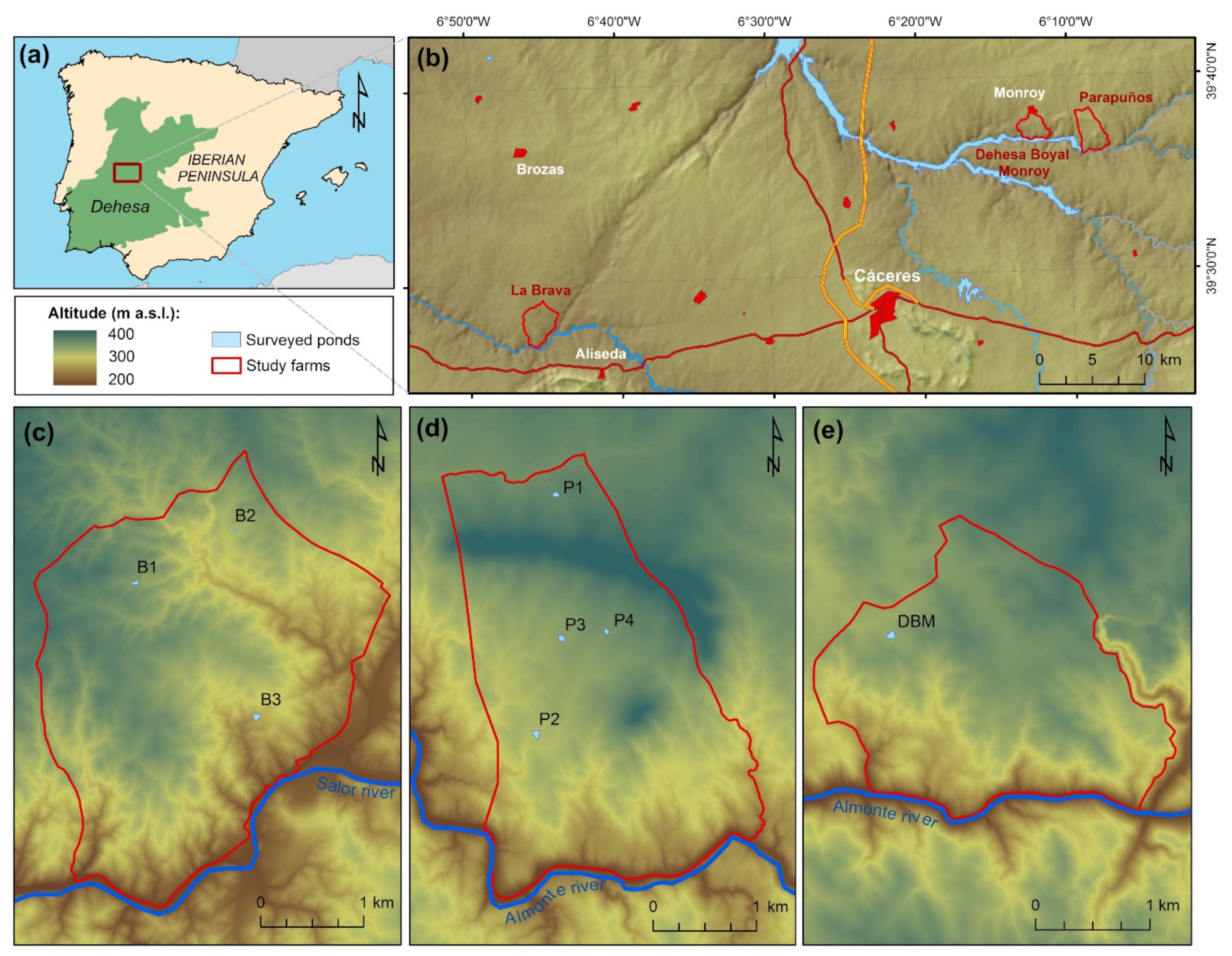
2.1. Study Area
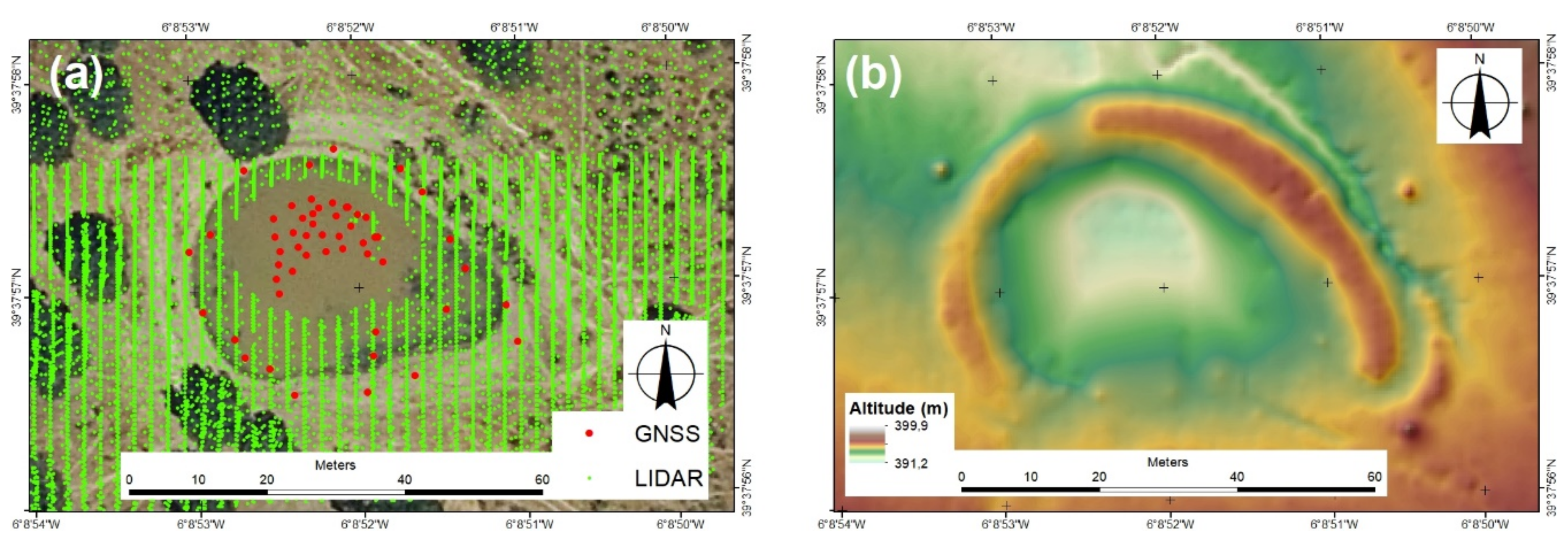
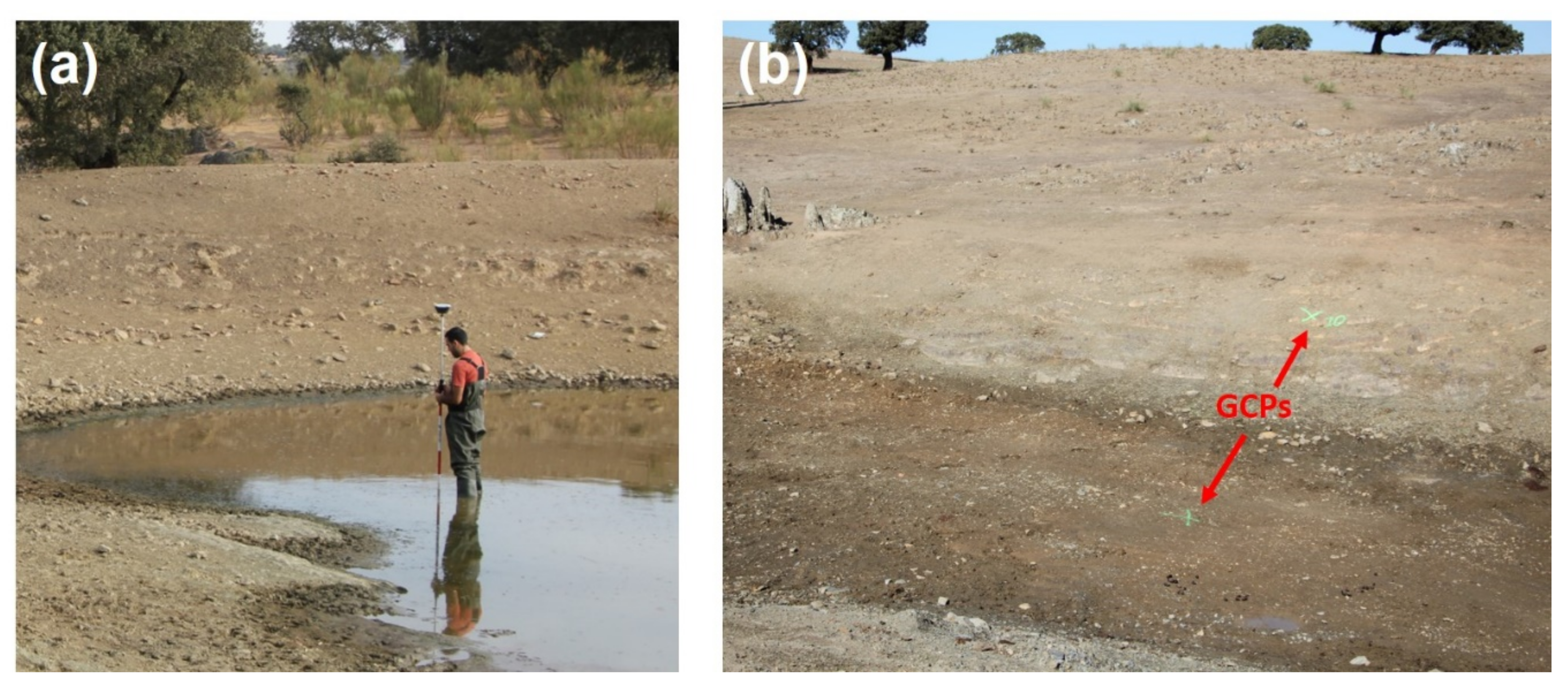
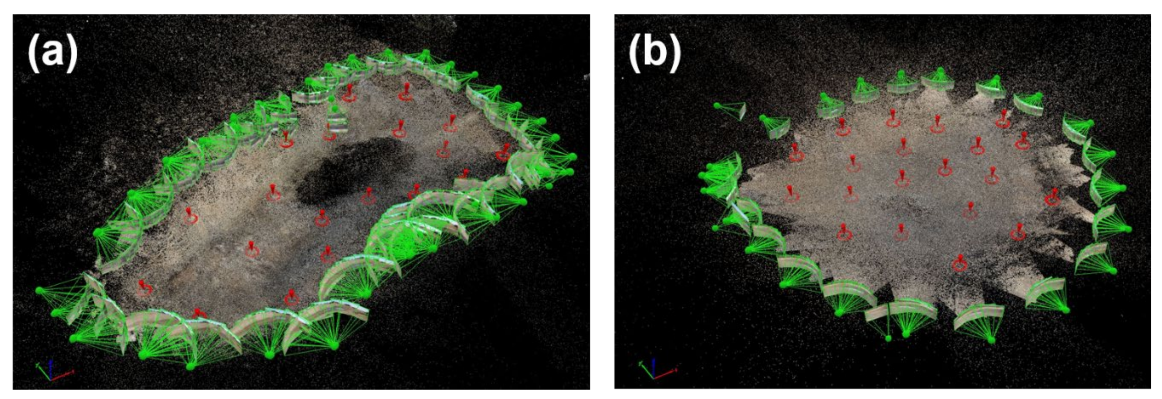
2.2. Surveying Watering-Pond Geometry
2.3. Obtaining Volume–Area–Height Relationships
3. Results
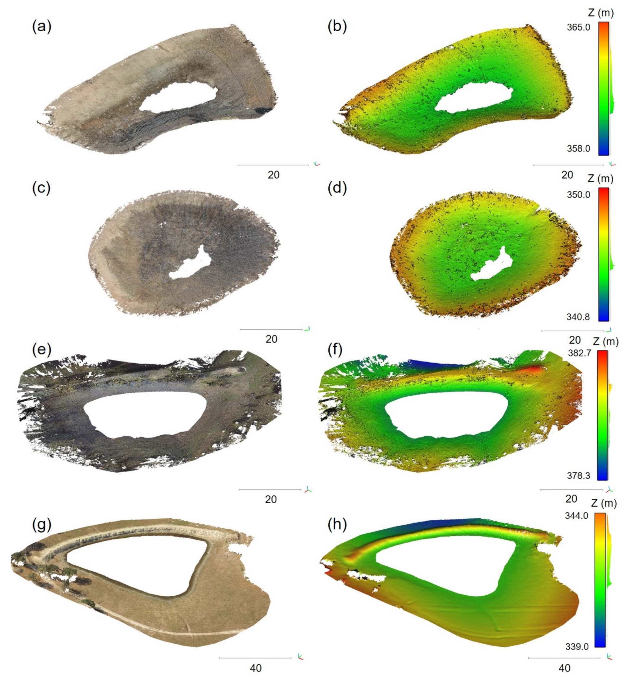
3.1. Suitability of Terrestrial and Aerial SfM-MVS Photogrammetry to Model the Topography of Small Watering Ponds
3.2. GNSS, TLS, and LIDAR
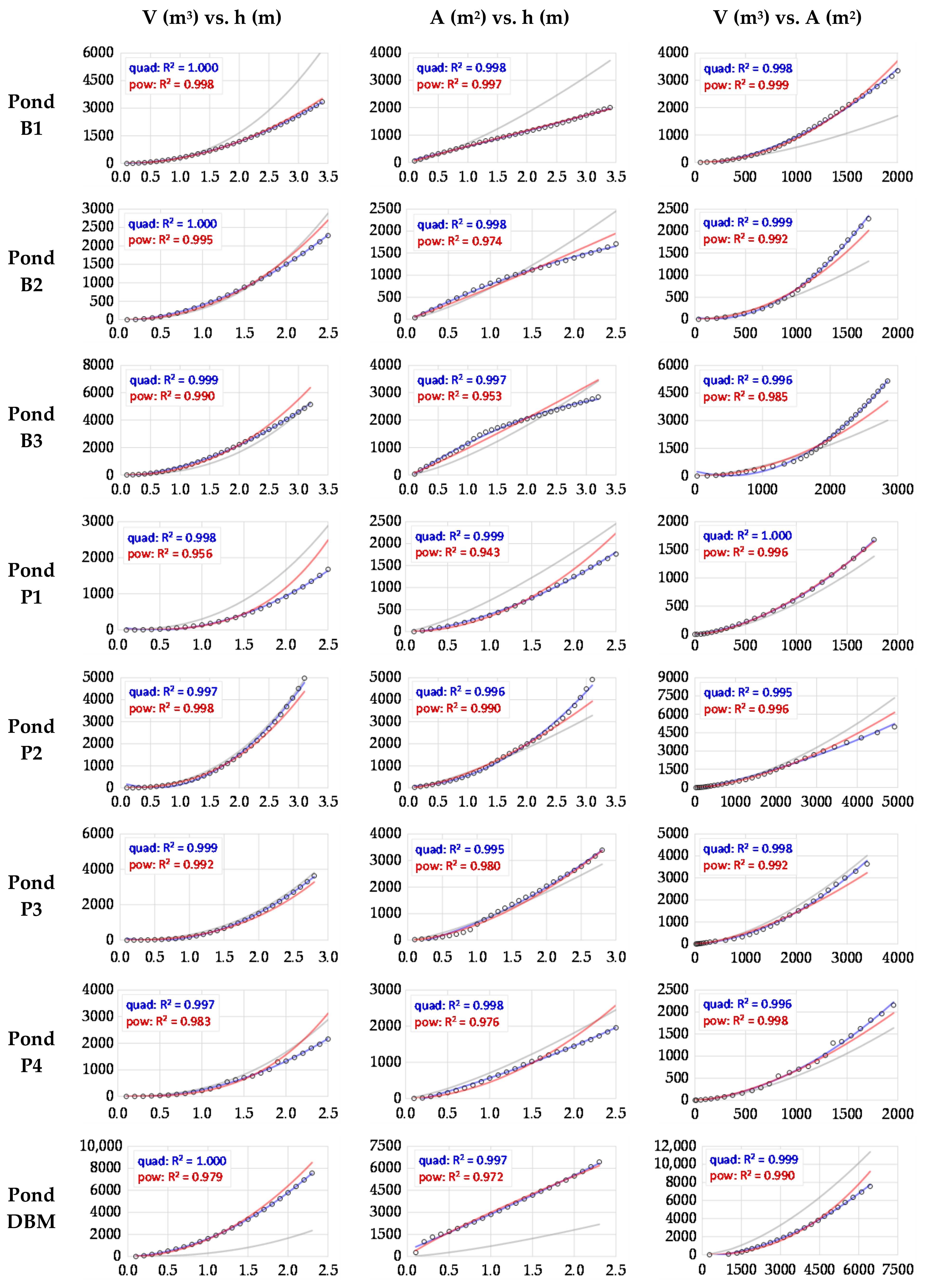
3.3. Pond-Specific and Generalized V–A–h Models
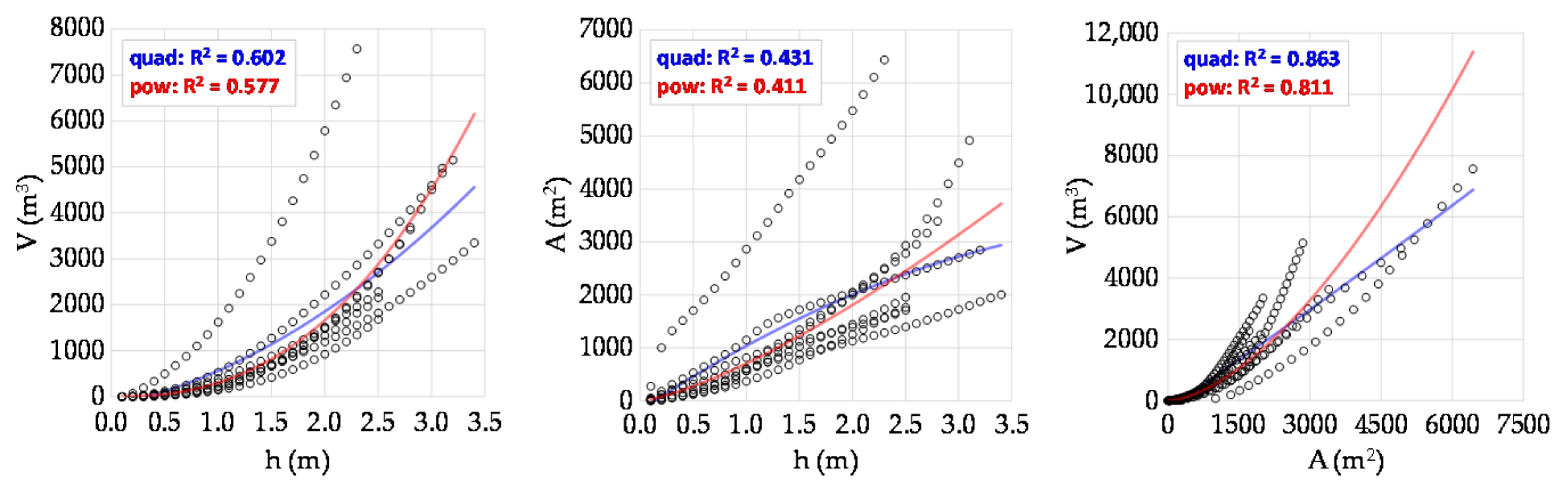
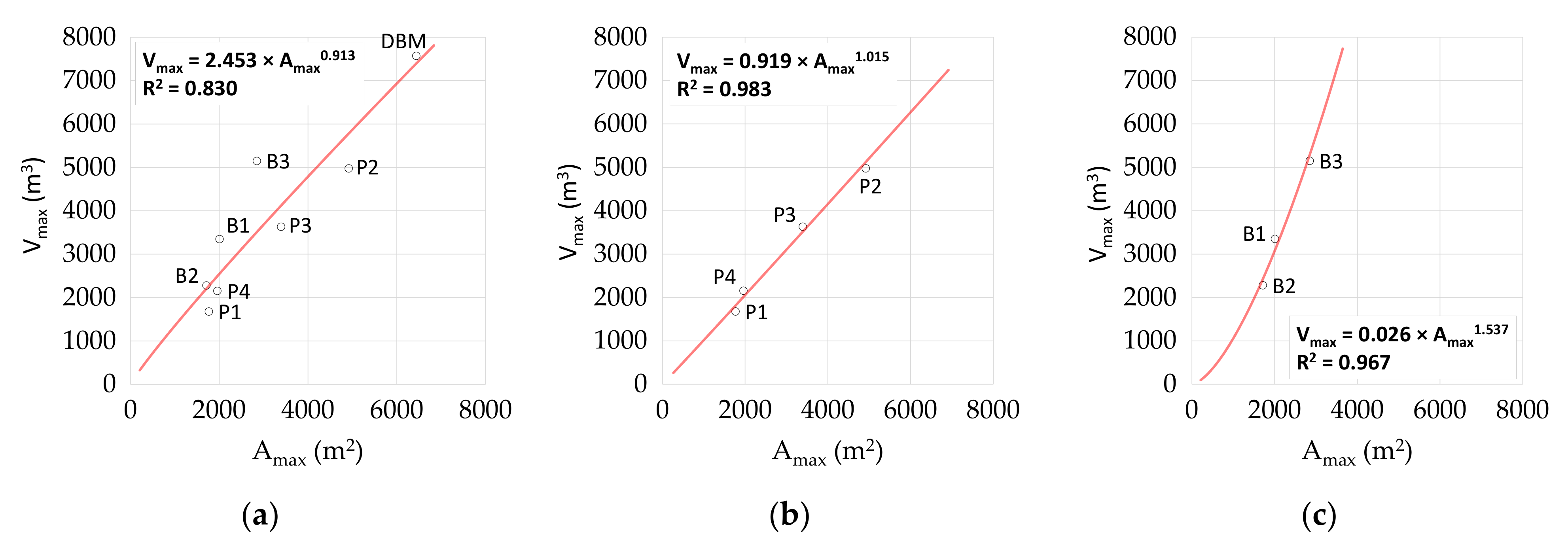
3.4. Generalized V–A Relationships for Estimating Water-Storage Capacity
4. Discussion
4.1. Suitability of V–A–h Models to Describe Watering Pond Morphometry
4.2. Performance of V–A Relationships for Estimating Water Storage Capacity in Watering Ponds
5. Conclusions
Author Contributions
Funding
Institutional Review Board Statement
Informed Consent Statement
Data Availability Statement
Conflicts of Interest
References
- Pulido-Fernández, M.; Schnabel, S. La disponibilidad de agua en explotaciones de ganadería extensiva. In Aportaciones a la Geografía Física de Extremadura con Especial Referencia a las Dehesas; Schnabel, S., Lavado-Contador, F., Gómez-Gutiérrez, A., García-Marín, R., Eds.; Fundicotex: Cáceres, Spain, 2010; pp. 221–235. (In Spanish) [Google Scholar]
- Camacho, J.; Sánchez, E.; Aguilar, F.; Gómez, A.; Lozano, A. Manual Práctico de Balsas Agrícolas. Diseño y Gestión Para su Mejora Ambiental; Consejería de Medio Ambiente (Junta de Andalucía): Sevilla, Spain, 2011. (In Spanish) [Google Scholar]
- Marín-Comitre, U.; Schnabel, S.; Pulido-Fernández, M. Hydrological Characterization of Watering Ponds in Rangeland Farms in the Southwest Iberian Peninsula. Water 2020, 12, 1038. [Google Scholar] [CrossRef] [Green Version]
- Rosenberry, D.O.; Hayashi, M. Assessing and Measuring Wetland Hydrology. In Wetland Techniques; Anderson, J.T., Davis, C.A., Eds.; Springer: Dordrecht, The Netherlands, 2013; Volume 1, pp. 87–225. [Google Scholar]
- Hayashi, M.; van der Kamp, G. Water level changes in ponds and lakes: The hydrological processes. In Plant Disturbance Ecology. The Process and the Response; Johnson, E.A., Miyanishi, K., Eds.; Academic Press: San Diego, CA, USA, 2007; pp. 311–339. [Google Scholar]
- O’Connor, D.J. Seasonal and long-term variations of dissolved solids in lakes and reservoirs. J. Environ. Eng. 1989, 115, 1213–1234. [Google Scholar] [CrossRef]
- Wise, W.R.; Annable, M.D.; Walser, J.A.E.; Switt, R.S.; Shaw, D.T. A wetland–aquifer interaction test. J. Hydrol. 2000, 227, 257–272. [Google Scholar] [CrossRef]
- Trigg, M.A.; Cook, P.G.; Brunner, P. Groundwater fluxes in a shallow seasonal wetland pond: The effect of bathymetric uncertainty on predicted water and solute balances. J. Hydrol. 2014, 517, 901–912. [Google Scholar] [CrossRef]
- Mishra, V.; Cherkauer, K.A.; Bowling, L.C. Parameterization of Lakes and Wetlands for Energy and Water Balance Studies in the Great Lakes Region. J. Hydrometeorol. 2010, 11, 1057–1082. [Google Scholar] [CrossRef]
- Liebe, J.R.; Van De Giesen, N.; Andreini, M.; Walter, M.T.; Steenhuis, T.S. Determining watershed response in data poor environments with remotely sensed small reservoirs as runoff gauges. Water Resour. Res. 2009, 45. [Google Scholar] [CrossRef] [Green Version]
- Hughes, D.A.; Mantel, S.K. Estimating the uncertainty in simulating the impacts of small farm dams on streamflow regimes in South Africa. Hydrol. Sci. J. 2010, 55, 578–592. [Google Scholar] [CrossRef]
- Gal, L.; Grippa, M.; Hiernaux, P.; Peugeot, C.; Mougin, E.; Kergoat, L. Changes in lakes water volume and runoff over ungauged Sahelian watersheds. J. Hydrol. 2016, 540, 1176–1188. [Google Scholar] [CrossRef]
- Ogilvie, A.; Belaud, G.; Massuel, S.; Mulligan, M.; Le Goulven, P.; Calvez, R. Assessing floods and droughts in ungauged small reservoirs with long-term landsat imagery. Geosciences 2016, 6, 42. [Google Scholar] [CrossRef] [Green Version]
- Neitsch, S.L.; Arnold, J.G.; Kiniry, J.R.; Williams, J.R. Soil and Water Assessment Tool: Theoretical documentation (Version 2009); Texas Water Resources Institute: College Station, TX, USA, 2011. [Google Scholar]
- Los Huertos, M.; Smith, D. Wetland bathymetry and mapping. In Wetland Techniques; Anderson, J.T., Davis, C.A., Eds.; Springer: Dordrecht, The Netherlands, 2013; Volume 1, pp. 49–86. [Google Scholar]
- Hohenthal, J.; Alho, P.; Hyyppä, J.; Hyyppä, H. Laser scanning applications in fluvial studies. Prog. Phys. Geogr. Earth Environ. 2011, 35, 782–809. [Google Scholar] [CrossRef]
- CNIG. Centro de descargas del Centro Nacional de Información Geográfica (CNIG). Ministerio de Transportes, Movilidad y Agenda Urbana, Government of Spain. (In Spanish). Available online: https://centrodedescargas.cnig.es/CentroDescargas/index.jsp (accessed on 4 June 2021).
- Langhammer, J.; Janský, B.; Kocum, J.; Minařík, R. 3-D reconstruction of an abandoned montane reservoir using UAV photogrammetry, aerial LiDAR and field survey. Appl. Geogr. 2018, 98, 9–21. [Google Scholar] [CrossRef]
- Rhee, D.S.; Kim, Y.D.; Kang, B.; Kim, D. Applications of unmanned aerial vehicles in fluvial remote sensing: An overview of recent achievements. KSCE J. Civ. Eng. 2018, 22, 588–602. [Google Scholar] [CrossRef]
- Rusnák, M.; Sládek, J.; Kidová, A.; Lehotský, M. Template for high-resolution river landscape mapping using UAV technology. Measurement 2018, 115, 139–151. [Google Scholar] [CrossRef]
- Bailly, J.-S.; Le Coarer, Y.; Languille, P.; Stigermark, C.-J.; Allouis, T. Geostatistical estimations of bathymetric LiDAR errors on rivers. Earth Surf. Process. Landf. 2010, 35, 1199–1210. [Google Scholar] [CrossRef]
- Raineault, N.A.; Trembanis, A.C.; Miller, D.C. Mapping Benthic Habitats in Delaware Bay and the Coastal Atlantic: Acoustic Techniques Provide Greater Coverage and High Resolution in Complex, Shallow-Water Environments. Estuaries Coasts 2012, 35, 682–699. [Google Scholar] [CrossRef]
- Smith, M.; Vericat, D.; Gibbins, C. Through-water terrestrial laser scanning of gravel beds at the patch scale. Earth Surf. Process. Landf. 2012, 37, 411–421. [Google Scholar] [CrossRef]
- Kurowski, M.; Thal, J.; Damerius, R.; Korte, H.; Jeinsch, T. Automated Survey in Very Shallow Water using an Unmanned Surface Vehicle. IFAC PapersOnLine 2019, 52, 146–151. [Google Scholar] [CrossRef]
- Burdziakowski, P.; Specht, C.; Dabrowski, P.S.; Specht, M.; Lewicka, O.; Makar, A. Using UAV Photogrammetry to Analyse Changes in the Coastal Zone Based on the Sopot Tombolo (Salient) Measurement Project. Sensors 2020, 20, 4000. [Google Scholar] [CrossRef] [PubMed]
- Genchi, S.A.; Vitale, A.J.; Perillo, G.M.E.; Seitz, C.; Delrieux, C.A. Mapping Topobathymetry in a Shallow Tidal Environment Using Low-Cost Technology. Remote Sens. 2020, 12, 1394. [Google Scholar] [CrossRef]
- Specht, M.; Specht, C.; Mindykowski, J.; Dąbrowski, P.; Maśnicki, R.; Makar, A. Geospatial Modeling of the Tombolo Phenomenon in Sopot using Integrated Geodetic and Hydrographic Measurement Methods. Remote Sens. 2020, 12, 737. [Google Scholar] [CrossRef] [Green Version]
- Stateczny, A.; Kazimierski, W.; Burdziakowski, P.; Motyl, W.; Wisniewska, M. Shore Construction Detection by Automotive Radar for the Needs of Autonomous Surface Vehicle Navigation. ISPRS Int. J. Geo Inf. 2019, 8, 80. [Google Scholar] [CrossRef] [Green Version]
- Kedzierski, M.; Wilińska, M.; Wierzbicki, D.; Fryskowska, A.; Deliś, P. Image data fusion for flood plain mapping. In Proceedings of the 9th International Conference Environmental Engineering (9th Icee)—Selected Papers, Vilnius, Lithuania, 22–23 May 2014. [Google Scholar] [CrossRef] [Green Version]
- Gao, H.; Birkett, C.; Lettenmaier, D.P. Global monitoring of large reservoir storage from satellite remote sensing. Water Resour. Res. 2012, 48. [Google Scholar] [CrossRef] [Green Version]
- Sima, S.; Tajrishy, M. Using satellite data to extract volume–area–elevation relationships for Urmia Lake, Iran. J. Great Lakes Res. 2013, 39, 90–99. [Google Scholar] [CrossRef]
- Song, C.; Huang, B.; Ke, L. Modeling and analysis of lake water storage changes on the Tibetan Plateau using multi-mission satellite data. Remote Sens. Environ. 2013, 135, 25–35. [Google Scholar] [CrossRef]
- Smith, L.C.; Pavelsky, T.M. Remote sensing of volumetric storage changes in lakes. Earth Surf. Process. Landf. 2009, 34, 1353–1358. [Google Scholar] [CrossRef]
- Lu, S.; Ouyang, N.; Wu, B.; Wei, Y.; Tesemma, Z. Lake water volume calculation with time series remote-sensing images. Int. J. Remote Sens. 2013, 34, 7962–7973. [Google Scholar] [CrossRef]
- Birkett, C.M. Synergistic remote sensing of Lake Chad Variability of basin inundation. Remote Sens. Environ. 2000, 72, 218–236. [Google Scholar] [CrossRef]
- Duan, Z.; Bastiaanssen, W.G.M. Estimating water volume variations in lakes and reservoirs from four operational satellite altimetry databases and satellite imagery data. Remote Sens. Environ. 2013, 134, 403–416. [Google Scholar] [CrossRef]
- Baup, F.; Frappart, F.; Maubant, J. Combining high-resolution satellite images and altimetry to estimate the volume of small lakes. Hydrol. Earth Syst. Sci. 2014, 18, 2007–2020. [Google Scholar] [CrossRef] [Green Version]
- De Graaf, G.; Kamal, M.; Martin, T.; Schepel, M. Remote sensing techniques for detecting and mapping aquaculture ponds in Bangladesh. In Proceedings of the Second International Symposium on GIS-Spatial Analyses in Fishery and Aquatic Sciences, Brighton, UK, 3–6 September 2002; pp. 3–6. [Google Scholar]
- Jones, K.; Lanthier, Y.; van der Voet, P.; van Valkengoed, E.; Taylor, D.; Fernández-Prieto, D. Monitoring and assessment of wetlands using Earth Observation: The GlobWetland project. J. Environ. Manag. 2009, 90, 2154–2169. [Google Scholar] [CrossRef]
- Gallant, A.L. The Challenges of Remote Monitoring of Wetlands. Remote Sens. 2015, 7, 10938–10950. [Google Scholar] [CrossRef] [Green Version]
- Ogilvie, A.; Belaud, G.; Massuel, S.; Mulligan, M.; Le Goulven, P.; Calvez, R. Surface water monitoring in small water bodies: Potential and limits of multi-sensor Landsat time series. Hydrol. Earth Syst. Sci. 2018, 22, 4349–4380. [Google Scholar] [CrossRef] [Green Version]
- Ullman, S. Interpretation of structure from motion. Proc. R. Soc. London Ser. B Biol. Sci. 1979, 203, 405–426. [Google Scholar] [CrossRef]
- Seitz, S.M.; Curless, B.; Diebel, J.; Scharstein, D.; Szeliski, R. A comparison and evaluation of multi-view stereo reconstruction algorithms. In Proceedings of the 2006 IEEE Computer Society Conference on Computer Vision and Pattern Recognition (CVPR’06), New York, NY, USA, 17–22 June 2006; pp. 519–528. [Google Scholar]
- Castillo, C.; Pérez, R.; James, M.R.; Quinton, J.N.; Taguas, E.V.; Gomez, J.A. Comparing the Accuracy of Several Field Methods for Measuring Gully Erosion. Soil Sci. Soc. Am. J. 2012, 76, 1319–1332. [Google Scholar] [CrossRef] [Green Version]
- Chandler, J.; Fryer, J. Autodesk 123D catch: How accurate is it. Geomat. World 2013, 2, 28–30. [Google Scholar]
- Fonstad, M.A.; Dietrich, J.T.; Courville, B.C.; Jensen, J.L.; Carbonneau, P.E. Topographic structure from motion: A new development in photogrammetric measurement. Earth Surf. Process. Landf. 2013, 38, 421–430. [Google Scholar] [CrossRef] [Green Version]
- James, M.R.; Robson, S. Straightforward reconstruction of 3D surfaces and topography with a camera: Accuracy and geoscience application. J. Geophys. Res. Earth Surf. 2012, 117. [Google Scholar] [CrossRef] [Green Version]
- Woodget, A.S.; Carbonneau, P.E.; Visser, F.; Maddock, I.P. Quantifying submerged fluvial topography using hyperspatial resolution UAS imagery and structure from motion photogrammetry. Earth Surf. Process. Landf. 2015, 40, 47–64. [Google Scholar] [CrossRef] [Green Version]
- Smith, M.W.; Vericat, D. Evaluating shallow-water bathymetry from through-water terrestrial laser scanning under a range of hydraulic and physical water quality conditions. River Res. Appl. 2014, 30, 905–924. [Google Scholar] [CrossRef]
- Rodrigues, L.N.; Sano, E.E.; Steenhuis, T.S.; Passo, D.P. Estimation of Small Reservoir Storage Capacities with Remote Sensing in the Brazilian Savannah Region. Water Resour. Manag. 2012, 26, 873–882. [Google Scholar] [CrossRef]
- Habets, F.; Molénat, J.; Carluer, N.; Douez, O.; Leenhardt, D. The cumulative impacts of small reservoirs on hydrology: A review. Sci. Total Environ. 2018, 643, 850–867. [Google Scholar] [CrossRef] [PubMed] [Green Version]
- Gleason, R.A.; Tangen, B.A.; Laubhan, M.K.; Kermes, K.E.; Euliss, N.H., Jr. Estimating Water Storage Capacity of Existing and Potentially Restorable Wetland Depressions in a Subbasin of the Red River of the North: U.S. Geological Survey Open-File Report 2007–1159; U.S. Geological Survey: Reston, VA, USA, 2007.
- Lowe, L.; Nathan, R.; Morden, R. Assessing the impact of farm dams on streamflows, Part II: Regional characterisation. Australas. J. Water Resour. 2005, 9, 13–26. [Google Scholar] [CrossRef]
- Fowler, K.; Morden, R.; Lowe, L.; Nathan, R. Advances in assessing the impact of hillside farm dams on streamflow. Australas. J. Water Resour. 2015, 19, 96–108. [Google Scholar] [CrossRef]
- Huang, S.L.; Young, C.; Feng, M.; Heidemann, K.; Cushing, M.; Mushet, D.M.; Liu, S.G. Demonstration of a conceptual model for using LiDAR to improve the estimation of floodwater mitigation potential of Prairie Pothole Region wetlands. J. Hydrol. 2011, 405, 417–426. [Google Scholar] [CrossRef] [Green Version]
- Wiens, L.H. A Surface Area-Volume Relationship for Prairie Wetlands in the Upper Assiniboine River Basin, Saskatchewan. Can. Water Resour. J. Rev. Can. Ressour. Hydr. 2001, 26, 503–513. [Google Scholar] [CrossRef]
- Annor, F.O.; van de Giesen, N.; Liebe, J.; van de Zaag, P.; Tilmant, A.; Odai, S.N. Delineation of small reservoirs using radar imagery in a semi-arid environment: A case study in the upper east region of Ghana. Phys. Chem. Earth Parts A/B/C 2009, 34, 309–315. [Google Scholar] [CrossRef] [Green Version]
- Soti, V.; Puech, C.; Seen, D.L.; Bertran, A.; Vignolles, C.; Mondet, B.; Dessay, N.; Tran, A. The potential for remote sensing and hydrologic modelling to assess the spatio-temporal dynamics of ponds in the Ferlo Region (Senegal). Hydrol. Earth Syst. Sci. 2010, 14, 1449–1464. [Google Scholar] [CrossRef] [Green Version]
- Huang, S.; Young, C.; Abdul-Aziz, O.I.; Dahal, D.; Feng, M.; Liu, S. Simulating the water budget of a Prairie Potholes complex from LiDAR and hydrological models in North Dakota, USA. Hydrol. Sci. J. 2013, 58, 1434–1444. [Google Scholar] [CrossRef] [Green Version]
- Jones, S.K.; Fremier, A.K.; DeClerck, F.A.; Smedley, D.; Pieck, A.O.; Mulligan, M. Big Data and Multiple Methods for Mapping Small Reservoirs: Comparing Accuracies for Applications in Agricultural Landscapes. Remote Sens. 2017, 9, 1307. [Google Scholar] [CrossRef] [Green Version]
- Garrido, P.; Elbakidze, M.; Angelstam, P.; Plieninger, T.; Pulido, F.; Moreno, G. Stakeholder perspectives of wood-pasture ecosystem services: A case study from Iberian dehesas. Land Use Policy 2017, 60, 324–333. [Google Scholar] [CrossRef]
- Schnabel, S.; Dahlgren, R.A.; Moreno-Marcos, G. Soil and Water Dynamics. In Mediterranean Oak Woodland Working Landscapes: Dehesas of Spain and Ranchlands of California; Campos, P., Huntsinger, L., Oviedo, J.L., Starrs, P.F., Diaz, M., Standiford, R.B., Montero, G., Eds.; Springer: Dordrecht, The Netherlands, 2013; pp. 91–121. [Google Scholar]
- Schnabel, S.; Gómez-Gutiérrez, Á. The role of interannual rainfall variability on runoff generation in a small dry sub-humid watershed with disperse tree cover. Cuad. Investig. Geogr. 2013, 39. [Google Scholar] [CrossRef] [Green Version]
- Plieninger, T.; Hartel, T.; Martin-Lopez, B.; Beaufoy, G.; Bergmeier, E.; Kirby, K.; Montero-Parejo, M.J.; Moreno, G.; Oteros-Rozas, E.; Van Uytvanck, J. Wood-pastures of Europe: Geographic coverage, social–ecological values, conservation management, and policy implications. Biol. Conserv. 2015, 190, 70–79. [Google Scholar] [CrossRef]
- Hutchinson, M.F. Calculation of hydrologically sound digital elevation models. In Proceedings of the Third International Symposium on Spatial Data Handling, Sidney, Australia, 17–19 August 1988; pp. 117–133. [Google Scholar]
- Alfonso-Torreño, A.; Gómez-Gutiérrez, Á.; Schnabel, S.; Contador, J.F.L.; Blasco, J.J.D.S.; Sánchez-Fernánez, M. sUAS, SfM-MVS photogrammetry and a topographic algorithm method to quantify the volume of sediments retained in check-dams. Sci. Total Environ. 2019, 678, 369–382. [Google Scholar] [CrossRef]
- Molle, F. Caractéristiques et Potentialités des açudes du Nordeste Brésilien. Ph.D. Thesis, Université de Montpellier, Montpellier, France, 1991. (In French). [Google Scholar]
- Gómez-Gutiérrez, A.; Schnabel, S.; Berenguer-Sempere, F.; Contador, J.F.L.; Delgado, J.R. Using 3D photo-reconstruction methods to estimate gully headcut erosion. Catena 2014, 120, 91–101. [Google Scholar] [CrossRef]
- Gómez-Gutiérrez, A.; Biggs, T.; Elizondoa, N.G.; Errea, P.; Alonso-González, E.; Romero, E.N.; Blasco, J.J.D.S. Using visibility analysis to improve point density and processing time of SfM-MVS techniques for 3D reconstruction of landforms. Earth Surf. Process. Landf. 2020, 45, 2524–2539. [Google Scholar] [CrossRef]
- Marín-Comitre, U.; Schnabel, S.; Barrena-González, J.; Pulido-Fernández, M. Pond water quality for livestock in southwestern Iberian rangelands. Rangel. Ecol. Manag. (under review).
- Visser, F.; Woodget, A.; Skellern, A.; Forsey, J.; Warburton, J.; Johnson, R. An evaluation of a low-cost pole aerial photography (PAP) and structure from motion (SfM) approach for topographic surveying of small rivers. Int. J. Remote Sens. 2019, 40, 9321–9351. [Google Scholar] [CrossRef]
- Jaud, M.; Bertin, S.; Beauverger, M.; Augereau, E.; Delacourt, C. RTK GNSS-Assisted Terrestrial SfM Photogrammetry without GCP: Application to Coastal Morphodynamics Monitoring. Remote Sens. 2020, 12, 1889. [Google Scholar] [CrossRef]
- Odolinski, R.; Teunissen, P.J.G. Single-frequency, dual-GNSS versus dual-frequency, single-GNSS: A low-cost and high-grade receivers GPS-BDS RTK analysis. J. Geod. 2016, 90, 1255–1278. [Google Scholar] [CrossRef]
- Jaud, M.; Letortu, P.; Théry, C.; Grandjean, P.; Costa, S.; Maquaire, O.; Davidson, R.; Le Dantec, N. UAV survey of a coastal cliff face—Selection of the best imaging angle. Measurement 2019, 139, 10–20. [Google Scholar] [CrossRef] [Green Version]
- Gómez-Gutiérrez, Á.; Gonçalves, G.R. Surveying coastal cliffs using two UAV platforms (multirotor and fixed-wing) and three different approaches for the estimation of volumetric changes. Int. J. Remote Sens. 2020, 41, 8143–8175. [Google Scholar] [CrossRef]
- Wheaton, J.M.; Brasington, J.; Darby, S.E.; Sear, D.A. Accounting for uncertainty in DEMs from repeat topographic surveys: Improved sediment budgets. Earth Surf. Process. Landf. 2010, 35, 136–156. [Google Scholar] [CrossRef]
- Smith, M.W.; Carrivick, J.L.; Quincey, D.J. Structure from motion photogrammetry in physical geography. Prog. Phys. Geogr. Earth Environ. 2016, 40, 247–275. [Google Scholar] [CrossRef] [Green Version]
- Turner, I.L.; Harley, M.D.; Drummond, C.D. UAVs for coastal surveying. Coast. Eng. 2016, 114, 19–24. [Google Scholar] [CrossRef]
- Telling, J.; Lyda, A.; Hartzell, P.; Glennie, C. Review of Earth science research using terrestrial laser scanning. Earth Sci. Rev. 2017, 169, 35–68. [Google Scholar] [CrossRef] [Green Version]
- Nouwakpo, S.K.; Weltz, M.A.; McGwire, K.C. Assessing the performance of structure-from-motion photogrammetry and terrestrial LiDAR for reconstructing soil surface microtopography of naturally vegetated plots. Earth Surf. Process. Landf. 2016, 41, 308–322. [Google Scholar] [CrossRef]
- Sawunyama, T.; Senzanje, A.; Mhizha, A. Estimation of small reservoir storage capacities in Limpopo River Basin using geographical information systems (GIS) and remotely sensed surface areas: Case of Mzingwane catchment. Phys. Chem. Earth Parts A/B/C 2006, 31, 935–943. [Google Scholar] [CrossRef]
- Ogilvie, A. Upscaling Water Availability and Water Use Assessments in Hydro-Social Systems: The Small Reservoirs of The Merguellil Catchment (Central Tunisia). Ph.D. Thesis, Université de Montpellier, Montpellier, France, 2015. [Google Scholar]
- Fowler, K.; Donohue, R.; Morden, R.; Durrant, J.; Hall, J. Decision support and uncertainty in self-supply irrigation areas. In Proceedings of the 34th Hydrology and Water Resources Symposium 2012, Sydney, Australia, 19–22 December 2012; Engineers Australia: Barton, ACT, Australia, 2012; pp. 93–101. [Google Scholar]
- Liebe, J.; van de Giesen, N.; Andreini, M. Estimation of small reservoir storage capacities in a semi-arid environment—A case study in the Upper East Region of Ghana. Phys. Chem. Earth Parts A/B/C 2005, 30, 448–454. [Google Scholar] [CrossRef]
- Karran, D.J.; Westbrook, C.J.; Wheaton, J.M.; Johnston, C.A.; Bedard-Haughn, A. Rapid surface-water volume estimations in beaver ponds. Hydrol. Earth Syst. Sci. 2017, 21, 1039–1050. [Google Scholar] [CrossRef] [Green Version]


| Name | Farm | Emerged Terrain | Submerged Terrain |
|---|---|---|---|
| B1 | La Brava | Close-range SfM-MVS | GNSS |
| B2 | La Brava | Close-range SfM-MVS | GNSS |
| B3 | La Brava | LIDAR | GNSS |
| P1 | Parapuños | LIDAR | GNSS |
| P2 | Parapuños | LIDAR | GNSS |
| P3 | Parapuños | LIDAR | GNSS |
| P4 | Parapuños | TLS | GNSS |
| DBM | Dehesa Boyal Monroy | Aerial SfM-MVS | GNSS |
| Workflow Stage | Parameter | Value |
|---|---|---|
| Terrestrial (B1, B2)/Aerial | ||
| Initial processing | Image scale | Complete |
| Dense point cloud | Image scale | 1 (original size) |
| Point density | High (slow) | |
| Minimum number of matches | 3 |
| B1 | B2 | DBM * | P4 | |
|---|---|---|---|---|
| Acquisition | Terrestrial | Terrestrial | Aerial (UAV) | Terrestrial |
| Images (n) | 273 | 149 | 1257 | - |
| GSD (cm) | 0.93 | 1.52 | 4.00 | - |
| Points (n) | 59,884,444 | 95,499,578 | 171,757,830 | 158,918,500 |
| Volumetric point density (pts·m−3) | 19,143 | 24,515 | 39 | 58,366 |
| GCP (n) | 15 | 15 | 10 | 7 |
| CCP (n) | 5 | 5 | 5 | 1 |
| RMSEGCP (m) | 0.020 | 0.014 | 0.005 | 0.006 |
| RMSECCP (m) | 0.016 | 0.016 | 0.092 | 0.009 |
| RMSECCP-x (m) | 0.017 | 0.015 | 0.027 | 0.0138 |
| RMSECCP-y (m) | 0.020 | 0.012 | 0.145 | 0.0164 |
| RMSECCP-z (m) | 0.012 | 0.022 | 0.128 | 0.005 |
| MECCP (m) | 0.008 | 0.007 | −0.029 | 0.007 |
| STDCCP (m) | 0.004 | 0.015 | 0.094 | 0.007 |
| Pond | Points (n) | RMSE (m) |
|---|---|---|
| B1 | 42 | 0.012 |
| B2 | 28 | 0.015 |
| B3 | 20 | 0.012 |
| P1 | 55 | 0.017 |
| P2 | 53 | 0.010 |
| P3 | 33 | 0.007 |
| P4 | 716 | 0.011 |
| DBM | 84 | 0.012 |
| Pond | Vmax (m3) | Amax (m2) | RMSEz | VE (m3) | VE (%) |
|---|---|---|---|---|---|
| B1 | 2282 | 1711 | 0.022 | 37.65 | 1.65 |
| B2 | 5151 | 2848 | 0.109 | 310.40 | 6.03 |
| B3 | 3351 | 2006 | 0.012 | 24.07 | 0.72 |
| P1 | 1680 | 1764 | 0.210 | 370.60 | 22.06 |
| P2 | 4978 | 4916 | 0.110 | 540.80 | 10.86 |
| P3 | 3635 | 3393 | 0.333 | 1129.80 | 31.08 |
| P4 | 2158 | 1958 | 0.036 | 70.47 | 3.27 |
| DBM | 7575 | 6437 | 0.143 | 920.56 | 12.15 |
| Pond | Power Functions | Quadratic Functions | ||||
|---|---|---|---|---|---|---|
| Equation | R2 | NRMSE (%) | Equation | R2 | NRMSE (%) | |
| V–h relationships | ||||||
| B1 | V = 292.42 h2.035 | 0.998 | 2.14 | V = 274.18 h2 + 51.05 h − 11.40 | 1.000 | 0.20 |
| B2 | V = 347.21 h2.239 | 0.995 | 6.23 | V = 327.07 h2 + 118.45 h − 42.69 | 1.000 | 0.54 |
| B3 | V = 461.67 h2.256 | 0.990 | 7.82 | V = 432.72 h2 + 282.88 h − 119.12 | 0.999 | 0.80 |
| P1 | V = 114.34 h3.363 | 0.956 | 15.98 | V = 386.61 h2 − 339.83 h + 76.63 | 0.998 | 1.26 |
| P2 | V = 260.96 h2.491 | 0.998 | 3.55 | V = 742.72 h2 − 841.35 h + 243.84 | 0.997 | 1.56 |
| P3 | V = 222.93 h2.611 | 0.992 | 4.18 | V = 672.19 h2 − 651.76 h + 145.52 | 0.999 | 0.78 |
| P4 | V = 185.67 h3.081 | 0.983 | 14.37 | V = 415.24 h2 − 172.99 h + 8.91 | 0.997 | 1.59 |
| DBM | V = 1563.02 h2.036 | 0.979 | 4.97 | V = 1266.45 h2 + 379.14 h − 26.50 | 1.000 | 0.18 |
| A–h relationships | ||||||
| B1 | A = 594.03 h0.973 | 0.997 | 1.46 | A = 11.40 h2 + 524.76 h + 50.89 | 0.998 | 1.26 |
| B2 | A = 719.37 h1.088 | 0.974 | 6.66 | A = −103.13 h2 + 938.76 h − 44.85 | 0.998 | 1.31 |
| B3 | A = 974.90 h1.091 | 0.953 | 9.32 | A = −165.4 h2 + 1427.5 h − 108.92 | 0.997 | 1.65 |
| P1 | A = 346.07 h2.037 | 0.943 | 9.27 | A = 203.09 h2 + 231.00 h − 41.21 | 0.999 | 1.02 |
| P2 | A = 677.41 h1.554 | 0.990 | 5.42 | A = 470.60 h2 + 18.28 h + 76.35 | 0.996 | 1.70 |
| P3 | A = 593.41 h1.687 | 0.980 | 2.94 | A = 235.14 h2 + 620.48 h − 187.0 | 0.995 | 2.24 |
| P4 | A = 449.91 h1.906 | 0.976 | 11.75 | A = 89.97 h2 + 613.87 h − 135.79 | 0.998 | 1.51 |
| DBM | A = 2996.23 h0.870 | 0.972 | 2.12 | A = 88.29 h2 + 2374.58 h + 418.02 | 0.997 | 1.57 |
| V–A relationships | ||||||
| B1 | V = 0.00047 A2.090 | 0.999 | 3.33 | V = 0.00073 A2 + 0.30 A − 94.02 | 0.998 | 1.51 |
| B2 | V = 0.00056 A2.027 | 0.992 | 5.72 | V = 0.00100 A2 − 0.36 A + 42.32 | 0.999 | 1.20 |
| B3 | V = 0.00045 A2.015 | 0.985 | 8.54 | V = 0.00094 A2 − 0.95 A + 264.34 | 0.996 | 1.89 |
| P1 | V = 0.00801 A1.636 | 0.996 | 0.78 | V = 0.00040 A2 + 0.24 A − 7.45 | 1.000 | 0.38 |
| P2 | V = 0.00811 A1.593 | 0.996 | 5.67 | V = 0.00009 A2 + 0.66 A − 145.41 | 0.995 | 2.20 |
| P3 | V = 0.01261 A1.532 | 0.992 | 4.60 | V = 0.00028 A2 + 0.16 A − 11.42 | 0.998 | 1.37 |
| P4 | V = 0.01001 A1.609 | 0.998 | 4.15 | V = 0.00047 A2 + 0.23 A − 20.49 | 0.996 | 1.98 |
| DBM | V = 0.00001 A2.321 | 0.990 | 5.75 | V = 0.00016 A2 + 0.19 A − 243.58 | 0.999 | 0.94 |
| Pond | Power Functions | Quadratic Functions | ||||
|---|---|---|---|---|---|---|
| Equation | R2 | NRMSE (%) | Equation | R2 | NRMSE (%) | |
| Generalized V–h | V = 302.16 h2.463 | 0.577 | V = 267.64 h2 + 488.40 h − 192.85 | 0.602 | ||
| B1 | 32.72 | 20.60 | ||||
| B2 | 8.83 | 11.16 | ||||
| B3 | 6.77 | 9.13 | ||||
| P1 | 32.67 | 39.47 | ||||
| P2 | 2.60 | 8.02 | ||||
| P3 | 3.66 | 8.57 | ||||
| P4 | 13.12 | 18.21 | ||||
| DBM | 34.67 | 32.66 | ||||
| Generalized A–h | A = 707.32 h1.357 | 0.411 | A = −124.95 h2 + 1342.53 h − 178.97 | 0.431 | ||
| B1 | 42.18 | 37.04 | ||||
| B2 | 18.66 | 24.83 | ||||
| B3 | 12.40 | 3.42 | ||||
| P1 | 24.30 | 35.72 | ||||
| P2 | 10.42 | 14.05 | ||||
| P3 | 6.74 | 10.27 | ||||
| P4 | 13.57 | 23.41 | ||||
| DBM | 41.56 | 38.27 | ||||
| Generalized V–A | V = 0.0071 A1.629 | 0.811 | V = 10−5 A2 + 1.04 A − 234.20 | 0.863 | ||
| B1 | 22.21 | 17.18 | ||||
| B2 | 18.36 | 12.45 | ||||
| B3 | 16.93 | 17.92 | ||||
| P1 | 6.72 | 7.92 | ||||
| P2 | 13.29 | 5.28 | ||||
| P3 | 5.04 | 8.62 | ||||
| P4 | 11.02 | 7.14 | ||||
| DBM | 27.52 | 11.74 | ||||
| Pond | DEM | Generalized V–A (Power) | Generalized V–A (Quadratic) | Generalized Vmax–Amax | Farm-Specific Vmax–Amax | ||||
|---|---|---|---|---|---|---|---|---|---|
| Vmax (m3) | Vmax (m3) | VE (%) | Vmax (m3) | VE (%) | Vmax (m3) | VE (%) | Vmax (m3) | VE (%) | |
| B1 | 3351 | 1704 | −49.15 | 1896 | −43.43 | 2547 | −23.97 | 3084 | −7.97 |
| B2 | 2282 | 1316 | −42.34 | 1578 | −30.84 | 2204 | −3.43 | 2416 | 5.88 |
| B3 | 5151 | 3016 | −41.45 | 2814 | −45.37 | 3509 | −31.88 | 5286 | 2.62 |
| P1 | 1680 | 1383 | −17.66 | 1636 | −2.64 | 2267 | 34.91 | 1811 | 7.79 |
| P2 | 4978 | 7342 | 47.48 | 5130 | 3.05 | 5779 | 16.08 | 5122 | 2.89 |
| P3 | 3635 | 4012 | 10.37 | 3416 | −6.03 | 4118 | 13.28 | 3515 | −3.30 |
| P4 | 2158 | 1638 | −24.08 | 1844 | −14.54 | 2492 | 15.49 | 2012 | −6.75 |
| DBM | 7574 | 11387 | 50.35 | 6887 | −9.07 | 7391 | −2.41 | - | - |
Publisher’s Note: MDPI stays neutral with regard to jurisdictional claims in published maps and institutional affiliations. |
© 2021 by the authors. Licensee MDPI, Basel, Switzerland. This article is an open access article distributed under the terms and conditions of the Creative Commons Attribution (CC BY) license (https://creativecommons.org/licenses/by/4.0/).
Share and Cite
Marín-Comitre, U.; Gómez-Gutiérrez, Á.; Lavado-Contador, F.; Sánchez-Fernández, M.; Alfonso-Torreño, A. Using Geomatic Techniques to Estimate Volume–Area Relationships of Watering Ponds. ISPRS Int. J. Geo-Inf. 2021, 10, 502. https://doi.org/10.3390/ijgi10080502
Marín-Comitre U, Gómez-Gutiérrez Á, Lavado-Contador F, Sánchez-Fernández M, Alfonso-Torreño A. Using Geomatic Techniques to Estimate Volume–Area Relationships of Watering Ponds. ISPRS International Journal of Geo-Information. 2021; 10(8):502. https://doi.org/10.3390/ijgi10080502
Chicago/Turabian StyleMarín-Comitre, Ubaldo, Álvaro Gómez-Gutiérrez, Francisco Lavado-Contador, Manuel Sánchez-Fernández, and Alberto Alfonso-Torreño. 2021. "Using Geomatic Techniques to Estimate Volume–Area Relationships of Watering Ponds" ISPRS International Journal of Geo-Information 10, no. 8: 502. https://doi.org/10.3390/ijgi10080502
APA StyleMarín-Comitre, U., Gómez-Gutiérrez, Á., Lavado-Contador, F., Sánchez-Fernández, M., & Alfonso-Torreño, A. (2021). Using Geomatic Techniques to Estimate Volume–Area Relationships of Watering Ponds. ISPRS International Journal of Geo-Information, 10(8), 502. https://doi.org/10.3390/ijgi10080502