Article

Mapping Public Urban Green Spaces Based on OpenStreetMap and Sentinel-2 Imagery Using Belief Functions

1
GIScience Research Group, Institute of Geography, Heidelberg University, Im Neuenheimer Feld 348, 69120 Heidelberg, Germany
2
Leibniz Institute of Ecological Urban and Regional Development, Weberplatz 1, 01217 Dresden, Germany
3
Heidelberg Institute for Geoinformation Technology (HeiGIT) gGmbH, Heidelberg University, Schloss-Wolfsbrunnenweg 33, 69118 Heidelberg, Germany
*
Author to whom correspondence should be addressed.
ISPRS Int. J. Geo-Inf. 2021, 10(4), 251; https://doi.org/10.3390/ijgi10040251
Submission received: 11 December 2020 / Revised: 24 March 2021 / Accepted: 4 April 2021 / Published: 9 April 2021

Abstract

:
Public urban green spaces are important for the urban quality of life. Still, comprehensive open data sets on urban green spaces are not available for most cities. As open and globally available data sets, the potential of Sentinel-2 satellite imagery and OpenStreetMap (OSM) data for urban green space mapping is high but limited due to their respective uncertainties. Sentinel-2 imagery cannot distinguish public from private green spaces and its spatial resolution of 10 m fails to capture fine-grained urban structures, while in OSM green spaces are not mapped consistently and with the same level of completeness everywhere. To address these limitations, we propose to fuse these data sets under explicit consideration of their uncertainties. The Sentinel-2 derived Normalized Difference Vegetation Index was fused with OSM data using the Dempster–Shafer theory to enhance the detection of small vegetated areas. The distinction between public and private green spaces was achieved using a Bayesian hierarchical model and OSM data. The analysis was performed based on land use parcels derived from OSM data and tested for the city of Dresden, Germany. The overall accuracy of the final map of public urban green spaces was 95% and was mainly influenced by the uncertainty of the public accessibility model.

1. Introduction

Public urban green spaces, defined as vegetated spaces within cities that are accessible to the general public (e.g., municipal parks, public playgrounds), are an important factor for the urban quality of life by providing various ecosystem services [1]. For instance, they mitigate the urban heat island effect [2] and provide the space for citizens to perform recreational and cultural activities such as sports, experiencing nature or social exchange [3,4,5]. Recent studies even suggest that sufficient accessibility to nearby public green spaces is beneficial to the well-being and mental health of citizens [6,7,8,9] and urban nature is seen as resilient infrastructure in times of crisis, such as the COVID-19 pandemic [10]. Hence, it is very important to provide citizens and city planners with the necessary information about the location and qualities of public urban green spaces [11,12] to identify disparities and take them into account in future planning [13].
Still, comprehensive and open data sets on public urban green spaces—as a necessary prerequisite for such analyses—are not available in sufficient quality for most cities [14,15]. Although more and more municipalities, agencies and other stakeholders publish their data on urban green spaces openly, the spatial and thematic coverage as well as the completeness of these data sets vary considerably, since the data sets were produced for different purposes, with different underlying definitions of “public green space” and using different data collection methods [14]. For instance, municipal data sets on green spaces usually only contain those green spaces owned and maintained by the city, such as municipal parks. Privately owned green spaces which are accessible to the general public (e.g., playgrounds belonging to apartment buildings) are usually not included in these data sets. Pan-continental or national data sets are more consistent across multiple cities, but lack sufficient spatial resolution to represent small green spaces. Although the pan-European CORINE Land Cover data set [16], for instance, contains a designated class “Green Urban Areas”, it only includes green spaces larger than 25 ha. The Urban Atlas [17] for the EU or the Trust for Public Land’s ParkServe data set [18] for the US contains land use information at a higher resolution but only for selected cities. Due to these issues, there is a need for data fusion methods to create comprehensive urban green space data sets that enable analyses across multiple cities [14].
The widespread availability of high resolution multi-spectral satellite imagery such as the Sentinel-2 mission and the emergence of collaborative mapping projects such as OpenStreetMap (OSM) open up new possibilities for mapping urban green spaces across multiple cities. The Sentinel-2 mission captures imagery covering the whole globe at a spatial resolution of up to 10 m and a revisiting rate of 2–3 days [19]. OSM is a digital, worldwide map of the natural and built environment created by volunteers and published under the Open Data Commons Open Database License (ODbL) [20]. Both data sets are available globally and free of charge which makes them especially interesting for mapping urban green spaces in areas where no authoritative data are available at all.
Sentinel-2 imagery has been proven to be very suitable for vegetation mapping [21] and has been applied to mapping and analyzing urban green spaces in previous studies [22,23]. Still, the potential of Sentinel-2 imagery is limited in this regard, because it cannot distinguish public from private green spaces and its spatial resolution of 10 m fails to capture fine-grained urban structures such as trees, shrubs or small buildings [15]. In addition, atmospheric distortions may cause further uncertainties in the recognition of land use objects [24]. OSM data has been limited to the analyses of public urban green spaces, because private areas are usually not mapped within OSM [15]. In addition, the ways in which green spaces are mapped in OSM are not always consistent [25,26], and the level of completeness of the OSM data varies across space [27,28].
Uncertainties like the ones described above can be considered as epistemic, i.e., they are due to a lack of knowledge and can be reduced by gathering more knowledge or fusing it with additional data sources [29]. To fuse different data sources in the presence of such uncertainties the Dempster–Shafer theory was proposed by Shafer [30]. This method has been applied in the context of land cover and land use mapping before, but to the best of our knowledge, there is no study which has investigated the application of the Dempster–Shafer theory to fuse Sentinel-2 and OSM data for public urban green space mapping yet.
The aim of this study was to propose and evaluate a methodology for mapping public urban green spaces based on Sentinel-2 imagery and OSM data using the Dempster–Shafer theory, which specifically considers the inherent uncertainties of the data sources. More specifically, the following research questions were addressed:
  • RQ1: Can OSM data compensate for the insufficient spatial resolution of the Sentinel-2 imagery when mapping public urban green spaces?
  • RQ2: Is it possible to distinguish public from private green spaces using OSM data despite its possibly inconsistent tag usage and insufficient completeness?
  • RQ3: How do the uncertainties originating from the two data sources and the analysis influence the overall accuracy of the model to predict public urban green spaces?
In the past, the insufficient resolution of the imagery was mostly overcome partially through super resolution or pan sharpening techniques. Methods for using OSM data for land use mapping data have been proposed as well along with approaches to improve its data quality [31,32,33]. Still, most of these approaches did not take into account the inherent uncertainties of the data sets. The main contribution of our study is to analyze how the different types of uncertainty are propagated during the fusion of OSM and Sentinel-2 imagery using the Dempster–Shafer theory.
The remaining paper is structured as follows. Section 2 provides a short summary of related studies on urban green space mapping using Sentinel-2 and OSM data. Section 3 contains a brief introduction to the Dempster–Shafer theory and Section 4 describes the methodology for mapping public urban green spaces including a description of the study area in Dresden, Germany and the relevant data sources. The results of the analysis are presented in Section 5 followed by a discussion and conclusion in Section 6 and Section 7.

2. Related Work

Numerous methods have been proposed for mapping urban green spaces using different methods such as fuzzy rule-based classification [34], random forest classification [35] or convolutional neural networks [36]. Most of them rely on remote sensing imagery, since vegetation is very well detectable using multi-spectral optical imagery [37,38]. Very high resolution (VHR) aerial imagery [39], LIDAR data [34,40] or imagery captured by Unmanned Aerial Vehicles (UAV) [41] are preferred data sources in order to capture the fine grained urban structures. More recently, methods for mapping single trees [35] or road side greenery based on street view imagery [36] have gained importance as well.
These kinds of data sets are however not available everywhere, which is why mapping approaches based on high to medium resolution imagery such as Sentinel-2 [22,23,42], Landsat [43] or synthetic aperture radar (SAR) imagery [44] have been proposed. In order to compensate for the limited spatial resolution of these sensors sub-pixel and super-pixel based mapping approaches have been proposed [45,46]. To distinguish public from private green spaces remote sensing data were supplemented with additional data sources such as open, authoritative data [6,47], citizen science data [48], local field work [49,50] or POIs from social media data [37,38,51].
The potential of OSM data for the analysis of public urban green spaces has also been investigated. Feltynowski et al. [14] and Le Texier et al. [15] extracted urban green spaces from OSM using a list of green space related OSM tags based on expert knowledge. These studies concluded that the public urban green spaces in OSM resembled quite well the ones mapped in authoritative data sets, especially in city centers where data quality is likely to be higher [52]. Other studies such as Fonte et al. [53] and Arsanjani et al. [52] mapped OSM tags to the nomenclatures of the Urban Atlas and CORINE Land Cover to derive urban land use maps which included artificial non-agricultural vegetated areas and urban green spaces. Methods which combine OSM and remote sensing data have not been proposed specifically for urban green space mapping, but for land use mapping in general. In these studies, OSM data were used to create training samples for image classification [31], create street block polygons as a basis for the classification [37,38,51,54] or refine the final land cover classification using the OSM data [31,32,33].
The Dempster–Shafer theory has been applied for fusing land cover information from different remote sensing imagery [55] and for urban change detection [56], but not to urban green space mapping in particular. In the context of volunteered geographic information, Comber et al. [57] evaluated different methods including Dempster–Shafer theory for fusing classifications of multiple volunteers for land cover mapping and Liu et al. [58] used Dempster–Shafer theory to update authoritative land use data with data collected from volunteers via in-situ and online mapping campaigns. Applications of Dempster–Shafer theory for fusing OSM and remote sensing data did not exists at the time of this writing.

3. Theoretical Background on the Dempster–Shafer Theory

The Dempster–Shafer theory is a framework for fusing different data sources in the presence of uncertainty proposed by Shafer [30]. The Dempster–Shafer theory can be applied to fuse information from different data sources (e.g., different sensors), or it can be used to fuse information regarding different attributes of the objects (e.g. color or size of an object).
During classification, objects should be assigned to mutually exclusive classes. Within the Dempster–Shafer theory, this set of classes is called the frame of discernment θ = { a , b , . . . } . 2 θ denotes the power set of θ , i.e., the set of all subsets of θ . The amount of evidence which speaks for an object x belonging to one of the classes in set A based on an information source i is encoded as the probability mass m i ( A ) . In contrast to probabilistic methods, probability masses can be set up for sets which contain a single or multiple classes, e.g., m i ( { a , b } ) describes the belief that an object x may belong to the classes a or b. By assigning a non-zero probability mass to a set of multiple classes, the uncertainty about the true class of an object can be represented.

3.1. Basic Probability Assignment

The process of assigning probability masses to sets of classes based on different information sources is called basic probability assignment. A basic probability assignment for a set A containing one or several classes is valid if the following requirements are fulfilled
0 m ( A ) 1 ; m ( Ø ) = 0 ; A 2 θ m ( A ) = 1
Once the probability masses are defined, the respective belief and plausibility can be calculated from it. The belief of a set A quantifies the evidence that speaks for the object belonging to one of the classes in set A. The higher the belief, the more certain is the information. The belief of a set A is defined as the sum of all probability masses of the sets B which are included in the set A
B e l ( A ) = B A m ( B )
The plausibility of a set A represents the evidence which speaks against the object belonging to one of the classes in set A. The plausibility of a set A is defined as the sum of all probability masses of the sets B which intersect the set A
P l ( A ) = B A Ø m ( B ) = 1 B e l ( A ¯ )
The definition of the basic probability assignment is the most crucial part within applications of the Dempster–Shafer theory. The basic probability assignment defines the relationship between the features of an object to be classified (e.g., the NDVI of a pixel) and the probability masses associated with the items within the frame of discernment. Setting up a basic probability assignment can be done based on expert knowledge and/or data analysis. This might seem quite subjective, but it allows for high flexibility in quantifying the uncertainties of the information sources.

3.2. Dempster’s Rule of Combination

Two probability masses which are based on two different information sources can be fused to a joint probability mass using different combination rules [59]. The most common one is Dempster’s rule of combination, which can be applied if the two sources are independent of each other. This rule does not consider conflicting information and can therefore be considered as an conjunctive combination rule. Using Dempster’s rule of combination, two probability masses m 1 and m 2 are fused to one joined probability mass m 12 for the set A using
m 12 ( A ) = B C = A m 1 ( B ) m 2 ( C ) 1 K
when A Ø and m 12 ( Ø ) = 0 ,
K = B C = Ø m 1 ( B ) m 2 ( C )
K describes thereby the amount of conflict between the two probability masses m 1 and m 2 . B and C are sets in m 1 and m 2 , respectively, whose intersection is A.

3.3. Classification and Uncertainty Quantification

In order to make a decision and assign a class to each object based on the beliefs formulated using the Dempster–Shafer theory, the pignistic probability—the probability that a rational person would assign to an option when required to make a decision—is calculated, and the class label with the highest pignistic probability is assigned to each object. For details on the definition of the pignistic probability please refer to Smets and Kennes [60].
The uncertainty in regard to an object belonging to the set A can be quantified through the difference between the respective plausibility and the belief of the set A
u ( A ) = p l ( A ) b e l ( A )
This uncertainty can be quantified at each step of the data fusion process and for different sets of class labels, so the uncertainties can be propagated all the way from the initial data sources through the analysis until the final classification product.

4. Materials and Method for Public Urban Green Space Mapping

4.1. Study Area

The proposed method was applied to a study area in the city of Dresden (Figure 1). Dresden is the capital of the federal state of Saxony and is located in the eastern part of Germany with a population of 563,011 (2019) and a total area of 328.8 km 2 . The selected study site is located in the city center covering an area of 51.5 km 2 and containing a mixture of mostly residential but also some commercial and industrial areas. The Elbe river stretches from southeast to northwest and shapes the landscape of the city with its floodplains of semi-natural meadows. The inner city has extensive green spaces such as municipal parks, green avenues as well as many small green spaces which provide habitats of partly rare and threatened plants and animals [61]. The biggest green spaces are the Great Garden, a large park in central Dresden containing a zoo and botanical garden, and the Dresden Heath, a large forest in the north-east of the city center. In addition, there are many small green spaces scattered throughout the city some of which are owned and maintained by the city but also a high number of privately owned but publicly accessible green spaces, such as playgrounds belonging to apartment buildings.

4.2. Data

4.2.1. OpenStreetMap

OSM is a collaborative mapping project aimed at creating an open digital map of the world. Anyone can contribute to the project by mapping various kinds of geo-spatial objects such as buildings, roads or Points-of-Interest (POI). The data are available to everyone and licensed under the Open Data Commons Open Database license (OdbL). The geometric data structures used to represent objects are nodes (points), ways and relations (both lines and polygons). Properties of objects are described using tags consisting of a key and a value, e.g., highway=footpath or amenity=bench. Each feature in OSM may contain one or multiple tags with different keys. To keep the data consistent, the meaning and usage of tags are discussed by the OSM community and documented within the OSM Wiki [62].

4.2.2. Sentinel-2 Imagery

The Copernicus Sentinel-2 mission operated by the European Space Agency consists of two polar-orbiting satellites, Sentinel-2A and Sentinel-2B, launched in June 2015 and March 2017 respectively. They acquire multi-spectral imagery with a spatial resolution of 10 to 60 m and a revisiting time of 2–3 days covering the whole globe. The imagery contains 13 spectral bands within the visible, near-infrared and shortwave-infrared spectrum. For our analysis, the L-1C product of the Sentinel-2 MultiSpectral Instrument (MSI) was used which provides radiometrically and geometrically corrected Top-of-Atmosphere (TOA) reflectance. We used bands 4 and 8 which capture red and near infrared radiation at a spatial resolution of 10 m.

4.2.3. Aerial Imagery

For validation of the greenness model (see Section 4.3.2), a multi-spectral aerial image with a spatial resolution of 40 cm captured on 19 July 2017 was used. It contains four spectral bands (red, green, blue, infra-red). The imagery was obtained from the German Federal Agency for Cartography and Geodesy [63].

4.3. Methodology

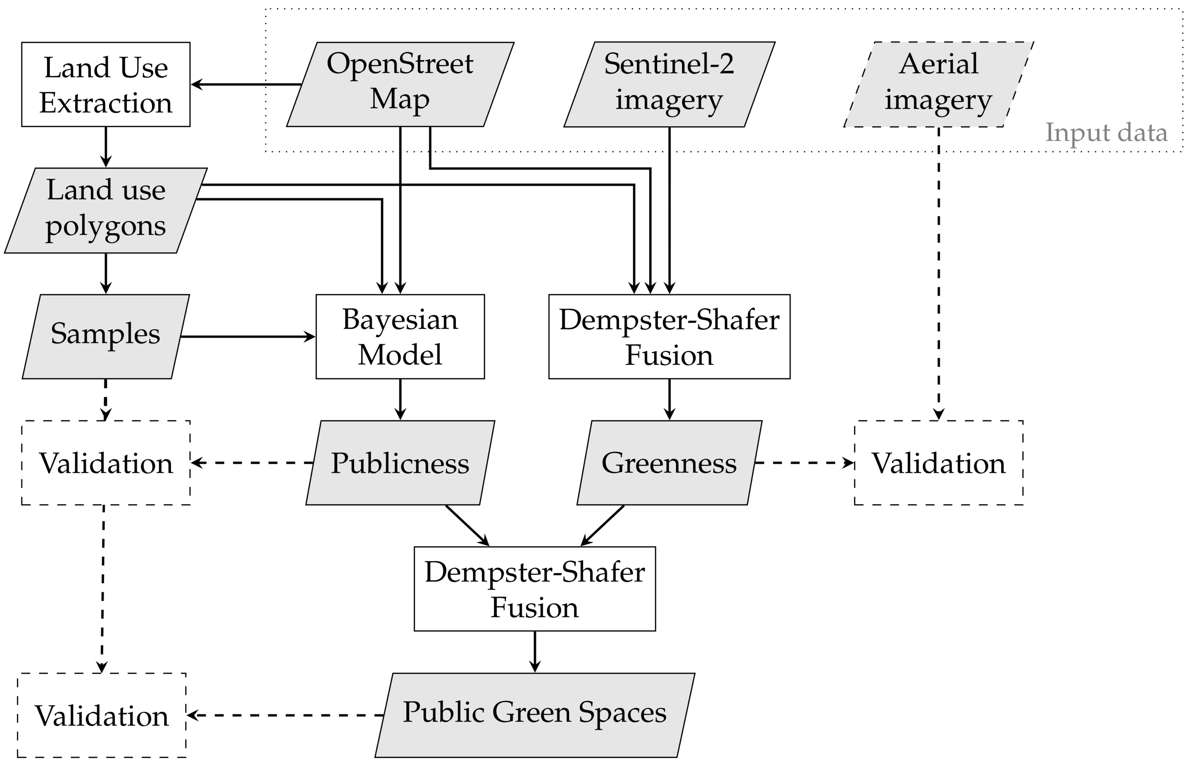
The conceptual framework of our methodology for mapping public urban green spaces consists of four parts (Figure 2). First, a mesh of homogeneous land use polygons was derived based on the OSM data (see Section 4.3.1). These polygons were the basis for all subsequent analyses. Public green spaces were characterized by their “greenness”, i.e., the presence of vegetation, and their “public accessibility” i.e., the accessibility by the general public. However, these characteristics are not equally well measurable using Sentinel-2 and OSM data, e.g., Sentinel-2 imagery is suitable to assess whether an area is vegetated, but not whether it is publicly accessible. Therefore, these two characteristics were modeled separately. The greenness was estimated by fusing information from Sentinel-2 imagery and OSM data using the Dempster–Shafer theory (see Section 4.3.2), while the public accessibility was modeled using a Bayesian logistic regression approach (see Section 4.3.3). In the last step, the modeled information on greenness and public accessibility were fused using the Dempster–Shafer theory to yield a map of public green spaces (see Section 4.3.4).
Validation was performed for the results of the greenness and public accessibility models as well as the final map of public urban green spaces. The aerial imagery was used to validate the results of the OSM and Sentinel-2 based greenness model. The public accessibility model was trained and validated using manually classified samples selected from the land use polygons (see Section 4.3.3). These samples were also used to evaluate the final map of public green spaces.
The whole analysis except for the generation of land use polygons was implemented in Python 3.7 [64]. PyMC3 [65] was used for Bayesian Modeling, and pyds [66] was used for Dempster–Shafer fusion. The generation of land use polygons was implemented using the software FME [67]. Data extraction was performed using the ohsome API [68] for OSM data and Google Earth Engine [69] for Sentinel-2 data. All data and Python source code can be found at [70].

4.3.1. Land Use Polygons

This section briefly describes the procedure for creating homogeneous land use polygons from OSM data, which were the basis for the subsequent mapping of urban green spaces. The main goal of this step was the generation of semantically meaningful polygon meshes in the context of public urban green spaces mapping. These polygons represent areas of homogeneous land use which form an independent activity space. They were delineated on the basis of assumptions about physical barriers resulting from the boundaries of certain neighboring land use class combinations extracted from OSM. The process of polygon generation essentially consisted of two steps: the city block generation process based on the traffic network and the further division of the blocks into sub-blocks based on land use information.
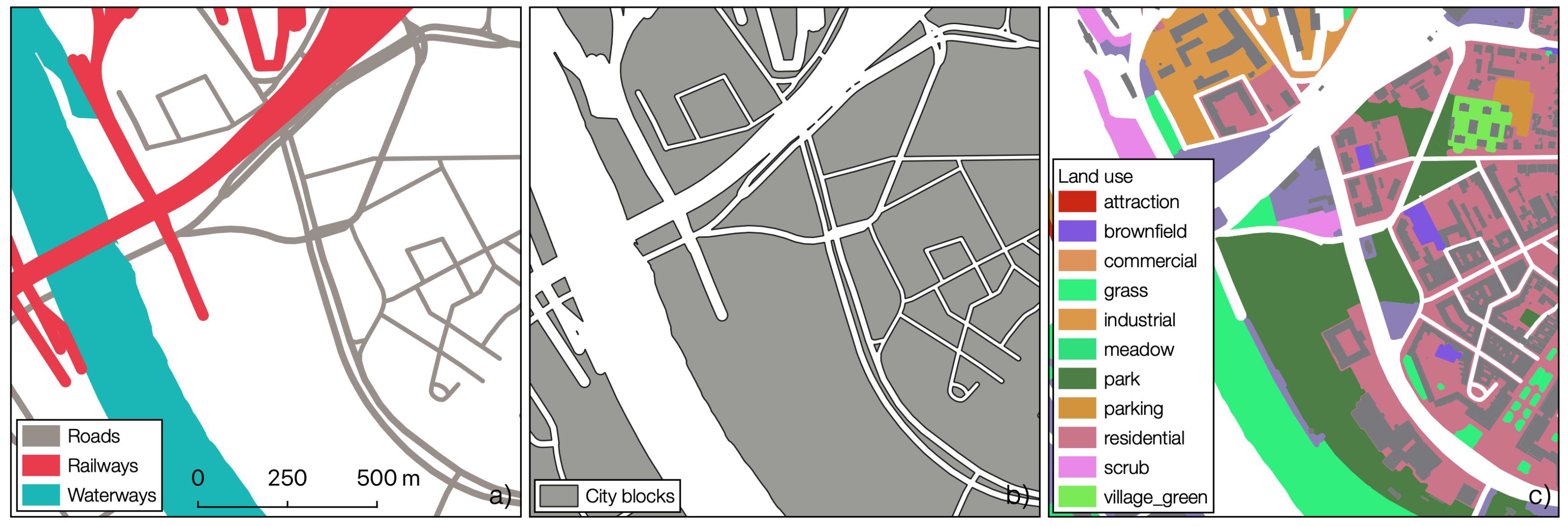
In the first step, city blocks, sometimes also referred to as street blocks, were generated using the network of roads, railway tracks and boundaries of large waterways (Figure 3a,b). We followed a similar approach as Grippa et al. [54] except that we also considered railways. Table 1 contains all OSM tags and geometry types, which were used to represent the traffic network. Line features were buffered with a width between 4 (e.g., living streets) and 10 m (e.g., railway tracks) depending on the type of the road. The waterway features were particularly necessary to ensure that the rivers banks of larger rivers or lakes were well represented in the city block map. All resulting features were intersected with each other to form the city blocks. To remove sliver polygons, all polygons less than 10 m in width were merged with the neighboring polygon using the criterion of the longest common edge.
In the second step, the city blocks were further divided into sub-blocks based on land use information derived from OSM (Figure 3c). A complete list of land use tags which were considered is given in the description of the basic probability assignment based on OSM in Section 4.3.2 Only OSM polygon features larger than 0.25 ha were included in this step. To dissolve polygons which contain the same land use but were mapped using different tags (e.g., landuse=forest and natural=wood both represent forest) OSM tags were grouped into land use classes using a rule-based approach. This aggregation was however only done for the generation of the geometries. The original land use tag of the resulting polygons was preserved in the attribute table. In case several land use related tags were present within one polygon, the tag with the highest area fraction was used.
The intersection between the city blocks and the land use data followed certain rules when multiple polygons were overlapping, e.g., a leisure=park feature located inside a landuse=residential feature. In this case, the smaller feature contained in the larger one was given priority to get an overlap-free sub-block geometry. However, when the two land use polygons could be seen to form a common green space entity (e.g., a leisure=playground polygon within a landuse=grass polygon), then the polygons were merged in an automated way based on predefined rules. If a smaller polygon partially overlapped another one, then the smaller polygon was split in two parts unless it contained a green space related tag such as leisure=park. In this case, the polygon remained unchanged and was given priority over the other one. If an OSM feature had an additional access=* tag, it was assigned to the respective land use polygon. As a final step, the building features from OSM were intersected with the land use polygon mesh.

4.3.2. Greenness Model

The greenness of each land use polygon was derived from OSM data and Sentinel-2 satellite imagery and subsequently fused using the Dempster–Shafer theory. Since these sources can be considered as independent, Dempsters’s combination rule was used. The frame of discernment for this data fusion task is defined as θ g = { g r e e n , g r e y } , i.e., an object can be vegetated or non-vegetated.
To quantify the amount of vegetation from aerial or satellite imagery, the Normalized Difference Vegetation Index (NDVI) is frequently used [21]. It is calculated using
N D V I = N I R R E D N I R + R E D
where N I R and R E D represent the reflectance at the near-infrared and red bands.
Bands 4 and 8 of the Sentinel-2 imagery were used to calculate the NDVI with a resolution of 10 m. To capture the annual peak in vegetation presence at each location from the Sentinel-2 imagery, a maximum NDVI image composite was created using Google Earth Engine. In a maximum NDVI composite, several satellite scenes are fused into one image by selecting the highest NDVI value of each pixel to generate a homogeneous, cloud free image composite. All Sentinel-2 scenes captured within 2019 which had a cloud coverage of less than 5% were selected. This yielded 40 scenes captured between 22 January 2019 and 11 October 2019, which were used to create the image mosaic.

Basic Probability Assignment Based on Sentinel-2

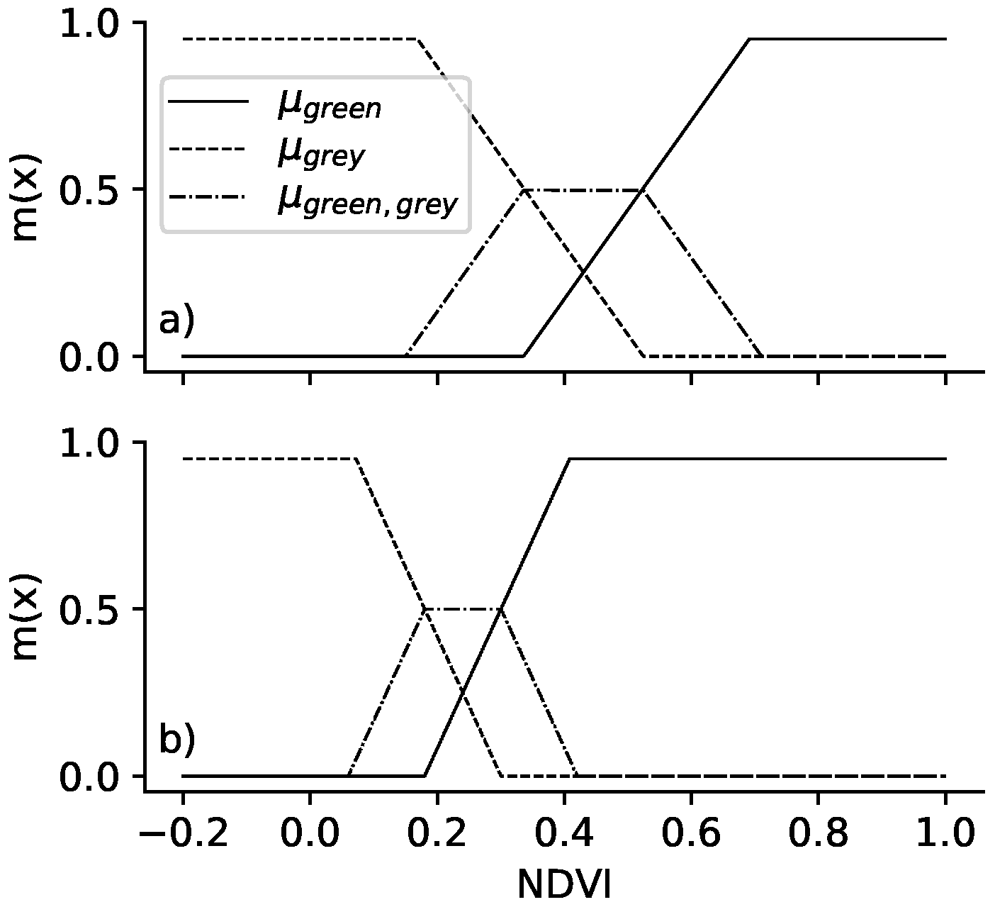
There is a linear relationship between the NDVI and the presence of vegetation with high NDVI values indicating high amounts of healthy vegetation [71]. Therefore, the belief about whether an area is vegetated (green) or non-vegetated (grey) can be quantified based on the NDVI value. For the basic probability assignment, three functions were set up to map NDVI values to the probability masses m ( { g r e e n } ) , m ( { g r e y } ) and m ( { g r e e n , g r e y } ) (Figure 4a). The last one represents the uncertainty due to mixed pixels in the imagery which cover both vegetated and non-vegetated areas.
Equation (8) exemplifies how the probability mass m ( { g r e e n } ) was calculated. NDVI values higher than h g r e e n and lower than h g r e y indicate g r e e n or g r e y areas with a high degree of certainty, i.e., m ( { g r e e n } ) = 0.95 . The maximum probability mass was set to 0.95 instead of 1.0, so that the Dempster–Shafer fusion does not yield counter-intuitive results. NDVI values close to h m i x e d were assigned probability masses m ( { g r e e n } ) = 0.25 , m ( { g r e y } ) = 0.25 and m ( { g r e e n , g r e y } ) = 0.5 . This represents the belief that these pixels must be at least partly vegetated and non-vegetated but with a high degree of uncertainty about the exact ratio. The shift value s was chosen so that m ( { g r e e n , g r e y } ) = 0.5 at h m i x e d .
m g r e e n = 0 if NDVI h m i x e d s 0 0.95 if h m i x e d s < NDVI < h g r e e n 0.95 if NDVI h g r e e n
where h g r e e n is the NDVI value representative for vegetated area, h m i x e d is the NDVI value representative for mixed land cover, and s is a shift value, which needs to be defined so that m ( { g r e e n , g r e y } ) = 0.5 at h m i x e d .
To find representative NDVI values for vegetated, non-vegetated and mixed land cover areas, unsupervised clustering with three cluster centers was applied sparately to the NDVI images derived from the aerial and satellite image. Both regular K-means clustering [72] and fuzzy C-means clustering [73] were tested. In contrast to regular clustering methods, fuzzy C-means clustering is based on fuzzy sets instead of crisp categories thereby considering the inherent uncertainty in the class assignment. Fuzzy C-means clustering yielded cluster centers which better represented the vegetated, non-vegetated and mixed class, which is why results of this method were chosen for the basic probability assignment (Table 2).
The basic probability assignment for a land use polygon was derived by applying the functions in Figure 4 to the NDVI values of the pixels intersecting the respective polygon. The resulting values were aggregated using the mean to yield the probability masses m o s m ( g r e e n ) , m o s m ( g r e y ) and m o s m ( g r e e n , g r e y ) for each polygon. This approach yielded good greenness estimates for polygons larger than the 10 m pixel size of the Sentinel-2 imagery because they did not contain any mixed land use pixels. However, within urban environments, the 10 m resolution is not sufficient to accurately capture small land use objects such as little huts or small land use patches. This was reflected in highly uncertain greenness estimates for these objects.

Basic Probability Assignment Based on OSM

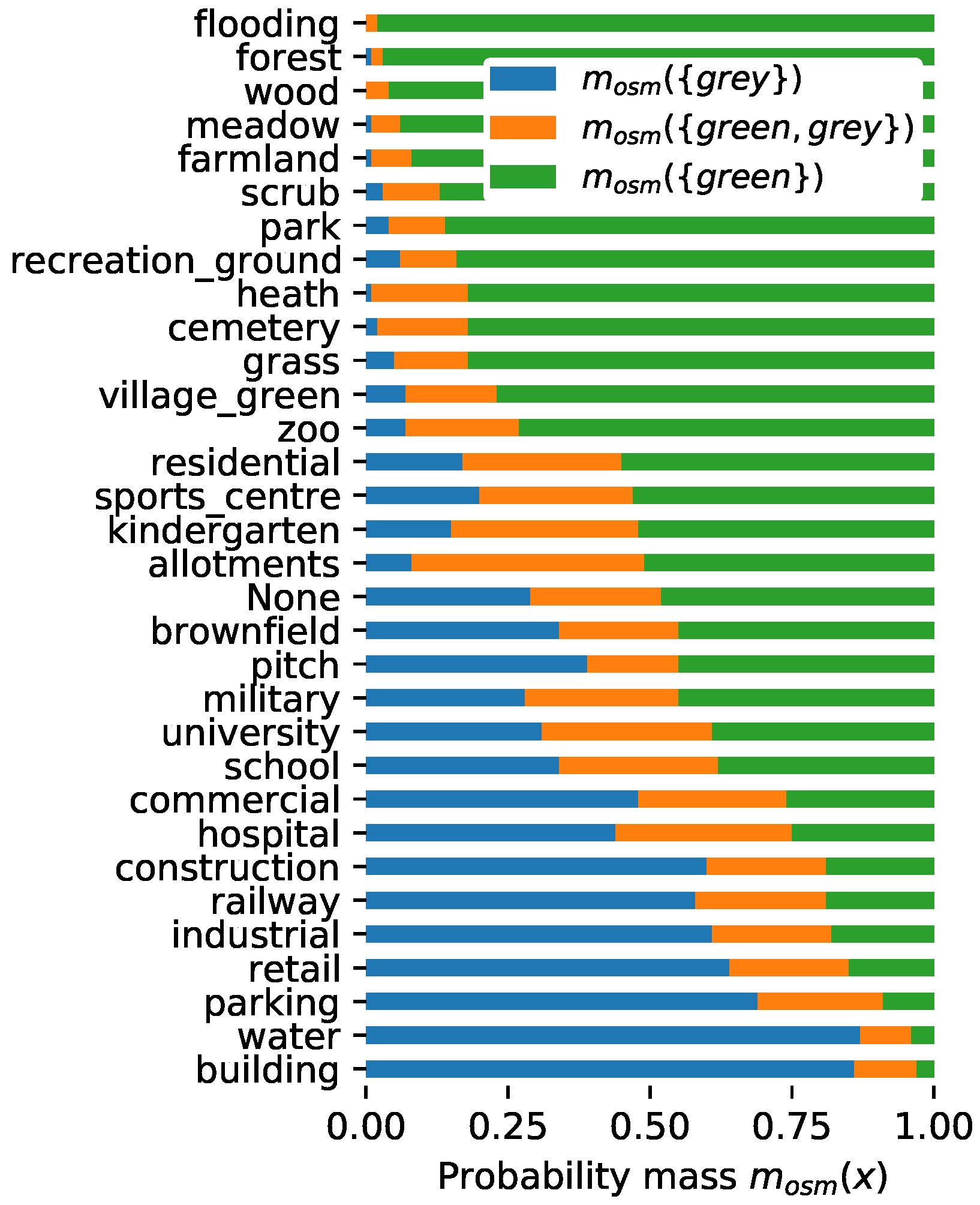
To alleviate the problem of insufficient spatial resolution of the Sentinel-2 imagery, OSM data was used to improve the greenness estimates. Certain OSM tags are more associated with greenness than others, e.g., an object with the tag leisure=park is more likely to contain vegetation than an object with the tag building=*. Still, this association is not the same everywhere due to climatic and cultural factors [74]. Instead of compiling a static list of OSM tags which are to be considered as green based on expert knowledge, the belief in the greenness associated with each OSM tag was derived from Sentinel-2 data. This was done by extracting only NDVI pixels which were fully located inside objects with the respective tag. In this way, the uncertainty due to mixed pixels on the edges of the objects was excluded. The basic probability assignment of the Sentinel-2 data (Figure 4a) was applied to all NDVI values belonging to an OSM tag. The resulting values were aggregated using the mean to yield the probability masses m o s m ( g r e e n ) , m o s m ( g r e y ) and m o s m ( g r e e n , g r e y ) for each OSM tag (Figure 5).
An example to demonstrate the process will be described as follows: Let us assume there are two pixels p 1 and p 2 which belong to the same OSM land use class t. Their NDVI values are 0.5 and 0.65. Applying the probability mass assignment shown in Figure 4 to these NDVI values yields m p 1 ( g r e e n ) = 0.44 , m p 1 ( g r e y ) = 0.06 and m p 1 ( g r e e n , g r e y ) = 0.5 and m p 2 ( g r e e n ) = 0.84 , m p 2 ( g r e y ) = 0 and m p 2 ( g r e e n , g r e y ) = 0.16 , respectively. Calculating the mean of these probabilities yields m o s m ( g r e e n ) = 0.64 , m o s m ( g r e y ) = 0.03 and m o s m ( g r e e n , g r e y ) = 0.33 as probability mass for the tag t.
OSM tags describing vegetated areas such as landuse=forest or leisure=park showed high probability mass values for m ( g r e e n ) , while built-up areas such as buildings or parking lots showed high probability mass values for m ( g r e y ) . The basic probability assignment for buildings did not contain much uncertainty, since mixed pixels (i.e., due to small buildings) were not considered for the derivation of the OSM based probability masses. The basic probability assignment for the tag landuse=allotments showed the highest value in m ( g r e e n , g r e y ) and therefore the highest uncertainty, since the little huts located inside these community gardens were not mapped in OSM leading to many mixed pixels in these areas.

Validation

The accuracy of the greenness derived from Sentinel-2 only and from the combination of Sentinel-2 and OSM was evaluated by comparing them to the greenness derived from the higher resolution aerial image (see Section 4.2). First, the aerial image was resampled using nearest neighbor resampling to a resolution of 1 m which was sufficient for this validation and saved processing resources. Subsequently the NDVI was calculated and fuzzy C-means clustering was used to adjust the functions of the basic probability assignment to the spectral characteristics of the aerial imagery (Figure 4b, Table 2). The Root Mean Square Error (RMSE) between the probability masses derived from the aerial imagery and the Sentinel-2 and OSM data was calculated to evaluate the potential of OSM to compensate for the insufficient spatial resolution of Sentinel-2. In addition, three greenness maps containing the classes green and grey were created based on the different data sets (aerial imagery, Sentinel-2 and Sentinel-2 + OSM) by assigning the class with the highest pignistic probability to each land use polygon. If the pignistic probability was at 0.5, the object was classified as uncertain.

4.3.3. Public Accessibility Model

The aim of the public accessibility model was to distinguish public from private green spaces. Public access means in this context that an area is freely accessible for the general public without prior permission. It does not imply assumptions about the ownership of the area. Apart from municipal green spaces such as parks this definition also includes privately owned areas which are accessible for the general public e.g., playgrounds which belong to apartment blocks. The two target classes of the model were public and private.

Indicators in OSM for Predicting Public Accessibility

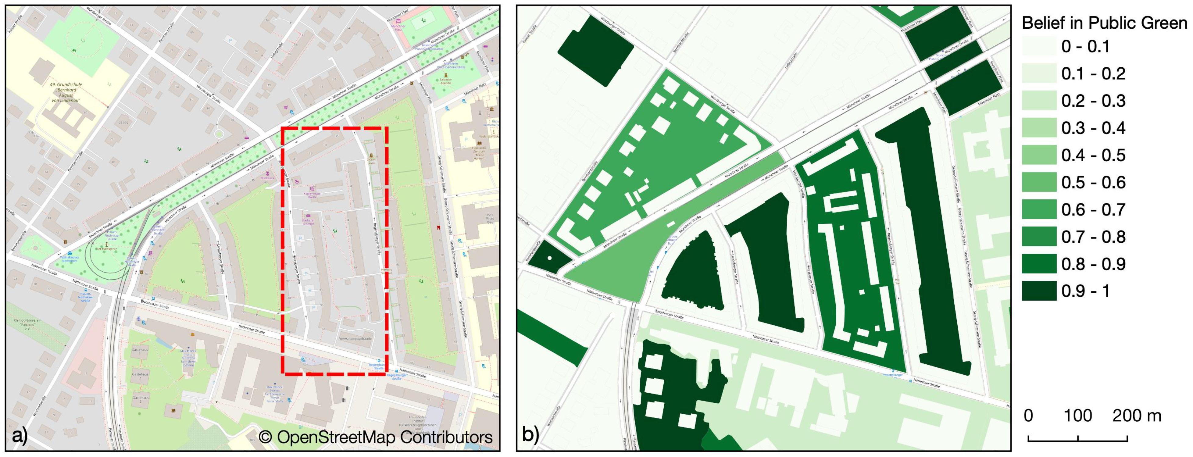
Since satellite imagery does not always yield reliable information about the land use of an area, only OSM data was used to distinguish public from private green spaces. In contrast to private green spaces (e.g., residential gardens) public green spaces are usually well represented in OSM and are being mapped using different tags such as leisure=park, landuse=grass or landuse=village_green. OSM features with these tags can be assumed to be publicly accessible unless one of the tags access=no or access=private are given as well. Still, the mapping practice in regard to public green spaces in OSM is not always consistent leading to spatially heterogeneous levels of completeness. Out of the four public green spaces only three have been mapped as landuse=grass. Still, the unmapped public green space in the middle can be recognized as such using contextual information such as the presence of a path network or green spaces specific POIs (e.g., playground). For the region of Dresden, paths as well as benches and playgrounds are very often mapped within public green spaces in OSM making them good contextual indicators for identifying unmapped public green spaces in OSM. This was explored in a previous study by performing association rule mining on parks mapped in OSM within different cities in the world [75]. Based on these results, the features listed in Table 3 were considered for distinguishing public from private green spaces.
Considering the presence of benches or playgrounds as binary variables instead of the absolute number of benches or playgrounds within the polygon leads to better model fit and better convergence of the models. To enable better sampling during model fitting, the path length and density as well as the number and density of intersections were transformed to be more normally distributed using the Yeo Johnson transformation [76].

Model Structure

A Bayesian hierarchical logistic regression approach was used to model the public accessibility, because all indicators were linearly related to public accessibility and a hierarchical approach seemed suitable to represent the different land use categories. During model evaluation different model configurations were compared: A pooled model which only considered the contextual indicators, but not the information on land use and a multi-level approach with a partially pooled intercept α j [ i ] which represented the land use categories j. All land use specific intercepts originated from a common normal distribution with mean μ α and standard deviation σ α 2 . The complete multi-level model including the contextual indicators was defined as
p ( y i = 1 ) = 1 1 + e ( α j [ i ] + β X i )
with
α j [ i ] N ( μ α , σ α 2 )
where p ( y i = 1 ) is the probability that the polygon i is public, α j [ i ] is the partially pooled intercept for each land use class j, X is the vector of contextual indicators and β the vector containing the coefficients for the contextual indicators.
Little prior knowledge existed about the values of the model parameters. Therefore, the priors for the model were chosen to be weakly informative but within reasonable parameter spaces. The sensitivity of the model towards different priors was evaluated to ensure model convergence and reasonable model results. Since the context variables were standardized and therefore share the same scale, the priors of all coefficients were chosen to be weakly informative normal distributions as suggested by Lemoine [77] with mean μ = 0 and standard deviation σ = 10 . To allow for sufficient variance between the intercepts representing the different land use tags, the prior of the multi-level intercept μ α was also set up as a weakly informative normal distribution whose mean was defined as a normal distribution with μ = 0 and σ = 10 and whose standard deviation σ α was defined as a Half Cauchy distribution as suggested by Polson et al. [78] and Lemoine [77]. The scale parameter of the Half Cauchy distribution was set to β = 5 . The model was trained with 3 chains and 10,000 iterations.

Model Training and Validation

For the training and validation of the model, 300 land use polygons were selected using a stratified random sampling approach based on the land use types of the polygons (see Section 4.3.1). These were manually classified as public or private green spaces based on aerial imagery and Google Street View [79]. Seventy percent of samples were used for model training, the remaining 30% for testing. Model comparison was performed using the leave-one-out cross validation (LOO) criterion [80]. Since the logarithm of L O O l o g ( L O O ) was used, higher values indicate higher model quality.

Conversion of Posterior Probabilities to Probability Masses

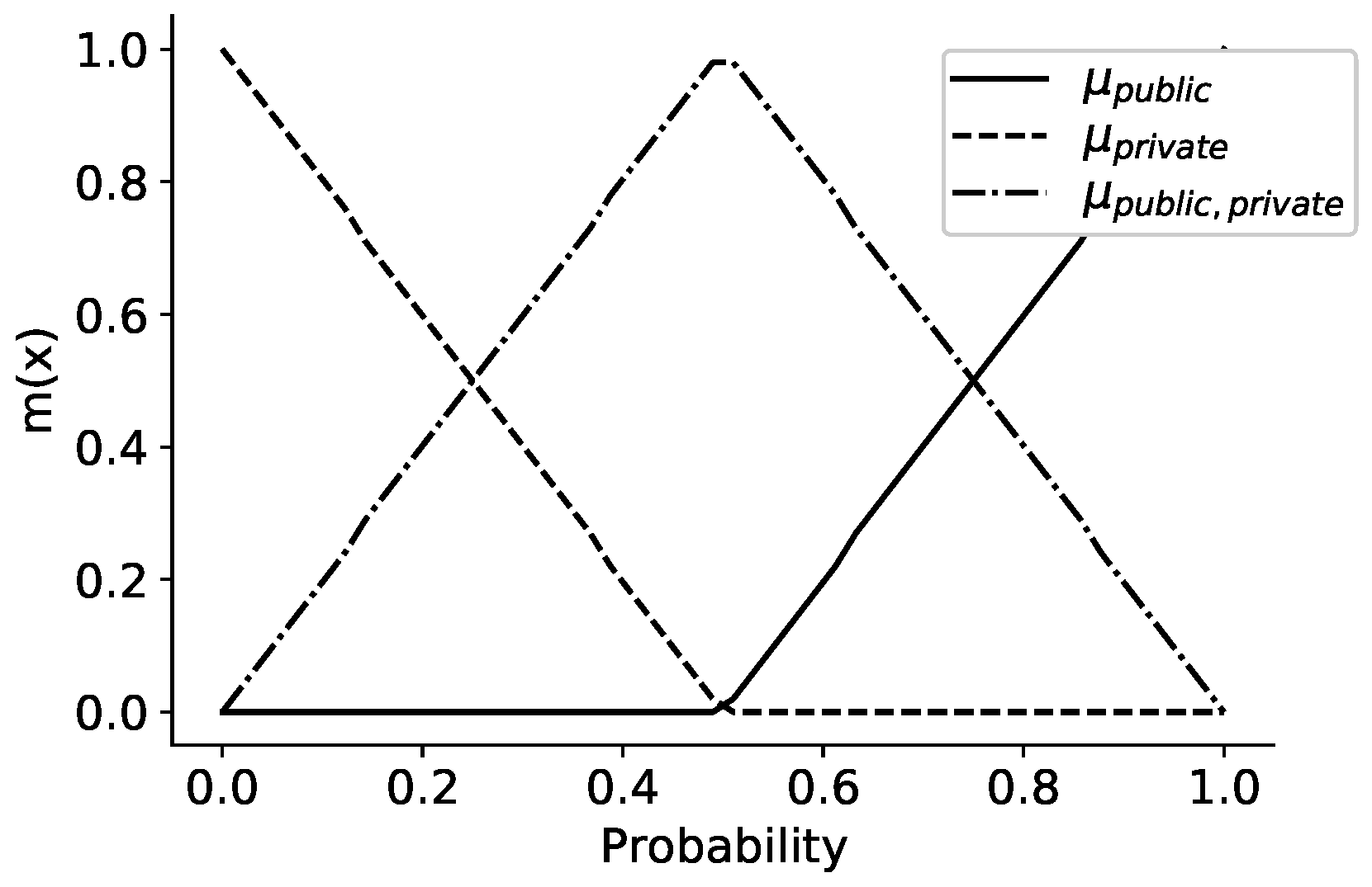
In order to fuse the model results on public accessibility with the belief in greenness (see Section 4.3.2) the posterior probabilities of the Bayesian model had to be converted to beliefs expressed as probability masses. The frame of discernment of this basic probability assignment was θ p = { p u b l i c , p r i v a t e } . The basic probability assignment is based on the functions shown in Figure 6. Highest certainty in class assignment was given when the model probability was p ( y i = 1 ) = 0 or p ( y i = 1 ) = 1 . Probability values contain increasingly more uncertainty as they approach a value of 0.5. At this point, uncertainty in class assignment is highest, so m ( { p u b l i c , p r i v a t e } ) is at its maximum. The functions of the basic probability mass assignment were applied to all posterior probabilities and the resulting values were aggregated using the mean to derive scalar values for m ( { p u b l i c } ) , m ( { p r i v a t e } ) and m ( { p u b l i c , p r i v a t e } ) .

4.3.4. Fusion of Greenness and Public Accessibility

In the final step, the derived beliefs on greenness and public accessibility were fused using Dempster’s rule of combination to produce a map of public urban green spaces. The greenness and public accessibility were represented using two different frames of discernment θ g = { g r e e n , g r e y } and θ p = { p u b l i c , p r i v a t e } . Since the greenness and public accessibility were modeled separately, they can be seen as independent of each other. Therefore, the combination of these two frames of discernment was achieved by building the Cartesian product of them which yielded the new joint frame of discernment θ p g
θ p g = θ p × θ g = { ( g r e e n , p u b l i c ) , ( g r e e n , p r i v a t e ) , ( g r e y , p u b l i c ) , ( g r e y , p r i v a t e ) }
For the final fusion, the probability masses of the two models were converted to the new frame of discernment θ p g using
m ( { ( g r e e n , p r i v a t e ) , ( g r e e n , p u b l i c ) } ) = m ( { g r e e n } )
m ( { ( g r e y , p r i v a t e ) , ( g r e y , p u b l i c ) } ) = m ( { g r e y } )
m ( { ( g r e e n , p u b l i c ) , ( g r e y , p u b l i c ) } ) = m ( { p u b l i c } )
m ( { ( g r e e n , p r i v a t e ) , ( g r e y , p r i v a t e ) } ) = m ( { p r i v a t e } )
An example should demonstrate the principle of the conversion: the belief about the greenness of a land use polygon does not contain any information about its public accessibility. Therefore, the probability mass m ( { g r e e n } ) of the frame of discernment θ g is assigned to the union of the elements (green, public) and (green, private) in the new frame of discernment θ , because based on this belief it could be either of the two.
After the beliefs on greenness and public accessibility were fused, the pignistic probabilities were calculated and the class with the highest pignistic probability was assigned to each object e.g., (public,green), (public,grey), (private,green) or (private,grey). Selecting all objects classified as (public,green) yielded the final map of public green spaces.
The uncertainty in regard to the probability that an object represents a public green space was quantified by calculating the difference between the plausibility and the belief of the set {(public,green)}
u ( { ( p u b l i c , g r e e n ) } ) = p l ( { p u b l i c , g r e e n } ) b e l ( { p u b l i c , g r e e n } )
The uncertainty associated with the information on public accessibility or greenness was calculated in the same way but based on the sets {(public,green), (public,grey)} and {(public,green), (private,green)}.

4.3.5. Validation

The public green space map was validated using 300 samples extracted from the land use polygons (see Section 4.3.3). They were manually classified into the classes public green space or other using aerial imagery and Google Street View [79]. Based on this validation data, an accuracy assessment was conducted which included the measures precision, recall and the f1 score [81].

5. Results

5.1. Land Use Polygons

Within the study area 3776 land use polygons were created out of which 83.8% were tagged as buildings, 5.2% as landuse=residential, 2.1% as landuse=grass and 0.8% as leisure=park. 2.7% of polygons did not contain any land use related OSM tag. The remaining land use categories constituted less than 0.5% each. 8.4% of the non-building polygons contained at least one playground, 8.7% contained at least one bench and 29.3% of polygons contained at least one footpath intersection. Restricted access, indicated through the presence of one of the tags access=no|private|customers, was given for only 2% of non-building polygons.

5.2. Greenness

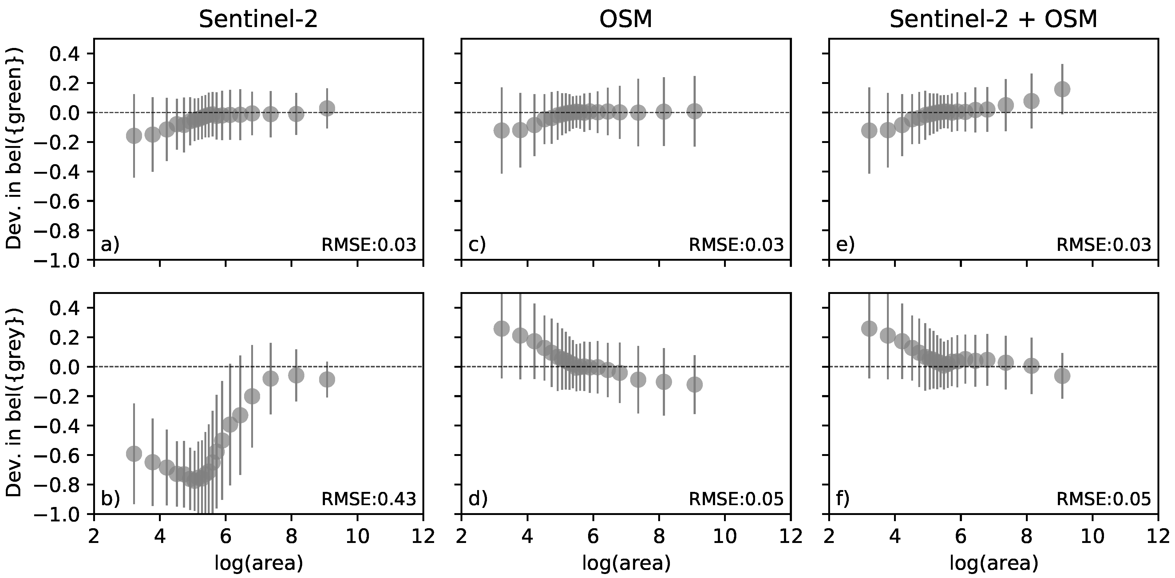
The beliefs about greenness based on Sentinel-2 and OSM data were compared to the belief derived from the aerial image as reference data (Figure 7). The beliefs derived from Sentinel-2 imagery were less accurate than the ones derived from the combination of Sentinel-2 and OSM data. The RMSE of the probability masses m ( { g r e y } ) derived from Sentinel-2 data was at 0.43 with highest deviations among polygons smaller than 500 m 2 which is due to the fact that the sensor resolution is not high enough to capture their greenness accurately (Figure 7b). These objects are mostly buildings which are mapped with a very high completeness in OSM. Fusing the evidence from Sentinel-2 and OSM led to a strong improvement of the greenness with the RMSE dropping to 0.05 (Figure 7f). After the fusion, the probability mass m ( { g r e y } ) of very small buildings such as huts was overestimated compared to the reference data, which can be explained by the fact that these huts were often covered by trees and therefore appeared vegetated in the aerial imagery (Figure 7d,f).
These differences could also be seen in the classifications derived from the beliefs (Figure 8). When using Sentinel-2 imagery only, most of the small buildings could not be reliably classified as green or grey but remained uncertain due to the high uncertainty cause by the mixed pixels (Figure 8a). The belief derived from OSM on the greenness of objects with the tag building=* however was very clear as m ( g r e y ) 0.8 (Figure 5b)). So fusing the Sentinel-2 based belief with evidence from OSM increased the number of buildings being correctly classified as grey considerably (Figure 8b).
Regarding the deviance in probability mass m ( { g r e e n } ) , the overall RMSE remained at 0.03 even after the fusion with the OSM data (Figure 7a,e). Some deviations occurred within areas with dynamically changing land cover such as construction sites or agricultural areas (e.g., farmland, grassland or meadow). These deviations were probably due to actual land use changes which have taken place between the acquisition dates of the aerial image in 2017 and the Sentinel-2 imagery in 2019. Still, fusing evidence from OSM with Sentinel-2 imagery led to improvements in the detection of green areas. Especially small green spaces which are often mapped in OSM using the tag landuse=grass were detected more reliably. Among land use polygons smaller than 500 m 2 (excluding buildings) the overall accuracy increased from 0.18 using Sentinel-2 only to 0.48 using Sentinel-2 and OSM data. Of these small polygons, 72% contained an OSM tag such as landuse=grass (28%), landuse=residential (16%) or amenity=playground (7%).

5.3. Public Accessibility

The most basic multi-level model which only considered the land use tags ( l o g ( L O O ) = −63, overall accuracy = 0.88) performed significantly better than the best pooled model which only considered the context indicators ( l o g ( L O O ) = −117, overall accuracy = 0.74). This indicates that the land use information in OSM was very important for the model to distinguishing public from private green spaces. OSM tags such as leisure=park or landuse=cemetery had positive intercepts suggesting that they were strong indicators for public green spaces, while OSM tags such as landuse=industrial or amenity=parking were indicating the opposite (Figure 9a). For residential areas or polygons without a land use tag, the intercepts were slightly negative, suggesting that these areas were only classified as public if the contextual indicators for public accessibility were strong enough.
To analyze the model’s potential to detect unmapped public green spaces, the influence of different context indicators on the model performance was investigated (Figure 9b). The multi-level model which only considered the land use related tags but no context indicators reached an overall accuracy of 0.88. Recall for class public was only at 0.77, since unmapped public green spaces were falsely classified as private.
Including the density of footpath intersections in the model slightly increased the overall accuracy to 0.90. The number of omission errors decreased, since some of the unmapped public green spaces could be detected using the additional footpath intersections. However, at the same time, the number of commission errors increased as a few private residential blocks containing footpaths along streets or access paths to single family houses were falsely classified as public. Although including the density of footpath intersections in the model was not sufficient to reliably detect all unmapped public green spaces, the uncertainty associated with the predictions of the samples m ( { p u b l i c , p r i v a t e } ) decreased by 22% on average compared to the multi-level model that did not consider the density of footpath intersections.
Generally, using the density instead of the absolute number of intersections per polygon led to a better model performance (Figure 9b), but using footpath intersections instead of overall footpath length performed only marginally better. Since the computation of the intersections is more computationally intensive, using the footpath length instead of the footpath intersections would be acceptable for the sake of saving computational resources if the model is to be applied to larger regions.
Adding the presence of benches and playgrounds as typical indicators for public green spaces in Dresden to the multi-level model further increased the overall accuracy to 0.98. The uncertainty associated with the predictions m ( { p u b l i c , p r i v a t e } ) decreased by 33% on average compared to the multi-level model without any context indicators. Precision and recall of the model were very high as well indicating that the model was able to detect most unmapped public green spaces without falsely classifying private residential areas (Table 4). Still, one omission error occurred for a polygon which did not contain any land use tag or context indicator. One commission error occurred for a land use polygon tagged as landuse=grass and access=private. This classification error could not be avoided even after including the access=* tag in the model. The tag landuse=grass is a strong indicator for public accessibility, but the influence of the tag access=private in the model was very low. This indicates that the model did not accurately capture the fact that the access=private tag implies no public accessibility with a high degree of confidence, which is likely due to the fact that the access=* tag was only given for about 2% of the land use polygons.

5.4. Fusion of Greenness and Public Accessibility

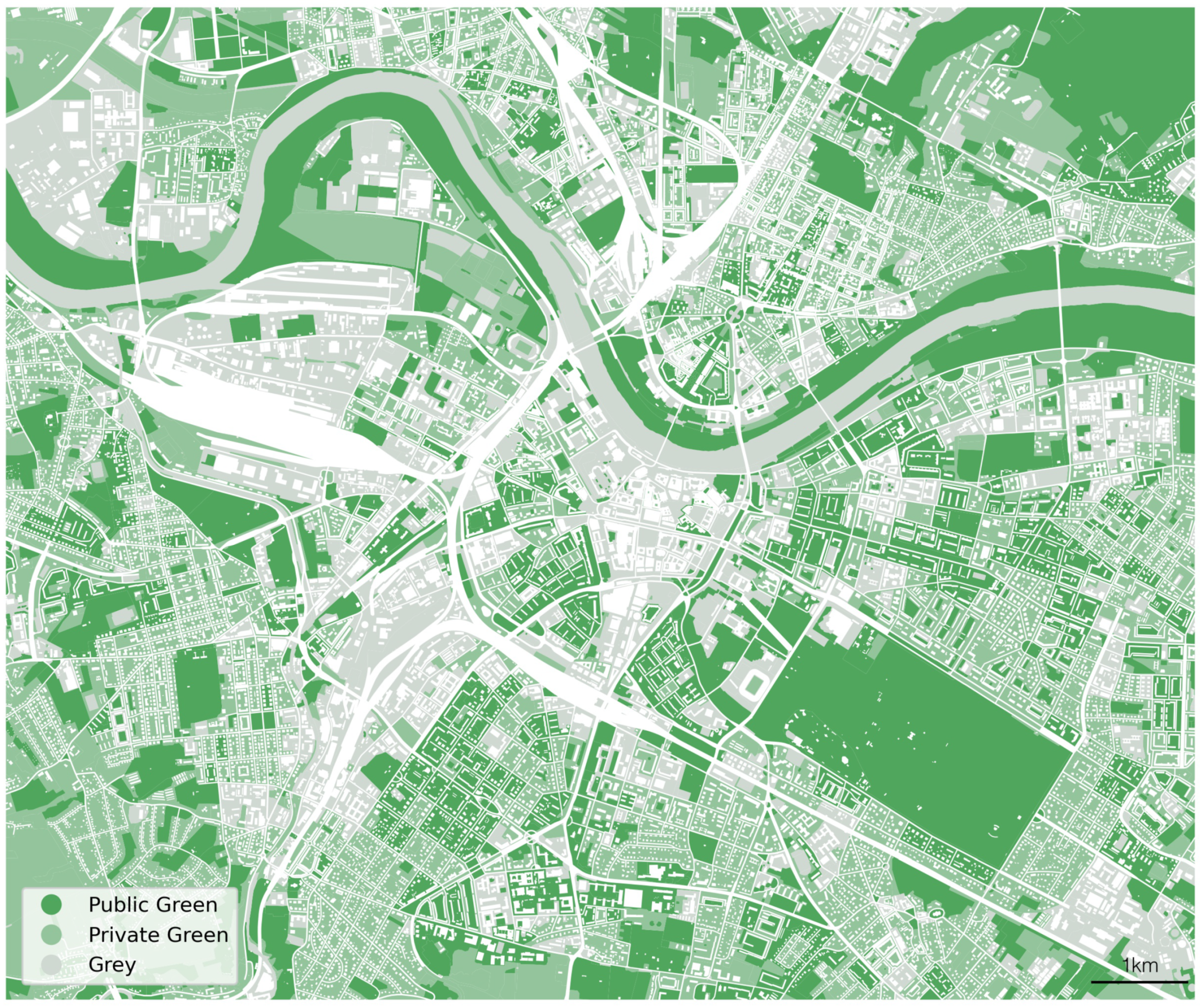
A map of public and private urban green spaces based on Sentinel-2 and OSM data is presented in Figure 10. Compared to the authoritative data on public green spaces shown in Figure 1), our prediction indicated the presence of a lot more green spaces. This is due to the fact that the former map does not contain privately owned but publicly accessible green spaces, since these were not included in the municipal data.
Overall accuracy of the final map of public green spaces was at 95%. Public green spaces which were mapped in OSM as leisure=park or landuse=grass were all reliably detected by the model. Among them are most municipal green spaces, which were mapped in Dresden with a high level of completeness as well as some privately owned but publicly accessible green spaces. Public green spaces which have not been mapped in OSM explicitly using these tags were also detected by model with slightly weaker beliefs (Figure 11b). Within the whole study area, 180 of such presumably unmapped public green spaces were detected, most of them within residential areas. Green spaces which were tagged as private using the access=* were partly misclassified by the model as public.
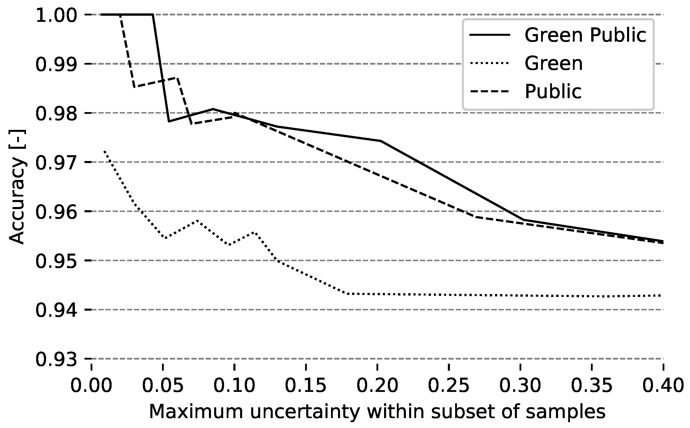
Figure 12 shows the relationship between the uncertainties of the predictions and the overall model accuracy. With the level of maximum uncertainty in the subsets of samples rising, the model accuracy was decreasing. This indicates a linear relationship between the model accuracy and the uncertainty estimate of the samples. The same pattern was visible for the uncertainty of the public accessibility belief indicating that the overall uncertainty in the model predictions was mainly driven by the uncertainty of the public accessibility model. The uncertainty in greenness on the other hand did not show such a strong relationship with the overall model accuracy suggesting that the uncertainty in greenness did not influence the model accuracy as much.

6. Discussion

The aim of this study was to develop and test a methodology to alleviate current limitations in urban green space mapping due to the uncertainties inherent in the Sentinel-2 and OSM data. A common problem of using Sentinel-2 imagery for urban green space mapping is its inability to capture small objects due to its insufficient spatial resolution (RQ1). This was confirmed in this study, but it was also shown that OSM data can partly compensate for these inabilities. Especially among small land use objects such as buildings or green spaces smaller than 500 m 2 , the detection rate was increased significantly by considering the data source specific uncertainties during the data fusion using the Dempster–Shafer theory.
Another limitation of satellite data in regard to urban green space mapping is the inability to distinguish public from private green spaces (RQ2). OSM data was proven to be suitable to compensate for this problem as well using a Bayesian logistic regression model. To account for the inconsistent and incomplete representation of public green spaces in OSM, land use specific OSM tags as well as contextual indicators for public accessibility (e.g., footpaths) were considered in the model. In this way, it was possible to detect both explicitly mapped public green spaces as well as public green spaces which are missing in OSM. Still, the model can be improved, for example, by a more accurate recognition of restricted accessibility indicated by the access=* tag. Although the meaning of this tag is very clear, its influence was quite small in the model, because it occurs in only 2% of the samples. To increase its influence, the access=* tag could be excluded from the model and instead be treated as an independent information source and converted to a probability mass to be fused with the model results. In this context, it would also be interesting to analyze how conditional accessibility, e.g., areas with access fees or time dependent access restrictions on school grounds, could be derived from OSM data.
Modeling the greenness and public accessibility separately and fusing them in the final step using the Dempster–Shafer theory made it possible to propagate the uncertainties from the data sources through the analysis up until the final map of public green spaces (RQ3). The uncertainty regarding the evidence for public access had a higher influence on the model accuracy than the evidence for greenness. This information allowed a better understanding of the reliability of the final map of green spaces and might help in reducing the amount of manual validation work need to make the data set reliable enough to be used within a recommendation system.
Since Sentinel-2 imagery and OSM data are available globally and free of charge, the methodology is in principle also applicable to other cities or regions. The greenness model can be applied automatically to other areas without manual interventions and due to the high-revisiting rate of the Sentinel-2 satellites the production of cloud free image composites is usually possible for most areas of the world.
However, it is very important to stress that the quality of final public green space map is highly dependent on the quality of the underlying OSM data. Within our study area, the completeness of the OSM data in regard to buildings, public green spaces and the contextual indicators for public accessibility was very high which allowed for reliable high quality results [75], but this should not be assumed for other geographic areas without prior data quality analyses of the local OSM data. An analysis of completeness of relevant OSM features based on intrinsic data quality indicators [82] could be the first step before undertaking the next steps. The OSHDB and the ohsome API [68] might serve as entry points for such an analysis.
Although a comprehensive analysis of the transferability of the method to other cities was outside the scope of this paper, successfully applying the method to other cities is likely possible if the OSM data quality is sufficient and the public accessibility model is adapted to the local OSM data. Predicting public accessibility based on the land use tags and the density of footpath intersections already yielded good results with an overall accuracy of 0.9. Since the meaning of these OSM objects in regard to the presence of public green spaces can be assumed to be fairly similar across geographical regions, this model should yield comparable results when trained and applied to other cities with similar levels of completeness. Still, the inclusion of region specific context indicators which are typical for public green spaces in the respective city is important to reliably capture unmapped public green spaces as well. In the case of Dresden, benches and playgrounds were important local context indicators, but in other regions different OSM tags might have to be used, since characteristic elements of public green spaces vary depending on the local culture and the mapping practices in OSM [74]. Therefore, it is very important to identify suitable context indicators which are both culturally relevant in regard to local public green spaces and are mapped with a sufficient level of completeness within OSM when transferring the model to other areas. Data-driven feature selection techniques such as association rule mining can be used to assist in finding suitable indicators [75].
There is potential to improve the proposed method by considering additional data. Point or line objects in OSM such as trees or tree rows were not considered in this study, but if considered in addition, they could presumably further improve the greenness estimates. In the same way, including physical barriers such as walls or fences mapped in OSM could improve the generation of land use polygons. Social media data could be used as an additional source of evidence to improve the predicted public accessibility.
An important question for future studies is to what extent the maps of public green spaces created using this methodology are comparable between different cities. Are all kinds of green spaces captured or is there a bias towards capturing certain kinds of green spaces in some cities but not in others depending on the selection of contextual indicators for public accessibility? To what extent are these biases influenced by the OSM data quality, the mapping practices of the local OSM community and the region specific characteristics of urban green spaces? These potential problems should be analyzed and if necessary addressed by developing suitable methods to guarantee the production of consistent maps of public urban green spaces across multiple cities. This would be an important step towards facilitating accessibility analyses on urban green spaces across different cities [11,83] for which suitable data sets are not available yet. In addition, the urban green spaces derived using this methodology could also be of interest for the OSM community by raising awareness for a lack of completeness or inconsistent mapping practices in regard to urban green spaces.

7. Conclusions

Our results showed that fusing OSM and Sentinel-2 data based on Dempster–Shafer theory improved estimates of public urban green spaces to a remarkable degree. This offers potential for improved assessments of urban green spaces and their attached ecosystem services—at least in regions of sufficient OSM data quality. Furthermore, we were able to show that OSM data can be used to estimate the accessibility of green spaces at a reasonable level of uncertainty. The use of context indicators has thereby shown to be of great importance to account for the inconsistency and incompleteness in the data. For the combined model, an overall accuracy of 95% for the prediction of public green spaces could be achieved for our case study region. Uncertainty associated with the predicted public accessibility had a higher effect on accuracy of the combined model than the predicted greenness. While results are promising, further studies are needed to test how far the approach can be used for urban areas with different OSM quality and with different urban planning and biophysical contexts.

Author Contributions

Conceptualization, Christina Ludwig, Robert Hecht, Sven Lautenbach, Alexander Zipf; methodology, Christina Ludwig, Robert Hecht, Martin Schorcht; software, Christina Ludwig, Martin Schorcht; validation, Christina Ludwig; formal analysis, Christina Ludwig; investigation, Christina Ludwig; resources, Alexander Zipf; data curation, Christina Ludwig, Martin Schorcht; writing—original draft preparation, Christina Ludwig, Martin Schorcht; writing—review and editing, Robert Hecht, Sven Lautenbach; visualization, Christina Ludwig; supervision, Alexander Zipf; project administration, Robert Hecht, Alexander Zipf; funding acquisition, Robert Hecht, Sven Lautenbach, Alexander Zipf. All authors have read and agreed to the published version of the manuscript.

Funding

This research was funded by the German Federal Ministry of Transport and Digital Infrastructure (BMVI) in the context of the research initiative mFUND (grant number 19F2073A). Sven Lautenbach acknowledges funding by the Klaus-Tschira Stiftung.

Data Availability Statement

The data and source code presented in this study are openly available at https://doi.org/10.11588/data/UYSAA5.

Acknowledgments

We acknowledge support by different members of the HeiGIT gGmbH big spatial data team, including Martin Raifer, Rafael Troilo and Fabian Kowatsch as well as Judith Levy of the GIScience Research Group at Heidelberg University.

Conflicts of Interest

The authors declare no conflict of interest. The funders had no role in the design of the study; in the collection, analyses or interpretation of data; in the writing of the manuscript or in the decision to publish the results.

Abbreviations

The following abbreviations are used in this manuscript:
LOOLeave-one-out cross validation
NDVINormalized Difference Vegetation Index
OSHDBOpenStreetMap History Database
OSMOpenStreetMap
RSMERoot Mean Square Error

References

  1. Gómez-Baggethun, E.; Gren, Å.; Barton, D.N.; Langemeyer, J.; McPhearson, T.; O’farrell, P.; Andersson, E.; Hamstead, Z.; Kremer, P. Urban ecosystem services. In Urbanization, Biodiversity and Ecosystem Services: Challenges and Opportunities; Springer: Dordrecht, The Netherlands, 2013; pp. 175–251. [Google Scholar] [CrossRef] [Green Version]
  2. Yu, C.; Hien, W.N. Thermal benefits of city parks. Energy Build. 2006, 38, 105–120. [Google Scholar] [CrossRef]
  3. Dickinson, D.C.; Hobbs, R.J. Cultural ecosystem services: Characteristics, challenges and lessons for urban green space research. Ecosyst. Serv. 2017, 25, 179–194. [Google Scholar] [CrossRef]
  4. Krellenberg, K.; Welz, J.; Reyes-Päcke, S. Urban green areas and their potential for social interaction–A case study of a socio-economically mixed neighbourhood in Santiago de Chile. Habitat Int. 2014, 44, 11–21. [Google Scholar] [CrossRef]
  5. Schetke, S.; Qureshi, S.; Lautenbach, S.; Kabisch, N. What determines the use of urban green spaces in highly urbanized areas?—Examples from two fast growing Asian cities. Urban For. Urban Green. 2016, 16, 150–159. [Google Scholar] [CrossRef]
  6. Tost, H.; Reichert, M.; Braun, U.; Reinhard, I.; Peters, R.; Lautenbach, S.; Hoell, A.; Schwarz, E.; Ebner-Priemer, U.; Zipf, A.; et al. Neural correlates of individual differences in affective benefit of real-life urban green space exposure. Nat. Neurosci. 2019, 22, 1389–1393. [Google Scholar] [CrossRef] [PubMed]
  7. Houlden, V.; Weich, S.; de Albuquerque, J.P.; Jarvis, S.; Rees, K. The relationship between greenspace and the mental wellbeing of adults: A systematic review. PLoS ONE 2018, 13, e0203000. [Google Scholar] [CrossRef] [PubMed] [Green Version]
  8. Maas, J. Green space, urbanity, and health: How strong is the relation? J. Epidemiol. Community Health 2006, 60, 587–592. [Google Scholar] [CrossRef] [PubMed] [Green Version]
  9. Lega, C.; Gidlow, C.; Jones, M.; Ellis, N.; Hurst, G. The relationship between surrounding greenness, stress and memory. Urban For. Urban Green. 2021, 59, 126974. [Google Scholar] [CrossRef]
  10. Venter, Z.; Barton, D.; Figari, H.; Nowell, M. Urban nature in a time of crisis: Recreational use of green space increases during the COVID-19 outbreak in Oslo, Norway. Environ. Res. Lett. 2020, 6, 104075. [Google Scholar] [CrossRef]
  11. Kabisch, N.; Strohbach, M.; Haase, D.; Kronenberg, J. Urban green space availability in European cities. Ecol. Indic. 2016, 70, 586–596. [Google Scholar] [CrossRef]
  12. Krellenberg, K.; Artmann, M.; Stanley, C.; Hecht, R. What to do in, and what to expect from, urban green spaces—Indicator-based approach to assess cultural ecosystem services. Urban For. Urban Green. 2021, 59, 126986. [Google Scholar] [CrossRef]
  13. Wüstemann, H.; Kalisch, D.; Kolbe, J. Access to urban green space and environmental inequalities in Germany. Landsc. Urban Plan. 2017, 164, 124–131. [Google Scholar] [CrossRef]
  14. Feltynowski, M.; Kronenberg, J.; Bergier, T.; Kabisch, N.; Łaszkiewicz, E.; Strohbach, M.W. Challenges of urban green space management in the face of using inadequate data. Urban For. Urban Green. 2018, 31, 56–66. [Google Scholar] [CrossRef]
  15. Le Texier, M.; Schiel, K.; Caruso, G. The provision of urban green space and its accessibility: Spatial data effects in Brussels. PLoS ONE 2018, 13, e0204684. [Google Scholar] [CrossRef]
  16. Bossard, M.; Feranec, J.; Otahel, J. CORINE Land Cover Technical Guide: ADDENDUM 2000; EEA: Copenhagen, Denmark, 2000. [Google Scholar]
  17. Seifert, F.M. Improving urban monitoring toward a European urban atlas. In Global Mapping of Human Settlement: Experiences, Datasets, and Prospects; CRC Press: Boca Raton, FL, USA, 2009; p. 231. [Google Scholar] [CrossRef]
  18. The Trust for Public Land: ParkServe Data Set. Available online: https://www.tpl.org/parkserve (accessed on 6 April 2021).
  19. Drusch, M.; Del Bello, U.; Carlier, S.; Colin, O.; Fernandez, V.; Gascon, F.; Hoersch, B.; Isola, C.; Laberinti, P.; Martimort, P.; et al. Sentinel-2: ESA’s optical high-resolution mission for GMES operational services. Remote Sens. Environ. 2012, 120, 25–36. [Google Scholar] [CrossRef]
  20. OpenStreetMap Contributors. Open Database License. Available online: https://wiki.openstreetmap.org/wiki/Open_Database_License (accessed on 6 April 2021).
  21. Lange, M.; Dechant, B.; Rebmann, C.; Vohland, M.; Cuntz, M.; Doktor, D. Validating MODIS and sentinel-2 NDVI products at a temperate deciduous forest site using two independent ground-based sensors. Sensors 2017, 17, 1855. [Google Scholar] [CrossRef] [Green Version]
  22. Kopecká, M.; Szatmári, D.; Rosina, K. Analysis of urban green spaces based on Sentinel-2A: Case studies from Slovakia. Land 2017, 6, 25. [Google Scholar] [CrossRef] [Green Version]
  23. Frick, A.; Tervooren, S. A framework for the long-term monitoring of urban green volume based on multi-temporal and multi-sensoral remote sensing data. J. Geovisualization Spat. Anal. 2019, 3, 6. [Google Scholar] [CrossRef]
  24. Stein, A.; Hamm, N.; Ye, Q. Handling uncertainties in image mining for remote sensing studies. Int. J. Remote Sens. 2009, 30, 5365–5382. [Google Scholar] [CrossRef]
  25. Arsanjani, J.J.; Mooney, P.; Zipf, A.; Schauss, A. Quality assessment of the contributed land use information from OpenStreetMap versus authoritative datasets. In OpenStreetMap in GIScience; Springer: Berlin/Heidelberg, Germany, 2015; pp. 37–58. [Google Scholar] [CrossRef]
  26. Ludwig, C.; Hecht, R.; Lautenbach, S.; Schorcht, M.; Zipf, A. Assessing the Completeness of Urban Green Spaces in OpenStreetMap. In Proceedings of the Academic Track at the State of the Map 2019, Heidelberg, Germany, 21–23 September 2019; Minghini, M., Grinberger, A.Y., Mooney, P., Juhász, L., Yeboah, G., Eds.; pp. 21–22. [Google Scholar] [CrossRef]
  27. Neis, P.; Zielstra, D.; Zipf, A. The street network evolution of crowdsourced maps: OpenStreetMap in Germany 2007–2011. Future Internet 2012, 4, 1–21. [Google Scholar] [CrossRef] [Green Version]
  28. Hecht, R.; Kunze, C.; Hahmann, S. Measuring Completeness of Building Footprints in OpenStreetMap over Space and Time. ISPRS Int. J. Geo-Inf. 2013, 2, 1066–1091. [Google Scholar] [CrossRef]
  29. Der Kiureghian, A.; Ditlevsen, O. Aleatory or epistemic? Does it matter? Struct. Saf. 2009, 31, 105–112. [Google Scholar] [CrossRef]
  30. Shafer, G. A Mathematical Theory of Evidence; Princeton University Press: Princeton, NJ, USA, 1976; Volume 42. [Google Scholar]
  31. Schultz, M.; Voss, J.; Auer, M.; Carter, S.; Zipf, A. Open land cover from OpenStreetMap and remote sensing. Int. J. Appl. Earth Obs. Geoinf. 2017, 63, 206–213. [Google Scholar] [CrossRef]
  32. Luo, N.; Wan, T.; Hao, H.; Lu, Q. Fusing high-spatial-resolution remotely sensed imagery and OpenStreetMap data for land cover classification over urban areas. Remote Sens. 2019, 11, 88. [Google Scholar] [CrossRef] [Green Version]
  33. Wan, T.; Lu, H.; Lu, Q.; Luo, N. Classification of high-resolution remote-sensing image using openstreetmap information. IEEE Geosci. Remote Sens. Lett. 2017, 14, 2305–2309. [Google Scholar] [CrossRef]
  34. Hecht, R.; Meinel, G.; Buchroithner, M.F. Estimation of urban green volume based on single-pulse LiDAR data. IEEE Trans. Geosci. Remote Sens. 2008, 46, 3832–3840. [Google Scholar] [CrossRef]
  35. Puissant, A.; Rougier, S.; Stumpf, A. Object-oriented mapping of urban trees using Random Forest classifiers. Int. J. Appl. Earth Obs. Geoinf. 2014, 26, 235–245. [Google Scholar] [CrossRef]
  36. Wegner, J.D.; Branson, S.; Hall, D.; Schindler, K.; Perona, P. Cataloging public objects using aerial and street-level images-urban trees. In Proceedings of the IEEE Conference on Computer Vision and Pattern Recognition, Las Vegas, NV, USA, 27–30 June 2016; pp. 6014–6023. [Google Scholar] [CrossRef] [Green Version]
  37. Hu, T.; Yang, J.; Li, X.; Gong, P. Mapping urban land use by using landsat images and open social data. Remote Sens. 2016, 8, 151. [Google Scholar] [CrossRef]
  38. Chen, W.; Huang, H.; Dong, J.; Zhang, Y.; Tian, Y.; Yang, Z. Social functional mapping of urban green space using remote sensing and social sensing data. ISPRS J. Photogramm. Remote Sens. 2018, 146, 436–452. [Google Scholar] [CrossRef]
  39. Schöpfer, E.; Lang, S.; Blaschke, T. A green index incorporating remote sensing and citizen’s perception of green space. Int. Arch. Photogramm. Remote. Sens. Spat. Inf. Sci. 2005, XXXVI, 1–6. [Google Scholar]
  40. Hancock, S.; Anderson, K.; Disney, M.; Gaston, K.J. Measurement of fine-spatial-resolution 3D vegetation structure with airborne waveform lidar: Calibration and validation with voxelised terrestrial lidar. Remote Sens. Environ. 2017, 188, 37–50. [Google Scholar] [CrossRef] [Green Version]
  41. Lahoti, S.; Lahoti, A.; Saito, O. Application of Unmanned Aerial Vehicle (UAV) for Urban Green Space Mapping in Urbanizing Indian Cities. In Unmanned Aerial Vehicle: Applications in Agriculture and Environment; Springer: Berlin, Germany, 2020; pp. 177–188. [Google Scholar] [CrossRef]
  42. Krüger, T.; Hecht, R.; Herbrich, J.; Behnisch, M.; Oczipka, M. Investigating the suitability of Sentinel-2 data to derive the urban vegetation structure. In Proceedings of the Remote Sensing Technologies and Applications in Urban Environments III, Berlin, Germany, 10–13 September 2018; International Society for Optics and Photonics: Bellingham, WA, USA, 2018; Volume 10793, p. 107930K. [Google Scholar] [CrossRef]
  43. Weigand, M.; Staab, J.; Wurm, M.; Taubenböck, H. Spatial and semantic effects of LUCAS samples on fully automated land use/land cover classification in high-resolution Sentinel-2 data. Int. J. Appl. Earth Obs. Geoinf. 2020, 88, 102065. [Google Scholar] [CrossRef]
  44. Gašparović, M.; Dobrinić, D. Comparative assessment of machine learning methods for urban vegetation mapping using multitemporal sentinel-1 imagery. Remote Sens. 2020, 12, 1952. [Google Scholar] [CrossRef]
  45. Myint, S.W. Urban vegetation mapping using sub-pixel analysis and expert system rules: A critical approach. Int. J. Remote Sens. 2006, 27, 2645–2665. [Google Scholar] [CrossRef]
  46. Yin, W.; Yang, J. Sub-pixel vs. super-pixel-based greenspace mapping along the urban–rural gradient using high spatial resolution Gaofen-2 satellite imagery: A case study of Haidian District, Beijing, China. Int. J. Remote Sens. 2017, 38, 6386–6406. [Google Scholar] [CrossRef]
  47. Dennis, M.; Barlow, D.; Cavan, G.; Cook, P.A.; Gilchrist, A.; Handley, J.; James, P.; Thompson, J.; Tzoulas, K.; Wheater, C.P.; et al. Mapping urban green infrastructure: A novel landscape-based approach to incorporating land use and land cover in the mapping of human-dominated systems. Land 2018, 7, 17. [Google Scholar] [CrossRef] [Green Version]
  48. Baker, F.; Smith, C.L.; Cavan, G. A combined approach to classifying land surface cover of urban domestic gardens using citizen science data and high resolution image analysis. Remote Sens. 2018, 10, 537. [Google Scholar] [CrossRef] [Green Version]
  49. Lahoti, S.; Kefi, M.; Lahoti, A.; Saito, O. Mapping methodology of public urban green spaces using GIS: An example of Nagpur City, India. Sustainability 2019, 11, 2166. [Google Scholar] [CrossRef] [Green Version]
  50. Kabisch, N.; Kraemer, R. Physical activity patterns in two differently characterised urban parks under conditions of summer heat. Environ. Sci. Policy 2020, 107, 56–65. [Google Scholar] [CrossRef]
  51. Zhang, Y.; Li, Q.; Huang, H.; Wu, W.; Du, X.; Wang, H. The combined use of remote sensing and social sensing data in fine-grained urban land use mapping: A case study in Beijing, China. Remote Sens. 2017, 9, 865. [Google Scholar] [CrossRef] [Green Version]
  52. Arsanjani, J.J.; Zipf, A.; Mooney, P.; Helbich, M. OpenStreetMap in GIScience; Lecture Notes in Geoinformation and Cartography; Springer: Berlin/Heidelberg, Germany, 2015. [Google Scholar] [CrossRef]
  53. Fonte, C.C.; Lopes, P.; See, L.; Bechtel, B. Using OpenStreetMap (OSM) to enhance the classification of local climate zones in the framework of WUDAPT. Urban Clim. 2019, 28, 100456. [Google Scholar] [CrossRef]
  54. Grippa, T.; Georganos, S.; Zarougui, S.; Bognounou, P.; Diboulo, E.; Forget, Y.; Lennert, M.; Vanhuysse, S.; Mboga, N.; Wolff, E. Mapping urban land use at street block level using openstreetmap, remote sensing data, and spatial metrics. ISPRS Int. J. Geo-Inf. 2018, 7, 246. [Google Scholar] [CrossRef] [Green Version]
  55. Ran, Y.; Li, X.; Lu, L.; Li, Z. Large-scale land cover mapping with the integration of multi-source information based on the Dempster–Shafer theory. Int. J. Geogr. Inf. Sci. 2012, 26, 169–191. [Google Scholar] [CrossRef]
  56. Luo, H.; Liu, C.; Wu, C.; Guo, X. Urban change detection based on Dempster–Shafer theory for multitemporal very high-resolution imagery. Remote Sens. 2018, 10, 980. [Google Scholar] [CrossRef] [Green Version]
  57. Comber, A.; Law, A.; Lishman, J. A comparison of Bayes’, Dempster-Shafer and Endorsement theories for managing knowledge uncertainty in the context of land cover monitoring. Comput. Environ. Urban Syst. 2004, 28, 311–327. [Google Scholar] [CrossRef]
  58. Liu, L.; Olteanu-Raimond, A.M.; Jolivet, L.; Bris, A.l.; See, L. A data fusion-based framework to integrate multi-source VGI in an authoritative land use database. Int. J. Digit. Earth 2020, 1–30. [Google Scholar] [CrossRef]
  59. Sentz, K.; Ferson, S. Combination of Evidence in Dempster-Shafer Theory; Sandia National Laboratories Albuquerque: Albuquerque, NM, USA, 2002; Volume 4015. [CrossRef] [Green Version]
  60. Smets, P.; Kennes, R. The transferable belief model. Artif. Intell. 1994, 66, 191–234. [Google Scholar] [CrossRef]
  61. Artmann, M.; Bastian, O.; Grunewald, K. Using the concepts of green infrastructure and ecosystem services to specify Leitbilder for compact and green cities—The example of the landscape plan of Dresden (Germany). Sustainability 2017, 9, 198. [Google Scholar] [CrossRef] [Green Version]
  62. OpenStreetMap Contributors. OSM Wiki. 2020. Available online: https://wiki.openstreetmap.org (accessed on 1 December 2020).
  63. German Federal Agency for Cartography and Geodesy. Digital Orthophotos and Satellite Imagery. Available online: https://gdz.bkg.bund.de/index.php/default/digitale-geodaten/digitale-orthophotos.html?___store=default (accessed on 24 February 2021).
  64. Van Rossum, G.; Drake, F.L. Python 3 Reference Manual; CreateSpace: Scotts Valley, CA, USA, 2009. [Google Scholar]
  65. Salvatier, J.; Wiecki, T.V.; Fonnesbeck, C. Probabilistic programming in Python using PyMC3. PeerJ Comput. Sci. 2016, 2, e55. [Google Scholar] [CrossRef] [Green Version]
  66. Reineking, T. Belief Functions: Theory and Algorithms. Ph.D. Thesis, Universität Bremen, Bremen, Germany, 2014. [Google Scholar]
  67. Safe Software Inc. FME Software. 2020. Available online: https://www.safe.com/fme (accessed on 6 April 2021).
  68. Raifer, M.; Troilo, R.; Kowatsch, F.; Auer, M.; Loos, L.; Marx, S.; Przybill, K.; Fendrich, S.; Mocnik, F.B.; Zipf, A. OSHDB: A framework for spatio-temporal analysis of OpenStreetMap history data. Open Geospat. Data Softw. Stand. 2019, 4, 3. [Google Scholar] [CrossRef]
  69. Gorelick, N.; Hancher, M.; Dixon, M.; Ilyushchenko, S.; Thau, D.; Moore, R. Google Earth Engine: Planetary-scale geospatial analysis for everyone. Remote. Sens. Environ. 2017. [Google Scholar] [CrossRef]
  70. Ludwig, C.; Hecht, R.; Lautenbach, S.; Schorcht, M.; Zipf, A. Mapping of Public Urban Green Spaces Based on OpenStreetMap and Sentinel-2 Imagery Using Belief Functions: Data and Source Code; University of Heidelberg: Heidelberg, Germany, 2020. [Google Scholar] [CrossRef]
  71. Myneni, R.B.; Hall, F.G.; Sellers, P.J.; Marshak, A.L. The interpretation of spectral vegetation indexes. IEEE Trans. Geosci. Remote Sens. 1995, 33, 481–486. [Google Scholar] [CrossRef]
  72. Likas, A.; Vlassis, N.; Verbeek, J.J. The global k-means clustering algorithm. Pattern Recognit. 2003, 36, 451–461. [Google Scholar] [CrossRef] [Green Version]
  73. Bezdek, J.C.; Ehrlich, R.; Full, W. FCM: The fuzzy c-means clustering algorithm. Comput. Geosci. 1984, 10, 191–203. [Google Scholar] [CrossRef]
  74. Ludwig, C.; Zipf, A. Exploring regional differences in the representation of urban green spaces in OpenStreetMap. In Proceedings of the “Geographical and Cultural Aspects of Geo-Information: Issues and Solutions” AGILE 2019 Workshop, Limassol, Cyprus, 17 June 2019. [Google Scholar]
  75. Ludwig, C.; Fendrich, S.; Zipf, A. Regional variations of context-based association rules in OpenStreetMap. Trans. GIS 2020. [Google Scholar] [CrossRef]
  76. Yeo, I.K.; Johnson, R.A. A new family of power transformations to improve normality or symmetry. Biometrika 2000, 87, 954–959. [Google Scholar] [CrossRef]
  77. Lemoine, N.P. Moving beyond noninformative priors: Why and how to choose weakly informative priors in Bayesian analyses. Oikos 2019, 128, 912–928. [Google Scholar] [CrossRef] [Green Version]
  78. Polson, N.G.; Scott, J.G. On the half-Cauchy prior for a global scale parameter. Bayesian Anal. 2012, 7, 887–902. [Google Scholar] [CrossRef]
  79. Anguelov, D.; Dulong, C.; Filip, D.; Frueh, C.; Lafon, S.; Lyon, R.; Ogale, A.; Vincent, L.; Weaver, J. Google street view: Capturing the world at street level. Computer 2010, 43, 32–38. [Google Scholar] [CrossRef]
  80. Vehtari, A.; Gelman, A.; Gabry, J. Practical Bayesian model evaluation using leave-one-out cross-validation and WAIC. Stat. Comput. 2017, 27, 1413–1432. [Google Scholar] [CrossRef] [Green Version]
  81. Chinchor, N.; Sundheim, B.M. MUC-5 evaluation metrics. In Proceedings of the Fifth Message Understanding Conference (MUC-5), Baltimore, MD, USA, 25–27 August 1993. [Google Scholar] [CrossRef] [Green Version]
  82. Degrossi, L.C.; Porto de Albuquerque, J.; dos Santos Rocha, R.; Zipf, A. A taxonomy of quality assessment methods for volunteered and crowdsourced geographic information. Trans. GIS 2018, 22, 542–560. [Google Scholar] [CrossRef] [PubMed]
  83. Grunewald, K.; Richter, B.; Behnisch, M. Multi-Indicator Approach for Characterising Urban Green Space Provision at City and City-District Level in Germany. Int. J. Environ. Res. Public Health 2019, 16, 2300. [Google Scholar] [CrossRef] [PubMed] [Green Version]
Figure 1. Study area in central Dresden, Germany. Public urban green spaces shown in the map were extracted from municipal data.
Ijgi 10 00251 g001
Figure 2. Conceptual workflow for mapping public urban green spaces. Grey boxes represent input or intermediate data, white boxes represent processes, dashed lines and boxes represent validation analyses.
Ijgi 10 00251 g002
Figure 3. Subset of the study area showing the generated land use polygons. (a) Traffic network from OSM, (b) City blocks created from the traffic network and (c) Sub-blocks derived from land use features and buildings mapped in OSM.
Ijgi 10 00251 g003
Figure 4. Basic probability assignment for greenness based on the NDVI. Due to different spectral characteristics, the functions were adapted separately to the Sentinel-2 (a) and aerial imagery (b) using fuzzy C-means clustering.
Ijgi 10 00251 g004
Figure 5. Probability masses for greenness based on land use related OSM tags.
Ijgi 10 00251 g005
Figure 6. Basic probability assignment to convert the posterior probabilities of the public accessibility model to beliefs, which subsequently can be fused with the belief about greenness using the Dempster–Shafer theory.
Ijgi 10 00251 g006
Figure 7. Deviation in beliefs about greenness for land use polygons of different size compared to the ground truth derived from aerial imagery. Deviations in b e l ( g r e e n ) and b e l ( g r e y ) from Sentinel-2 (a) + (b), from OSM (c) + (d) and from Sentinel-2 fused with OSM (e) + (f).
Ijgi 10 00251 g007
Figure 8. Greenness classifications for a subset of the study site derived from Sentinel-2 (a), OSM + Sentinel-2 (b), and aerial imagery as ground truth (c). The class with the highest pignistic probability is shown. If pignistic probability = 0.5, object was labeled as uncertain. The polygon on the far left was misclassified, since it contained a high amount of mixed pixels and no land use related OSM tag.
Ijgi 10 00251 g008
Figure 9. (a) Mean estimates for intercepts with 94% Bayesian credible intervals for different land use types and (b) Model comparison between several models with different additional contextual predictors based on the l o g ( L O O ) criterion; pathlength/m 2 = density of footpaths, intersections/m 2 = density of footpath intersections, playgr = playground.
Ijgi 10 00251 g009
Figure 10. Public and private green spaces in the center of Dresden mapped using the proposed method. The classes (public, grey) and (private, grey) were merged to the class grey.
Ijgi 10 00251 g010
Figure 11. Example of a publicly accessible green space detected by the model: (a) The red rectangle marks a public green space which has not been mapped in OSM and (b) Belief in the presence of a public green space. The unmapped public green space shows a high level of belief, which means it was correctly detected by the model.
Ijgi 10 00251 g011
Figure 12. Association between model accuracy and uncertainty of the beliefs. Overall accuracy is shown for subsets of samples ordered by their maximum uncertainty in regard to the beliefs in the greenness, public accessibility and the presence of a public green space. The subsets of samples grow cumulatively along the x-axis, i.e., the sample with the lowest uncertainty is combined with samples of increasing uncertainty along the x-axis.
Ijgi 10 00251 g012
Table 1. OSM tags and geometry types which were considered for the city block generation.
TypeOSM TagsGeometry Type
Roadshighway=motorway, trunk, primary, secondary, tertiary, residential, unclassified, motorway_link, trunk_link, primary_link, secondary_link, tertiary_link, living_streetPolygon, Line
Railwaysrailway=*Line
Waterwayswaterway=*Polygon
Buildingsbuilding=*Polygon
Table 2. NDVI values of cluster centers derived using fuzzy C-means clustering. The shift parameter s was calculated so that m ( { g r e e n , g r e y } ) = 0.5 at h m i x e d .
h green h mixed h grey s
Sentinel-20.710.430.150.094
Aerial image0.420.240.060.06
Table 3. Indicators which were considered to distinguish public from private green spaces. Land use class and access=* tag were derived in Section 4.3.1. The others were selected based on Ludwig et al. [75].
FeatureUnit
Land use class based on OSM[-]
Presence of an access=* tag[true/false]
Presence of benches[true/false]
Presence of playgrounds[true/false]
Total length of footpaths[m]
Density of footpaths[1/m 2 ]
Number of footpath intersections[-]
Density of footpath intersections[1/m 2 ]
Table 4. Precision, recall and f1-score of the multi-level model including land use tags as well as benches, playgrounds, density of footpath intersections and the access=* tag as context indicators. Support indicates the number of test samples of each class.
ClassPrecisionRecallf1-ScoreSupport
private0.980.980.9854
public0.970.970.9736
Publisher’s Note: MDPI stays neutral with regard to jurisdictional claims in published maps and institutional affiliations.