Abstract
Positioning information has become one of the most important information for processing and displaying on smart mobile devices. In this paper, we propose a visual positioning method using RGB-D image on smart mobile devices. Firstly, the pose of each image in the training set is calculated through feature extraction and description, image registration, and pose map optimization. Then, in the image retrieval stage, the training set and the query set are clustered to generate the vector of local aggregated descriptors (VLAD) description vector. In order to overcome the problem that the description vector loses the image color information and improve the retrieval accuracy under different lighting conditions, the opponent color information and depth information are added to the description vector for retrieval. Finally, using the point cloud corresponding to the retrieval result image and its pose, the pose of the retrieved image is calculated by perspective-n-point (PnP) method. The results of indoor scene positioning under different illumination conditions show that the proposed method not only improves the positioning accuracy compared with the original VLAD and ORB-SLAM2, but also has high computational efficiency.
1. Introduction
Positioning is an important task in the field of geographic information. As for smart phone devices, positioning information has become one of the most important information for smart phones. Different positioning sensors in smart phones use various positioning methods and technologies. In recent years, the positioning technology around all types of positioning equipment has made significant progress. With the popularization of smart mobile devices and the development of technology, positioning information has become basic information for smart mobile devices to process and display, which is widely used in location-based services, the Internet of Things, artificial intelligence, and future super intelligence (robot + human), etc. Global navigation satellite systems (GNSSs), such as the Beidou and the global positioning system (GPS), are widely used in outdoor open areas owing to their wide coverage, high positioning accuracy, and strong real-time performance. However, due to buildings blocking the satellite signal, the accuracy of GPS positioning in downtown and indoor areas is sharply reduced. Further, the GNSS module generally has a long cold start time, which severely affects the user experience in non-car navigation applications, and has other limitations.
Base stations and wireless fidelity (Wi-Fi) networks are likewise common positioning methods for smart mobile devices. The base station signal not only covers the downtown area and almost all indoor areas but also realizes the full coverage of the positioning scene. Wi-Fi networks have the advantages of being low cost and convenient to deploy. They are widely distributed in indoor places (e.g., airports, campuses, hospitals, business districts, and residential buildings) and form one of the hotspots of mobile terminal positioning research. Base station and Wi-Fi positioning do not require the deployment of additional equipment. Compared with GNSS, they can realize cold start positioning more rapidly and have widespread applications. However, the radio waves in indoor or densely-built areas are usually blocked by obstacles, reflected, refracted, or scattered, and their propagation path to the receiver has been changed, leading to non-line-of-sight propagation. This causes large deviations in the positioning results, which severely affects the positioning accuracy.
In recent years, with the development of terminal sensors, a large number of mobile sensors have been used in the field of positioning, and the demand for positioning technology in various application scenarios has increased significantly. However, numerous methods at this stage are limited in their application. On the one hand, Bluetooth, radio frequency identification (RFID), ultra-wideband, ZigBee, geomagnetic, ultrasonic, and infrared positioning technologies have developed rapidly and are widely used in the field of positioning. However, the above positioning methods require additional equipment, and geomagnetic positioning is also limited by the operating environment among other factors. On the other hand, positioning methods based on accelerometers, gyroscopes, and other inertial devices, such as pedestrian dead reckoning, require other methods to provide the initial position, and cumulative errors are common, which often demands supplementary methods.
The positioning technology based on visual and depth images does not suffer from signal attenuation, environmental interference, multipath propagation, and other problems of Wi-Fi, Bluetooth, and other wireless network positioning methods, and it does not require additional equipment or other types of peripherals. It can achieve sub-meter positioning accuracy at a small cost. Numerous smart mobile devices in the market can adopt this positioning method, which is one of the main directions in the field of positioning research to realize positioning through visual and depth images.
Currently, smart mobile devices are typically equipped with monocular cameras, making monocular vision positioning the main method for visual localization on smart mobile devices. There are numerous methods of monocular visual localization, and the most direct method is based on image retrieval. First, we must establish an image database with location information. Subsequently, we use the image color, shape, texture, spatial layout, or other features as the table image index; extract the multi-dimensional vector to represent the image feature information; and use the distance between the query image feature and the database image feature to retrieve the image location. The accuracy of this method is related to the spatial density of the image database; however, excessive image density has a substantial impact on the retrieval efficiency. Another common method is the optical flow method. The concept of optical flow was proposed by Gibson in the 1950s [1]. Continuous image acquisition was used to estimate the speed and rotation. The optical flow method is based on the assumption of invariable brightness, which requires high frame-rate image acquisition to ensure that adjacent frames meet the calculation requirements. This suggests higher requirements for image capture and calculation ability of mobile device platforms. Further, the optical flow method based on monocular vision has scale ambiguity. Therefore, the optical flow method is more commonly used in continuous speed measurement, obstacle avoidance, and other scenes, and it is not optimal for the realization of a complete visual localization function.
In recent years, there have been several studies on image location based on deep learning [2]. Most related studies have applied deep learning to local sub-modules, such as positioning modules or closed-loop detection modules, and lack of applying deep learning architecture to the entire system. Compared with the above deep learning image location method, the three-dimensional (3D) scene data composed of feature point clouds are more compact and efficient. Using 3D scene data for visual location is feasible for smart mobile devices at the present stage. This method is based on the principle of camera intersection, which includes the following: a large number of overlapping photos are collected from the positioning field, the salient image feature points of the positioning field are extracted, the object coordinates of the salient image feature points in the positioning field are determined using the principle of density matching and structure from motion (SfM), and the feature point cloud library is established. During positioning, the feature points of the positioning image are calculated and matched with the image features in the image feature point cloud. The known object coordinates of the matching feature points are used to intersect and determine the position of the mobile device camera and the angle of the mobile device when shooting (hereinafter referred to as the “pose”), which can achieve centimeter-level positioning accuracy.
Positioning is the process of obtaining the precise location of smart mobile devices in three-dimensional space. Since we want to get the position in the three-dimensional space, we not only need to obtain the plane information through the monocular camera. Scale information, that is, the third dimension of information acquisition, is also very important. Binocular stereo vision and light detection and ranging (LiDAR) were commonly used to obtain 3D spatial information. However, the robustness of binocular vision is limited and the cost of LiDAR equipment is high. Moreover, LiDAR is not simple to use on portable devices. Thus, a depth camera is a good alternative to binocular vision and LiDAR in collecting 3D information. A depth camera can directly capture the distance between an object and the camera. Owing to the initial high price of the equipment, there were very few users of early depth cameras, and the related research was also sparse. However, since the launch of low-price depth cameras in 2011 [3], the number of users of low-price depth cameras has gradually increased, and the application of depth cameras has become increasingly common. The combination of depth and RGB images can be used in action recognition [4], simultaneous localization and mapping (SLAM) [5], 3D reconstruction [6], augmented reality (AR) [7], and other geographic information applications.
The depth sensor directly obtains distance and scale information optically. Compared with other devices, the depth sensor has its own advantages. The working methods of depth cameras were mainly based on the use of structured light and time-of-flight (TOF). They are two active depth data acquisition methods. The Intel RealSense D435i depth sensor (manufacturer: Intel Co., Ltd., Santa Clara, CA, USA) used in this study is based on structured light. It is equipped with both left and right infrared cameras to collect depth data. The left and right infrared receivers are used to receive the infrared light; infrared dot matrix projectors are present in the middle of the device, which can enhance the exposure of the infrared band. In an indoor environment, the projectors can significantly improve the image quality of the infrared image and improve the accuracy of the depth image. The right-most RGB camera is used to collect visible-light signals. An active stereo sensor produces noise owing to the non-overlapping of image areas or lack of texture [8]; the presence of system noise also produces noise in the form of holes in the captured depth images. The quality of captured depth images is poor because of the holes. Since the existence of these holes would weaken the effect of feature coding step, we needed to fill them in the pre-processing. Here, we used an algorithm based on morphological reconstruction [9] to fill these holes.
In this paper, a monocular camera is used to collect plane information, and a depth camera is used to collect depth information. First of all, we need to collect several photos in the real scene as the basis for subsequent visual positioning, also known as the training set. After preprocessing the depth image of the training set, the pose of each image in the training set is calculated through the steps of oriented features from the accelerated segment test and rotated binary robust in-dependent elemental features (ORB) extraction and description, image registration and pose map optimization, and the 3D model of the scene is established. In the visual positioning process, an RGB-D image is taken by a smart mobile device, and the current position of the device is determined by image retrieval. Image retrieval technology is on the basis of computer vision. This technology combines pattern recognition, matrix theory, and other disciplines, and it provides full play to the advantages of the computer in the rapid processing of a large number of repeated calculations. In a typical image retrieval system, users are prompted to input an image containing some exemplary object or some scene, after which the search for images is conducted with the same or similar content in the constructed image library. This represents a vector similarity calculation technology, which combines the development of several technologies and yields automatic, fast, and accurate results, avoiding the subjectivity of human judgment. In the image retrieval stage, the training set and the query set are clustered to generate the VLAD description vector. In order to overcome the problem that the description vector loses the image color information and improve the retrieval accuracy under different lighting conditions, we add the opponent color information and depth information into the description vector to carry out the retrieval operation. Finally, using the point cloud corresponding to the retrieval result image and its pose, the pose of the retrieved image is calculated by PnP method. The flow chart of the whole work is shown in Figure 1.
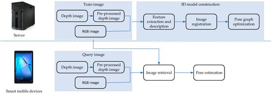
Figure 1.
Flow chart of the whole work.
In recent years, several scholars have published their own research in the field of visual positioning as well. Wan et al. [10] proposed an improved random sample consensus (RANSAC) method for indoor visual localization. They defined a function to measure the matching quality of matched image pairs. According to the matching quality, the four best matching pairs are selected to calculate the projection transformation matrix of the two images to eliminate false matching. Cheng et al. [11] proposed a location method based on the 3D structure and presented a two-stage outlier filtering framework using the visibility and geometric characteristics of a SfM point cloud for urban-scale location of tens of millions of points. Salarian et al. [12] used SfM to reconstruct the 3D camera position and improved the convergence speed of the SfM by using the criterion of the highest intra-class similarity between the images returned from the retrieval method. Then, the selected image and the query are used to reconstruct the 3D scene, and the relative camera position is determined by the SfM. In addition, an effective camera coordinate transformation algorithm was introduced to estimate the query geo-tag. Guan et al. [13] proposed an indoor positioning system that can be divided into two stages: offline and online. In the offline phase, feature points in speeded up robust features (SURF) format and line features are extracted to establish an image database, while in the online phase, the homography matrix and line features are used to estimate the position and direction. This method reduces the storage cost of the database and reduces the delay in practical applications. Kawamoto et al. [14] proposed a voting-based image similarity algorithm for image retrieval, which is robust to image geometric transformation and occlusion. To improve the performance of image retrieval, multiple voting, and ratio testing are introduced. Moreover, a particle filter is introduced to smoothly estimate the trajectory of the moving camera for the vision location. Feng et al. [15] established a visual map database that included visual features and corresponding location features. Subsequently, the query images of the two users were matched with the two database images, and the position and pose of the query camera were obtained using the inertial measurement unit (IMU) and electronic compass device on the smartphone.
Çinaroğlu et al. [16] obtained the semantic descriptor through semantic segmentation and subsequently used the approximate nearest neighbor search for localization. The success of this method is compared with the local descriptor-based method commonly used in the literature. On this basis, a hybrid method that combines the two methods was proposed.
Kim et al. [17] proposed a location method based on image and map data, which is suitable for various environments. To realize the localization process, they used an image-based localization method and Monte Carlo localization method with an a priori map database. The experimental results show that the open dataset has a satisfactory effect in various environments. To overcome the resource limitations of mobile devices, Tran et al. [18] designed a system that takes advantage of the scalability of image retrieval and positioning accuracy based on a 3D model. A novel cascading search algorithm based on a hash was proposed to rapidly calculate the corresponding relationship from 2D to 3D. Furthermore, a novel multiple RANSAC algorithm was proposed to achieve accurate angle estimation. This solves the challenge of repeated building structures in urban environment positioning.
Feng et al. [19] used an RGB-D sensor to build a visual map that contains the basic elements of image-based positioning, including camera posture, visual features, and 3D structure of buildings. Using the matched visual features and corresponding depth values, a novel local optimization algorithm is proposed to realize point cloud registration and pose estimation of the database camera. Then, the global consistency of the mapping was obtained by graph optimization. Based on a visual map, the image-based localization method is studied using the epipolar constraint. He et al. [20] proposed a six degree-of-freedom (6-DOF) pose estimation for a portable 3D vision sensor installed on mobile devices. A detailed 3D model of the indoor environment and a Wi-Fi received signal strength model are established in the offline training phase. In the online positioning process, the authors first use a Wi-Fi signal to locate the device in the 3D sub-model. Then, 6-DOF angle estimation is calculated by feature matching between the two-dimensional image collected online and the key frame image used to build the 3D model.
In addition, there is a great deal of work using deep learning methods to evaluate image similarity for the purpose of positioning. Xia et al. proposed a supervised hash code image retrieval method based on image expression learning [21]. This method does not need to use artificially defined visual features in feature extraction, and takes the lead in using deep neural network to extract image features. Lai et al. proposed a deep supervised hashing for fast image retrieval [22], which extracts image feature data and hash code by using image tag and other auxiliary information. In order to meet the performance requirements of large-scale image retrieval system, Liang et al. proposed a deep hashing for compact binary codes Learning [23], which extracts the nonlinear relationship between similar images through deep neural network. Liu et al. proposed a deep supervised hashing for fast image retrieval [24] to learn the similarity semantic relationship between image feature expression and hash code by using labeled image data as objects.
The organization of this paper is as follows. The methods of 3D model construction, image retrieval and pose estimation are presented in Section 2, Section 3 and Section 4. Section 5 describes the experimental environments and datasets and discusses the experimental results. The conclusion is offered in Section 6.
2. Construction of 3D Model
2.1. Feature Point Extraction and Description
In a real scene, color and depth images are captured together. To establish the association between different images, feature points must be extracted from the image and analyzed. Subsequently, image registration, and other operations can be performed to calculate the pose of each image, which can be used as the basis of visual positioning. There are numerous algorithms for feature point extraction and description. Here, we chose the ORB algorithm with both accuracy and efficiency. ORB, whose full name is oriented features from the accelerated segment test (FAST) and rotated binary robust independent elemental features (BRIEF), is a fast feature extraction and description algorithm proposed by Ethan Rublee et al. [25]. Feature extraction is developed from FAST algorithm [26], and feature description is improved based on the BRIEF algorithm [27]. This has been improved and optimized on its original basis. Compared with other feature extraction methods, such as scale-invariant feature transform (SIFT) [28] and speeded up robust features (SURF) [29], the speed of ORB is approximately 100 times that of SIFT and 10 times that of SURF.
2.2. Image Registration
Previously, we conducted the extraction and matching of feature points between images, after which we could register the images. Suppose we have two frames, and Moreover, we obtain two sets of one-to-one corresponding feature points:
where and are points in .
This problem aims to find a rotation matrix and displacement vector such that:
In fact, owing to the existence of errors, it is impossible for the left and right sides to be equal. The rotation and displacement vectors must be solved by minimizing the following errors:
This problem is solved using the perspective-n-point (PnP) method [30]. PnP is a method used for solving the motion from 3D to 2D point pairs. There are numerous methods for solving PnP problems, such as perspective-3-point (P3P) [31], efficient PnP (EPnP) [32], and universal PnP (UPnP) [33]. Here, we used the P3P method to calculate motion.
2.3. Pose Graph Optimization
The pose graph, as the name suggests, is a graph composed of a camera pose. The graph here is based on graph theory. It consists of nodes and edges:
In the simplest case, the node represents each pose (quaternion form) of the camera:
Edge refers to the transformation between two nodes:
The figure below shows a schematic diagram of the pose map in the process of the 3D model construction:

This is because there are errors in the edge , which makes the data given by all edges inconsistent. In the process of pose graph optimization, the inconsistency error must be optimized:
where is the estimate of . In the optimization process, they had an initial value. Then, according to the gradient of the objective function to :
The value of is adjusted to reduce . If this problem converges, the change in will be smaller, and will converge to a minimum. During this iteration, the change in the value of is .
Thus far, the problem can be abstracted as a nonlinear optimization problem. This problem is also called bundle adjustment (BA) [34], and the Levenberg Marquardt (LM) [35] method is usually used to optimize the nonlinear square error function.
3. Image Retrieval
3.1. Feature Clustering
In the process of building the 3D model, feature points are extracted from all sample images. In the image retrieval stage, based on these extracted feature points, we must cluster the feature points to obtain a codebook. Then, the codebook is used to map the original n-dimensional feature vector to the k-dimensional space. The results of the clustering algorithm affect the quality of the codebook, which is crucial for the subsequent retrieval process. Clustering is an unsupervised learning algorithm. Its essence is to automatically classify similar objects into the same cluster without any additional training. Here we use the K-means algorithm to cluster the features. The most significant feature of this algorithm is that it is easy to understand and runs fast.
The process of feature clustering algorithm is as follows:
Step 1: Randomly select sample points as the center of each cluster. . The distance between the center points is set as far as possible.
Step 2: Calculate the distance between all sample points and the center of the clusters. Then, all points are divided into the nearest cluster center according to the nearest-neighbor principle. The formula below represents the process of dividing the sample points into cluster centers:
where is the th sample point, is the th cluster center, and is the cluster center assigned to the th sample point.
Step 3: Recalculate the cluster center of each class according to their existing objects. The calculation formula is given below:
Step 4: Repeat steps 2–3 until the position of the cluster center is almost unchanged, and the cluster center is the center of the feature point.
To ensure the convergence of the feature clustering algorithm, a loss function must be defined:
It represents the square sum of the distances from each sample point to the cluster center. The ideal result of the feature clustering algorithm is to minimize the loss function. If the current loss function does not reach the minimum value, we can first maintain the cluster center of each cluster. The cluster center point of each sample point was adjusted to reduce the objective function. In contrast, remains unchanged, while a change in can likewise reduce the loss function. As the formula above is a nonconvex function, the clustering algorithm may not reach the global minimum, but converge to the local minimum instead. In this case, we must run the feature clustering algorithm numerous times, randomly select the cluster center point each time, and subsequently select the smallest center point in the final result.
3.2. Feature Coding
After obtaining the codebook, we can start to encode the features, which aims to reduce the large amount of noise generated during feature extraction. This process removes redundant information and simplifies the feature representation vector. Feature coding not only improves the expressiveness of the vector, better expresses an image but also generates a unified and standardized contrast template, which is conducive to the establishment of an index in the subsequent image retrieval.
It is a prerequisite for the image retrieval process to represent an image as a vector. An image vector representation method based on local visual features was employed. The specific steps are as follows:
Step 1: Read the image file. The local feature descriptor of the image was extracted and recorded as . For an image database with n sample size, we first extract local feature descriptors from all images, assuming that the number of local features extracted is n, and each local feature descriptor is 128 dimensions; then, all the descriptors are extracted from a dimensional matrix.
Step 2: Use the feature clustering algorithm to cluster the extracted descriptors to generate a visual dictionary. Set the number of cluster centers as and the visual words as .
Step 3: Quantize each local feature and divide it to the nearest cluster center using the K-D tree [36] data structure:
where is the cluster center assigned to .
Step 4: Calculate the residual of the cluster center and local features, sum all the residuals of each image on the same cluster center, and then normalize them. Finally, each cluster center obtains a residual sum. If every local feature descriptor is 128 dimensional, then the sum of residuals is also a 128-dimensional vector. We define the vector as S. Different features may exhibit different signs.
Step 5: Sum the residuals. The formula of residual sum is expressed as follows:
where is the residual sum of the th cluster center.
Step 6: Splice the sum of residuals to generate a long vector with a length of . After normalization, the vector of the local aggregated descriptors (VLAD) [37] is obtained.
3.3. Combining Color and Depth Information in the Vector of the Locally-Aggregated Descriptor (VLAD)
Our feature coding method is the algorithm of the feature coding stage of image retrieval in this study; it is both fast and efficient. However, some useful information is lost in the process of feature description, which weakens the ability to distinguish feature points. This leads to incorrect matching in the process of image matching and affects the final retrieval effect.
To solve the above problem, we added the color information of the picture in the feature coding stage, such that the coding vector contains the color information. In contrast, our visual positioning image acquisition equipment not only has an RGB camera but also a depth camera such that the depth information is likewise a very important tool for improving the positioning accuracy. We further added depth information in the feature coding stage such that the coding vector includes depth information. In the feature coding stage, we aggregated the features that we extracted previously, and the significance of aggregation is to simplify the number of features. In the image, the dimension of the binary descriptor extracted by the ORB operator is 128, so a dimension vector of locally aggregated descriptor (VLAD) of the image can be obtained after feature coding, which significantly reduces the computational complexity compared with the large ORB feature descriptor. In this scenario, the combination of the VLAD vector with the color information extracted from the image, and the depth information extracted from the depth image will not significantly increase the time cost and will not occupy a substantial amount of memory. While ensuring the matching speed, this increases the utilization of valuable information of the image, improves the robustness of color and depth, and strengthens the discrimination of each image feature vector. It can also achieve a better image retrieval effect in an environment of illumination and scale changes.
In the process of improving the VLAD feature coding algorithm for image retrieval, the input RGB image is first converted into a gray image, and then the values of the three channels in the RGB image are transformed into the opponent color space to obtain , , , and the image matrix corresponding to the three color channels. The opponent color space is one of the most outstanding mainstream color descriptors [38]. The opponent decomposes the color space into three channels, namely, , and . Each channel is described by a descriptor. The conversion method from RGB space to opponent space is expressed in the following formulae:
Here, and channels contain red-green and blue-yellow opponent colors, respectively, which have good invariance to the brightness of the image. The channel contains the intensity information of the color space, which is affected by the scale factor. The above three-color channels constitute the opponent color space. In real scenes of daily life, the changes of lighting conditions include the changes of brightness conditions and color conditions. The opponent color space contains three channels. O1 and O2 channels contain red-green and yellow-blue component colors respectively, which have good invariance to the brightness of the image. They are robust when the brightness condition changes. The O3 channel is the intensity information, and the value of the O3 channel will not change when the color condition changes. In short, the opponent color space can enhance the robustness of image retrieval under different lighting conditions.
Adding three channels of color information in the feature coding stage of image retrieval not only maintains the efficiency of the ORB binary descriptor but also improves the robustness of the image retrieval structure to color.
In the process of VLAD coding, the ORB descriptors of each image are assigned to all cluster centers according to the nearest neighbor principle, and there are several ORB descriptors in each cluster center. We take the nearest feature descriptor from each cluster center as the color and depth key point of the image and extract the color information and depth information using binary coding. For each key point , the 3 × 3 region R with the key feature point as the center is selected from the corresponding image matrix of , , and color channels, respectively, and the mean value of the corresponding color channel of each region is calculated. Similarly, another 3 × 3 region R with the key feature point as the center is selected on the depth image, and the mean of the depth value of each region is obtained. The calculation is carried out according to the following formulae:
where represents the three color channels of the image, with 1, 2, and 3; is the number of points in region R, with a total of nine feature points; represents the mean value of region R on the th color channel of the image; represents the value of the th color channel of the th feature point on the image; represents the mean value of region R of the depth image; and represents the value of the th feature point on the depth image.
After obtaining the mean value of each color channel of region R around the color key point of the image, the color and depth binary coding corresponding to the key point is generated:
where represents the binary color coding of the th feature point on the th color channel of the image. The value of each color channel of each feature point in the neighborhood R centered on the key point is compared with the channel mean value of region R. If the value of the point is less than the channel mean value of the region, the binary code of the point is 0. If the value of the point is larger than the channel mean value of the region, the binary code of the point is 1. represents the binary encoding of the th feature point in the corresponding depth image. The depth value of each feature point in the neighborhood R centered on the key point is compared with the mean depth value of the region R. If the value of the point is less than the mean depth of the region, the binary code is 0; if it is greater than the mean, the binary code is 1. Each color channel has nine binary codes, a total of three color channels, and a depth channel. In particular, a picture has 36 codes.
After the above operations on a picture, the binary coding of the picture in three opponent color channels and depth channels is obtained. After obtaining the color binary coding of all the regions around the color key points, it is added to the original VLAD representation vector such that a new vector with a length of is obtained, which is the improved VLAD feature coding vector. The process of obtaining the improved VLAD feature code is shown in Figure 2.
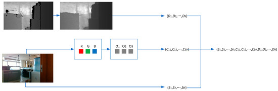
Figure 2.
Improved VLAD coding framework.
3.4. Similarity Measurement
The results of image retrieval were sorted according to the rules used to measure the similarity between images. To evaluate whether two images match, we must use a similarity measure to calculate the similarity between images. The similarity measure calculates the distance between the sample descriptor vectors and sorts them after obtaining the image feature coding descriptor.
As the descriptor vector in this study is binary, to evaluate the similarity more efficiently, the Hamming distance [39] of the distance between the measurement vectors is employed. The Hamming distance is used to calculate the similarity of two vectors; that is, by comparing whether each bit of the vector is the same, if it is different, Hamming distance is added by one to obtain the Hamming distance. The higher the vector similarity, the smaller the corresponding Hamming distance:
where denotes the Hamming distance of the two descriptor vectors , which are bit codes. Further, denotes the XOR operation.
4. Pose Estimation
After retrieving the most similar image, there is a certain difference between it and the pose of the handheld device, explained in a conversion relationship between the poses of the two images. Therefore, in this process, a rotation matrix and translation matrix are required. As the 3D model of the scene has been generated by the scene image library, the most similar image has its corresponding 3D point cloud. The pose solving problem here aims to solve the rotation and translation matrix between a given 3D point cloud and an image. This case is a 2D–3D problem that can be solved by PnP.
The homogeneous equation of the high-space point is . Let it project to feature point . To solve and , the augmented matrix is defined; after expanding the equation, we obtain the following results:
After eliminating , the constraint is obtained:
Assume that:
so:
.
Here, is a variable. A feature point can provide two constraints on if there are feature points; the following equation holds:
where has 12 variables and the solution of T can be obtained by at least six pairs of matching points. Hence, this method is referred to as the direct linear transformation method; when the matching points are more than six pairs, singular value decomposition (SVD) [40] methods can be used to solve the overdetermined equation.
The solution T is composed of R and t, so R satisfies R = SO(3). Hence, we must find the best rotation matrix for the T matrix, which can be completed by QR decomposition [41], which is equivalent to ghost the result from the matrix space to the SE(3) manifold, and transform it into rotation and translation.
5. Experiment
In this section, we introduce the experimental environments and datasets we used, present the visual positioning results of the proposed method as well as the original VLAD method, and then compare them.
5.1. Experimental Environments and Datasets
The algorithms were launched on a computer with an Intel i5 2.50 GHz CPU, 8 GB RAM. The computer has installed the Ubuntu 16.04 LTS operating system, which is a widely used open-source operating system. The code was written in the C++ language.
To verify the effectiveness of the proposed algorithm, the experiments were performed on the Intel RealSense D435i (manufacturer: Intel Co., Ltd., Santa Clara, CA, USA) depth images of several public datasets and compared with the algorithms of VLAD [37]. OpenLORIS-Scene datasets [42], created by researchers at the Inter Research Center and Tsinghua University, have RGB and depth images collected by RealSense D435i with a resolution of 848 × 480 and data from an inertial measurement unit, a fish-eye camera, and a wheel odometer. The data of each sensor were collected at the same time. This study used the RGB and depth image data. The depth image was processed and aligned with the RGB image. We synthesized the ground truths through artificial restoration, referencing information from RGB images. Datasets of five scenes were used: home, cafe, office, and corridor environments.
5.2. Experimental Results and Comparison
In the four scenes of home, cafe, office and corridor of LORIS data set, the RGB-D images data with moderate daylight intensity is selected to construct the 3D model. The data set with moderate illumination can reduce the difficulty of model construction and pose estimation, and has better effect and higher accuracy. This is beneficial to the subsequent use of these postures as the basis for visual positioning. The three-dimensional model of the four scenes is shown in Figure 3.
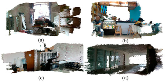
Figure 3.
Three-dimensional model constructed from RGB-D image: (a) Home scene; (b) cafe scene; (c) office scene; (d) corridor scene.
In the image retrieval stage, this experiment selects two images as the images to be retrieved in each of the four scenes mentioned above. Each image was retrieved by VLAD and our proposed method, a total of eight times. The first similarity image is displayed as the result. The images to be retrieved and the images previously constructed in the image retrieval training set are taken under different lighting conditions. In this way, we can effectively compare the image retrieval effect under the condition of light change, and the difference between the two methods.
In the home scene, we selected two photos taken when the lights were on at night as the query set images. The images in the training set are taken when the light is not on in the daytime. The lighting conditions of the query set and the training set are different. Figure 4 shows the most similar image (that is, the image with the smallest Hamming distance) retrieved each time after the two images are retrieved by VLAD method and our proposed method. For the first image of the query set, VLAD method searches out the wardrobe. There is still a distance between the inquired pictures and the wardrobe, which only accounts for a small part. The result of our proposed method is very close to the query image. The second image of the query set is taken in front of the wardrobe. The retrieval results of the two methods are mainly pictures of the wardrobe. The images retrieved by our proposed method are closer to those retrieved.
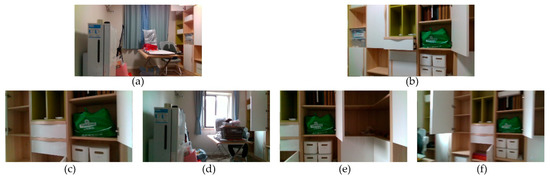
Figure 4.
Query images in home scene and query results; (a) Query image no. 1; (b) query image no. 2; (c) query result of image 1 with the VLAD method; (d) query result of image 1 with our proposed method; (e) query result of image 2 with the VLAD method; (f) query result of image 2 with our proposed method.
Since the lighting conditions of each dataset of the cafe scene are almost the same, the lighting conditions of the query set and the training set are similar. Figure 5 shows the most similar images retrieved each time after the two images are retrieved by VLAD method and our proposed method. The first image of the query set is taken in front of the bar near the seat. The image retrieved by VLAD method is taken behind the bar, which is a little different from the image being queried. The image retrieved by our proposed method is in front of the bar, which is similar to the image being retrieved. For the second image, the retrieval results of the two methods are similar to the retrieved image, and the results of this method are similar.
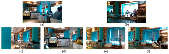
Figure 5.
Query images in cafe scene and query results: (a) Query image no. 1; (b) query image no. 2; (c) query result of image 1 with the VLAD method; (d) query result of image 1 with our proposed method; (e) query result of image 2 with the VLAD method; (f) query result of image 2 with our proposed method.
In the office scene, two photos taken in a narrow space with weak light are selected as the query set images. The illumination condition of training set image is moderate. Figure 6 shows the retrieval results of the two methods. For the first image in the query set, the distance between the retrieve result by VLAD and the query image is far, and the two images have no common feature points, so it is impossible to use PnP to solve the pose. The retrieve results by our proposed method are very close to retrieved images. For the second image of the query set, the images retrieved by the two methods are similar to the query image.
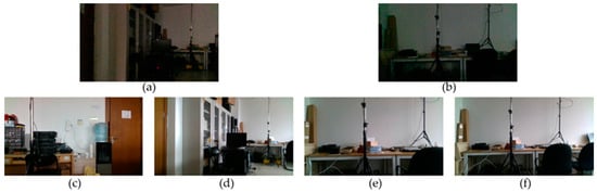
Figure 6.
Query images in office scene and query results: (a) Query image no. 1; (b) query image no. 2; (c) query result of image 1 with the VLAD method; (d) query result of image 1 with our proposed method; (e) query result of image 2 with the VLAD method; (f) query result of image 2 with our proposed method.
In the corridor scene, two photos taken under strong sunlight conditions are selected as query set images. The illumination condition of training set image is moderate. Figure 7 shows the retrieval results of the two methods. Generally speaking, the retrieved images are similar to the retrieved images. However, the retrieval result of the second image in the query set is quite different from it.
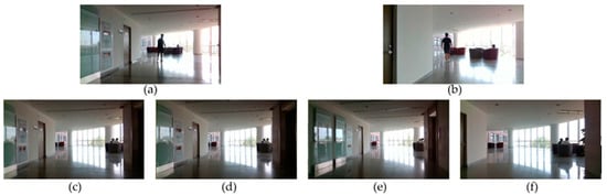
Figure 7.
Query images in corridor scene and query results: (a) Query image no. 1; (b) query image no. 2; (c) query result of image 1 with the VLAD method; (d) query result of image 1 with our proposed method; (e) query result of image 2 with the VLAD method; (f) query result of image 2 with our proposed method.
After the completion of image retrieval, we choose images ranked first in each scene query result to estimate the pose. In the early stage, we have generated the 3D model of the scenes. We extract the corresponding 3D point cloud of the query result. The point cloud and the retrieve result image are used for 3D-2D pose calculation, using PnP method. Since the images in the train sets have known 6-DOF pose, the 6-DOF pose of the query image can be known by calculating the displacement matrix and rotation matrix between the query image and the query result. Table 1 shows the three-dimensional coordinates of each query image in the four scenes of home, cafe, office and corridor by VLAD and our proposed method, as well as the error compared with the ground true value. It can be seen that the coordinate errors of VLAD method are relatively large. Some of them have errors of 5–6 m. In addition, because the query result of the fifth image does not have the same feature points with the queried image, its pose cannot be calculated. The errors of our proposed method are relatively small, and the maximum error is about two meters. Compared with the original VLAD method, it has been greatly improved.

Table 1.
Pose estimation result of VLAD and our proposed method (position, unit: m).
Table 2 shows the angle of each query image in the four scenes calculated by VLAD and proposed method (expressed by quaternion for convenience of calculation), together with the errors compared with ground true value. Although the errors of the two methods are small, the results of VLAD method are relatively large. Compared with the original VLAD method, the error of the proposed method is relatively small.
Table 2.
Pose estimation result of VLAD and our proposed method (angle, quaternion form).
ORB-SLAM2 is another state-of-the-art positioning method proposed by Mur-Artal and Tardós [43]. It uses feature descriptor and extractor to tracking for real-time localization and mapping. It supports monocular, stereo and RGB-D camera data. Table 3 and Table 4 shows the position and angle estimation result of ORB-SLAM2 method. Most of the errors are larger than those of our proposed method. It shows that the positioning effect of our proposed method is better.
Table 3.
Pose estimation result of ORB-SLAM2 method and our proposed method (position, unit: m).
Table 4.
Pose estimation result of ORB-SLAM2 method and our proposed method (angle, quaternion form).
Table 5 shows the average error and average positioning time of the three methods. Because the proposed method expands the capacity of VLAD descriptor, it takes a little more time than the original VLAD, but it is still at a very efficient level. ORB-SLAM2 is faster than VLAD. Compared with the original VLAD method and ORB-SLAM2, the proposed method improves the positioning accuracy greatly when the illumination conditions of the query set and the training set are different.
Table 5.
Mean error and retrieval time of VLAD and the proposed method.
6. Conclusions and Discussion
In this paper, we proposed a visual positioning method using RGB-D image on smart mobile devices. In this paper, we improve the VLAD image retrieval method, which is applied to mobile vision positioning. This method has the advantages of small memory consumption, fast calculation speed and high accuracy. Firstly, the pose of each image in the training set is calculated through ORB feature extraction and description, image registration, and pose map optimization. Then, in the image retrieval stage, the training set and the query set are clustered to generate the VLAD description vector. In order to overcome the problem that the description vector loses the image color information and improve the retrieval accuracy under different lighting conditions, we combined the color information and depth information with VLAD descriptors for image retrieval. It is robust when the brightness condition and color condition changes. Opponent color space, together with depth information, can enhance the robustness of image retrieval under different lighting conditions. Finally, the 6-DOF pose of the query images are calculated by PnP method with query image and retrieve result image. Experiments are carried out on RGB-D data of four scenes (cafe, corridor, home and office) in LORIS dataset. The results under different illumination conditions in indoor scenes show that the proposed method improves the positioning accuracy compared with the original VLAD and ORB-SLAM2, which has good computational efficiency. On the other hand, another experiment by us shows that when using only depth information without color component, the position estimation errors of 8 query images are 0.300, 0.552, 2.457, 0.417, 3.076, 0.497, 0.928, and 3.764. The errors are larger than those with color component.
Due to the limited time and energy of the author, it is impossible to propose a perfect technology in indoor positioning. Therefore, there are still some research contents in this field that need to be improved and supplemented. At present, the efficiency of the proposed method needs to be improved. In the later research, we will try to use hierarchical clustering instead of the existing k-means clustering to improve the efficiency. In order to improve the accuracy, we may do some research using deep learning method. On the other hand, we also need to study a positioning method which is less dependent on the server to avoid wasting time in the process of network transmission.
There may be some occlusion in the query image taken by the mobile device users. They will increase the difficulty of image retrieval to a certain extent, and also affect the accuracy of position estimation algorithm. Therefore, in future work, we will study the visual feature filtering algorithm in the case of occlusion, and attempt to improve the positioning accuracy through the visual feature filtering algorithm.
Author Contributions
Longyu Zhang and Hao Xia designed the visual positioning method. Longyu Zhang, Hao Xia, and Qingjun Liu developed the software. Longyu Zhang and Dong Fu performed the experi-ments. Longyu Zhang and Chunyang Wei summarized the development of visual positioning an-alyzed the data. Longyu Zhang, Chunyang Wei, and Yanyou Qiao wrote the paper. All authors have read and agreed to the published version of the manuscript.
Funding
This work was supported by the National Key Research and Development Plan (no. 2017YFC0821900).
Institutional Review Board Statement
Not applicable.
Informed Consent Statement
Not applicable.
Data Availability Statement
The data presented in this study are available from the author upon reasonable request.
Acknowledgments
Special thanks are given to the anonymous reviewers and editors for their constructive comments.
Conflicts of Interest
The authors declare no conflict of interest.
References
- Franz, M.O.; Mallot, H.A. Biomimetic robot navigation. Robot. Auton. Syst. 2000, 30, 133–153. [Google Scholar] [CrossRef]
- Seo, P.H.; Weyand, T.; Sim, J.; Han, B. CPlaNet: Enhancing image geolocalization by combinatorial partitioning of maps. In Lecture Notes in Computer Science; Springer: Berlin, Germany, 2018; pp. 544–560. [Google Scholar]
- Microsoft. Kinect. Available online: http://www.xbox.com/en-us/kinect/ (accessed on 28 September 2020).
- Qin, X.; Ge, Y.; Feng, J.; Yang, D.; Chen, F.; Huang, S.; Xu, L. DTMMN: Deep transfer multi -metric network for RGB-D action recognition. Neurocomputing 2020, 406, 127–134. [Google Scholar] [CrossRef]
- Shamwell, E.J.; Lindgren, K.; Leung, S.; Nothwang, W.D. Unsupervised deep visual-inertial odometry with online error correction for RGB-D imagery. IEEE Trans. Pattern Anal. Mach. Intell. 2020, 42, 2478–2493. [Google Scholar] [CrossRef] [PubMed]
- Ingman, M.; Virtanen, J.-P.; Vaaja, M.T.; Hyyppä, H. A comparison of low-cost sensor systems in automatic cloud-based indoor 3D modeling. Remote Sens. 2020, 12, 2624. [Google Scholar] [CrossRef]
- Park, K.B.; Choi, S.H.; Kim, M.; Lee, J.Y. Deep learning-based mobile augmented reality for task assistance using 3D spatial mapping and snapshot-based RGB-D data. Comput. Ind. Eng. 2020, 146, 106585. [Google Scholar] [CrossRef]
- Ahn, M.S.; Chae, H.; Noh, D.; Nam, H.; Hong, D. Analysis and Noise Modeling of the Intel RealSense D435 for Mobile Robots. In Proceedings of the 16th International Conference on Ubiquitous Robots (UR), Jeju, Korea, 24–27 June 2019. [Google Scholar]
- Soille, P. Morphological Image Analysis: Principles and Applications. Sens. Rev. 1999, 28, 800–801. [Google Scholar]
- Wan, K.; Ma, L.; Tan, X. An Improvement Algorithm on RANSAC for Image-Based Indoor Localization. In Proceedings of the 2016 International Wireless Communications and Mobile Computing Conference (IWCMC), Paphos, Cyprus, 5–9 September 2016; pp. 842–845. [Google Scholar]
- Cheng, W.; Lin, W.; Sun, M.T. 3D Point Cloud Simplification for Image-Based Localization. In Proceedings of the 2015 IEEE International Conference on Multimedia & Expo Workshops (ICMEW), Turin, Italy, 29 June 2015; pp. 1–6. [Google Scholar]
- Salarian, M.; Iliev, N.; Cetin, A.E.; Ansari, R. Improved image-based localization using SfM and modified coordinate system transfer. IEEE Trans. Multimed. 2018, 20, 3298–3310. [Google Scholar] [CrossRef]
- Guan, K.; Ma, L.; Tan, X.; Guo, S. Vision-Based Indoor Localization Approach Based on SURF and Landmark. In Proceedings of the 2016 International Wireless Communications and Mobile Computing Conference (IWCMC), Paphos, Cyprus, 5–9 September 2016; pp. 655–659. [Google Scholar]
- Kawamoto, K.; Kazama, H.; Okamoto, K. Visual Localization Using Voting Based Image Retrieval and Particle Filtering in Indoor Scenes. In Proceedings of the 2013 Second International Conference on Robot, Vision and Signal Processing, Kitakyushu, Japan, 10–12 December 2013; pp. 160–163. [Google Scholar]
- Feng, G.; Tan, X.; Ma, L. Visual Location Recognition Using Smartphone Sensors for Indoor Environment. In Proceedings of the 2015 10th International Conference for Internet Technology and Secured Transactions (ICITST), London, UK, 14–16 December 2015; pp. 426–430. [Google Scholar]
- Çinaroğlu, İ.; Baştanlar, Y. Image Based Localization Using Semantic Segmentation for Autonomous Driving. In Proceedings of the 2019 27th Signal Processing and Communications Applications Conference (SIU), Sivas, Turkey, 24–26 April 2019; pp. 1–4. [Google Scholar]
- Kim, H.; Oh, T.; Lee, D.; Myung, H. Image-Based Localization Using Prior Map Database and Monte Carlo Localization. In Proceedings of the 2014 11th International Conference on Ubiquitous Robots and Ambient Intelligence (URAI), Kuala Lumpur, Malaysia, 12–15 November 2014; pp. 308–310. [Google Scholar]
- Tran, N.T.; Le Tan, D.K.; Doan, A.D.; Do, T.T.; Bui, T.A.; Tan, M.; Cheung, N.M. On-Device Scalable Image-Based Localization Via Prioritized Cascade Search and Fast One-Many RANSAC. IEEE Trans. Image Process. 2018, 28, 1675–1690. [Google Scholar] [CrossRef] [PubMed]
- Feng, G.; Ma, L.; Tan, X. Visual map construction using RGB-D sensors for image-based localization in indoor environments. J. Sens. 2017, 2017, 1–18. [Google Scholar] [CrossRef]
- He, X.; Aloi, D.; Portable, L.J. 3D Visual Sensor Based Indoor Localization on Mobile Device. In Proceedings of the 2016 13th IEEE Annual Consumer Communications & Networking Conference (CCNC), Las Vegas, NV, USA, 9–12 January 2016; pp. 1125–1128. [Google Scholar]
- Xia, R.; Pan, Y.; Lai, H.; Liu, C.; Yan, S. Supervised hashing for image retrieval via image representation learning. Proc. AAAI Conf. Artif. Intell. 2014, 28, 2156–2162. [Google Scholar]
- Lai, H.; Pan, Y.; Liu, Y.; Yan, S. Simultaneous feature learning and hash coding with deep neural networks. In Proceedings of the 2015 IEEE Conference on Computer Vision and Pattern Recognition, Boston, MA, USA, 7–12 June 2015; pp. 3270–3278. [Google Scholar]
- Erin, L.V.; Lu, J.; Wang, G.; Moulin, P.; Zhou, J. Deep hashing for compact binary codes learning. In Proceedings of the IEEE conference on Computer Vision and Pattern Recognition, Boston, MA, USA, 7–12 June 2015; pp. 2475–2483. [Google Scholar]
- Liu, H.; Wang, R.; Shan, S.; Chen, X. Deep supervised hashing for fast image retrieval. In Proceedings of the IEEE Conference on Computer Vision and Pattern Recognition, Las Vegas, NV, USA, 27–30 June 2016; pp. 2064–2072. [Google Scholar]
- Rublee, E.; Rabaud, V.; Konolige, K.; Bradski, G. ORB: An Efficient alternative to SIFT or SURF. In Proceedings of the 2011 International Conference on Computer Vision, Barcelona, Spain, 6–13 November 2011; pp. 2564–2571. [Google Scholar]
- Viswanathan, D.G. Features from Accelerated Segment Test (Fast). In Proceedings of the 10th Workshop on Image Analysis for Multimedia Interactive Services, London, UK, 6–8 May 2009; pp. 6–8. [Google Scholar]
- Calonder, M.; Lepetit, V.; Strecha, C.; Fua, P.V. BRIEF: Binary Robust Independent Elementary Features. In European Conference on Computer Vision; Springer: Berlin/Heidelberg, Germany, 2010; pp. 778–792. [Google Scholar]
- Lowe, G. SIFT-the scale invariant feature transform. Int. J. 2004, 2, 91–110. [Google Scholar]
- Bay, H.; Ess, A.; Tuytelaars, T.; Van Gool, L. Speeded-up robust features (SURF). Comput. Vis. Image Underst. 2008, 110, 346–359. [Google Scholar] [CrossRef]
- Wu, Y.; Hu, Z. PnP Problem Revisited. J. Math. Imaging Vis. 2006, 24, 131–141. [Google Scholar] [CrossRef]
- Gao, X.; Hou, X.; Tang, J.; Cheng, H. Complete Solution Classification for the Perspective-Three-Point Problem. IEEE Trans. Pattern Anal. Mach. Intell. 2003, 25, 930–943. [Google Scholar]
- Lepetit, V.; Moreno-Noguer, F.; Fua, P. EPnP: An Accurate O(n) Solution to the PnP Problem. Int. J. Comput. Vis. 2009, 81, 155–166. [Google Scholar] [CrossRef]
- Kneip, L.; Li, H.; Upnp, S.Y. An Optimal o (n) Solution to the Absolute Pose Problem with Universal Applicability. In European Conference on Computer Vision; Springer: Cham, Switzerland, 2014; pp. 127–142. [Google Scholar]
- Triggs, B.; McLauchlan, P.F.; Hartley, R.I.; Fitzgibbon, A.W. Bundle Adjustment—A Modern Synthesis. In Lecture Notes in Computer Science International Workshop on Vision Algorithms; Springer: Berlin/Heidelberg, Germany, 2000; pp. 298–372. [Google Scholar]
- Moré, J.J. The Levenberg-Marquardt algorithm: Implementation and theory. In Lecture Notes in Mathematics; Springer: Berlin/Heidelberg, Germany, 1978; pp. 105–116. [Google Scholar]
- Moore, A.W. An Introductory Tutorial on K-D Trees. 1991. Available online: http://www.autonlab.org/autonweb/14665 (accessed on 23 March 2021).
- Jégou, H.; Douze, M.; Schmid, C.; Pérez, P. Aggregating Local Descriptors into a Compact Image Representation. In Proceedings of the 2010 IEEE Computer Society Conference on Computer Vision and Pattern Recognition, San Francisco, CA, USA, 13–18 June 2010; pp. 3304–3311. [Google Scholar]
- Van de Sande, K.E.A.; Gevers, T.; Snoek, C.G.M. Evaluating color descriptors for object and scene recognition. IEEE Trans. Pattern Anal. Mach. Intell. 2010, 32, 1582–1596. [Google Scholar] [CrossRef] [PubMed]
- Norouzi, M.; Fleet, D.J.; Salakhutdinov, R.R. Hamming distance metric learning. Adv. Neural Inf. Process. Syst. 2012, 25, 1061–1069. [Google Scholar]
- Paige, C.C.; Saunders, M.A. Towards a generalized singular value decomposition. SIAM J. Numer. Anal. 1981, 18, 398–405. [Google Scholar] [CrossRef]
- Gander, W. Algorithms for the QR Decomposition. Res. Reprod. 1980, 80, 1251–1268. [Google Scholar]
- Shi, X.; Li, D.; Zhao, P.; Tian, Q.; She, Q. Are We Ready for Service Robots? The OpenLORIS-Scene Datasets for Lifelong SLAM. In Proceedings of the International Conference on Robotics and Automation (ICRA), Montreal, QC, Canada, 20–24 May 2019; pp. 3139–3145. [Google Scholar]
- Mur-Artal, R.; Tardós, J.D. ORB-slam2: An open-source slam system for monocular, stereo, and RGB-D cameras. IEEE Trans. Robot. 2017, 33, 1255–1262. [Google Scholar] [CrossRef]


Publisher’s Note: MDPI stays neutral with regard to jurisdictional claims in published maps and institutional affiliations. |
© 2021 by the authors. Licensee MDPI, Basel, Switzerland. This article is an open access article distributed under the terms and conditions of the Creative Commons Attribution (CC BY) license (http://creativecommons.org/licenses/by/4.0/).