Article

Three-Dimensional Inundation Mapping Using UAV Image Segmentation and Digital Surface Model

by
Asmamaw A Gebrehiwot
1 and
Leila Hashemi-Beni
2,*
1
Applied Science & Technology PhD Program, North Carolina A&T State University, Greensboro, NC 27411, USA
2
Geomatics Program, North Carolina A&T State University, Greensboro, NC 27411, USA
*
Author to whom correspondence should be addressed.
ISPRS Int. J. Geo-Inf. 2021, 10(3), 144; https://doi.org/10.3390/ijgi10030144
Submission received: 27 December 2020 / Revised: 21 February 2021 / Accepted: 1 March 2021 / Published: 6 March 2021

Abstract

:
Flood occurrence is increasing due to the expansion of urbanization and extreme weather like hurricanes; hence, research on methods of inundation monitoring and mapping has increased to reduce the severe impacts of flood disasters. This research studies and compares two methods for inundation depth estimation using UAV images and topographic data. The methods consist of three main stages: (1) extracting flooded areas and create 2D inundation polygons using deep learning; (2) reconstructing 3D water surface using the polygons and topographic data; and (3) deriving a water depth map using the 3D reconstructed water surface and a pre-flood DEM. The two methods are different at reconstructing the 3D water surface (stage 2). The first method uses structure from motion (SfM) for creating a point cloud of the area from overlapping UAV images, and the water polygons resulted from stage 1 is applied for water point cloud classification. While the second method reconstructs the water surface by intersecting the water polygons and a pre-flood DEM created using the pre-flood LiDAR data. We evaluate the proposed methods for inundation depth mapping over the Town of Princeville during a flooding event during Hurricane Matthew. The methods are compared and validated using the USGS gauge water level data acquired during the flood event. The RMSEs for water depth using the SfM method and integrated method based on deep learning and DEM were 0.34m and 0.26m, respectively.

1. Introduction

Flooding is one of the most destructive natural disasters, the severity and frequency of which have increased in recent years due to the expansion of urbanization and extreme weather such as hurricanes [1]. For example, Hurricane Harvey in 2017 caused about $125 billion in damage in the U.S. and ranked as the second-most costly hurricane to affect the U.S. mainland since 1900 [2]. Hurricanes Irma and Maria followed within a month of Hurricane Harvey and brought widespread death and destruction to Florida, Puerto Rico, and the U.S. Virgin Islands, causing $50 billion and $90 billion in damages, respectively [3]. According to the National Hurricane Center report, 2017’s hurricanes caused more than a quarter-trillion dollars in insured and uninsured losses [4]. Thus, studying efficient methods to quickly estimate the magnitude of floods in terms of coverage area and inundation depth is compelling for effective emergency response and damage assessment activities [5,6].
A variety of remote sensing systems are capable of providing spatial data that are needed to create an inundation map [7,8]. However, critical factors such as spatial coverage, data acquisition timing, and image quality impact the operational suitability of these systems for flood mapping. Satellite remote sensing has been used as one of the powerful tools for inundation mapping. The increasing availability of satellite imagery allows the production of flood maps at a large scale [9,10]. However, the spatial resolution of freely available data such as Landsat and Sentinel is not good enough to create precise and detailed inundation maps, and very high-resolution satellite imagery such as QuickBird and Ikonos is relatively costly to acquire [11]. In addition, the acquisition of suitable optical imagery constrained by clouds, and the satellite’s regular trajectory, view angle, and their predefined schedule may fail to collect data at critical times, such as peak flood. With recent technological advances, unmanned aerial vehicles (UAV) have been considered as effective platforms for flood management applications. UAVs can acquire very high-resolution imagery with flexibility in the frequency and time of data acquisition [12]. In contrast, their short flight endurance and small-scale coverage remain areas of weakness for their wide-scale implementation in remote sensing.
The extraction of 2D flood extent has been extensively studied, and several methods have been developed to efficiently map inundation areas from remote sensing imagery [13,14,15,16]. Among these, convolutional neural networks (CNN) have shown promising results for 2D inundation mapping. CNNs are becoming popular techniques for remote sensing tasks due to their ability to automatically extract and learn directly from input data/images and successfully handle large datasets. Recent studies used CNNs for automatically extracting 2D inundation extent using remote sensing optical or Synthetic Aperture Radar (SAR) imagery [17,18,19,20,21]. For optical imagery, Gebrehiwot et al. [18] fine-tuned and trained Fully Convolutional Neural Networks (FCNs) to create a flood extent using UAV optical images and achieved more than 95% accuracy segmenting the flood in non-vegetated areas. Peng et al. [19] used a residual patch similarity convolutional neural network (ResPSNet) to map urban flood hazard zones using pre- and post-Hurricane Harvey flood imagery in Houston, Texas. They achieved a precision of 0.9002 and a recall of 0.9302. Sarker et al. [20] applied an FCN model to detect the inundation area using Landsat satellite images in Australia and achieved (76.7%) compared to SVM (45.27%) for the flood classification task. Wu et al. [21] proposed a multi-depth flood detection CNN (MDFD-CNN) to classify and extract the water region from SAR imagery. Kang et al. [22] fine-tuned an FCN to generate flood extent maps from Gaofen-3 SAR images and achieved more than 90% accuracy with a few training samples. Although the results demonstrate the highly promising potential of deep learning methods for inundation mapping, CNN methods, like other image classification approaches, are limited to extract only 2D flood extent, and water depth cannot be measured from 2D imagery. The water depth information is critical for flood management practices such as quantifying impacts and damages, better-characterizing flood risk, implementing disaster risk reduction measures, assessing accessibility and designing suitable intervention plans, calculating water volumes, and allocating resources for water pumping.
Satellite altimetry data are one of the data sources for estimating floodwater depth. Satellite altimetry measures the water’s depth by measuring the time taken for a sensor pulse to travel from the satellite to the water surface and back to the satellite. Altimetry data have been used to measure rivers and floodplains [23,24,25]. However, it is impossible to estimate the inundation level of the entire flood extent using this approach, since satellite altimeters can only measure floodwater depths along their trajectory/orbit. Water depths can be also measured using photogrammetry methods, such as structure from motion (SfM). SfM is a method of reconstructing the 3D structure of objects from a series of 2D sequential images. Some researchers have used the SfM method for flood applications. For example, Meesuk et al. [26,27] used the SfM method to process multidimensional views of photographs for flood mapping. Hashemi-Beni et al. [28] provided an overview of the opportunities and challenges of 3D inundation mapping using SfM from UAV images. Some of the challenges involve the weather conditions during a flooding event, mainly the wind; unavailability of the ground control points (GCPS); and insufficient tie-points for image calibration due to the homogenous appearance of the water surface. Moreover, in spite of SfM’s 3D surface reconstruction ability, it cannot directly measure the floodwater depths. It only creates a 3D surface or DEM and estimates water height above mean sea level. The rapid advancement of Geographic Information Systems (GIS) has given researchers an effective way of dealing with floodwater depth mapping complexity. The floodwater depth can be measured by spatial integration of SfM-based DEM and pre-flood DEM.
Several methods have been proposed for quantifying inundation depth using remote sensing-based flood extent maps [29,30,31,32,33,34,35]. Schumann et al. [29] and Matgen et al. [30] developed an inundation depth calculation model based on flood extent and DEM. They used regression analysis to estimate floodwater depths at a given flood event. However, the linear regression method is currently less applicable for remote sensing mapping. Huang et al. [31] estimated inundation depth by combining satellite optical images and DEM, assuming the flood surface was flat if the inundation area was sufficiently small. Accordingly, they “split” the inundation extent map generated from the satellite imagery into 750 m by 750m squared tiles and then “filled” the DEM up to the level for which the resulting flood extent was closest to the satellite imagery-based map. Then, the water surface was created using a kriging interpolation method, and the floodwater depth was calculated as the difference between the water surface and the DEM. Similarly, Cian et al. [32] presented a method for estimating inundation depth using SAR imagery-based flood extent and DEM. They used a change detection method to create a flood/water map. Then, DEM was used to estimate flood elevation using a statistical analysis of terrain of inundation areas. Recently, Manfreda et al. [33] developed a DEM-based method based on a geomorphic descriptor—the geomorphic flood index (GFI)—to predict inundation extent and depth. The GFI, a descriptor of the basin’s morphology, was formulated to represent a flood hazard metric. However, the water depth results are valid when the calculations and analyses are done for a large area in a river basin or subbasin area. This method takes the flow accumulation values of the entire river basin or sub-basin and a detailed calibration flood map as input for floodwater depth calculation. This makes the method unsuitable for flood mapping at a small scale or for pluvial flood mapping.
This research aims to develop and compare two methods for floodwater depth mapping:
  • Estimating floodwater depth by reconstructing 3D water surface using SfM and deep learning methods
  • Estimating floodwater depth by reconstructing the 3D water surface using a deep learning method and spatial analysis of topography information.
The performance of the measurements of floodwater depth highly depends on the accuracy of the flood extent map, and DEM and any errors in the data can lead to an over- or under-estimation of the floodwater depths [36]. Since deep learning methods have been proven to be an efficient method for floodwater extent detection [18], the integration of deep learning-based water extent maps and topographic data will potentially provide high accuracy floodwater depth.
The paper is organized as follows: Section 2 presents the study areas and data used for the research. Section 3 explains our proposed methodology and data processing procedures to estimate floodwater depth. The implementation and results are presented in Section 4. Finally, we conclude by summarizing our results in Section 5.

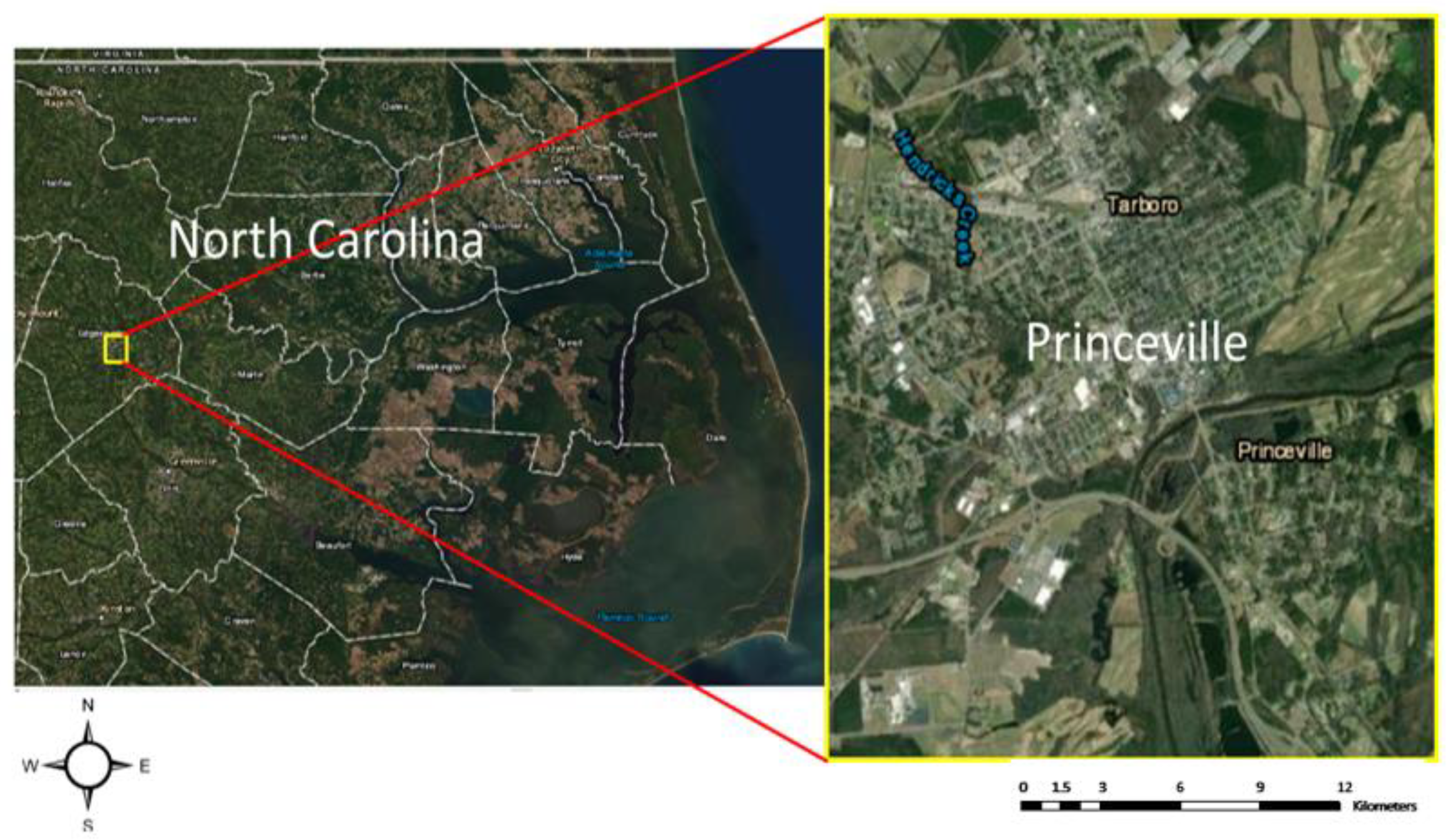
2. Study Area and Data
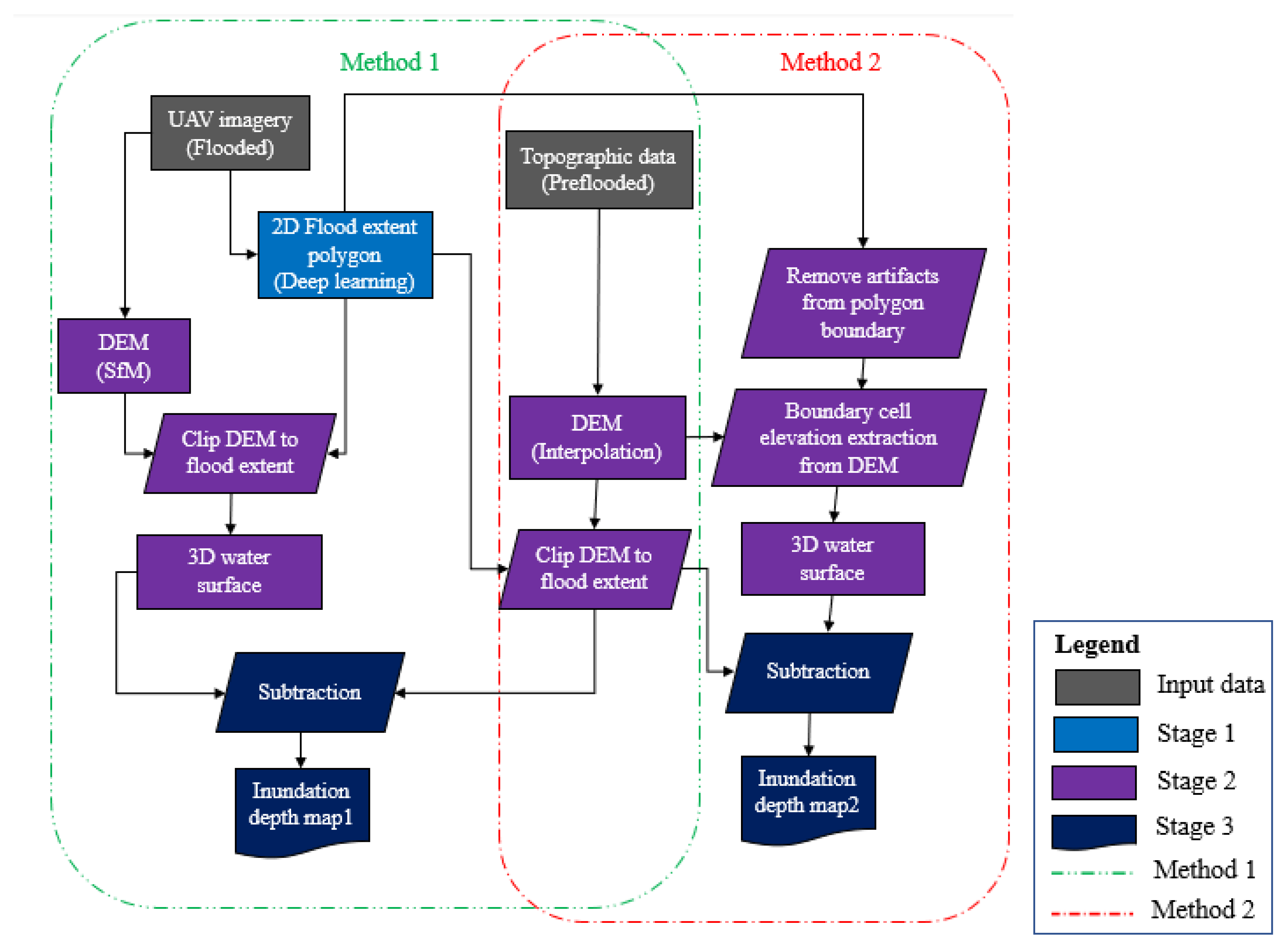
The town of Princeville, a flood-prone area in North Carolina in the USA, was selected as our study area for this research (Figure 1). Princeville is located along the Tar River in Edgecombe County and has been seriously affected by several flood events, including Hurricane Floyd and Hurricane Matthew. They both caused widespread devastation when the Tar river overflowed.
The datasets used for the study include UAV imagery and Lidar data, which were acquired by North Carolina Emergency Management. The flood imagery in Princeville was collected during Hurricane Matthew in 2016 using a Trimble UX5 fixed-wing UAV. Each image consisted of three bands (RGB) at 2.6 cm spatial resolution. The LiDAR data was acquired in 2014 with two pulses per square meter (pls/m2) with an accuracy of 9.25 cm RMSE and was used to generate a pre-flood DEM over the town of Princeville. We also collected USGS surface water gauge station information on the study area from the NOAA website. USGS gauge stations collect time-series data that describe stream levels, streamflow or discharge, reservoir and lake levels, surface-water quality, and rainfall.

3. Methodology

In this section, the two proposed methods for estimating flood depths are discussed. The workflow for the methods is shown in Figure 2. The proposed approaches involve three stages: (1) 2D inundation mapping; (2) 3D water surface generation; and (3) floodwater depth estimation.

3.1. Stage 1: Flood Extent Mapping

The first stage of the methods involved automatically extracting the flood extent from imagery data (e.g., UAV data). The flood extent mapping in this study was based on the authors’ approach [18], which fine-tuned a fully convolutional neural network with a stride of 8 (FCN-8s) model. The FCN-8s was proposed by Long et al. [37] to train an end-to-end directly from the input images for semantic segmentation. In this model, VGG16 fully-connected-based classification layers [38] were replaced by convolutional layers to maintain the 2D structure of images. The data processing based on this method consisted of training, testing, and evaluation stages. In the training stage, the network trained using 150 manually annotated UAV images (4000 x 4000-pixel size each) using stochastic gradient descent (SGD) for 6 epochs with a learning rate of 0.001, and a maximum batch size of 2. The Hurricane Matthew UAV images acquired in the city of Lumberton in 2016 were used to train the FCN-8s model, whereas the Hurricane Florence image collected over the city of Princeville was used to test the model. The results were then georeferenced using 8 GCPs available in the study area for geospatial data integration purposes, since the training and testing images were not georeferenced initially. In the accuracy assessment stage, the confusion matrix was calculated to analyze the performance of the FCN-8s. Finally, the FCN-based extent map was converted to inundation polygons using raster to vector conversion for further spatial data analysis, integration, and visualization. More detailed information about the floodwater extent mapping approach can be found in [18].

3.2. Stage 2: Creating 3D Water Surface

3.2.1. Method 1: 3D Water Surface Reconstruction using SfM and CNN

In this approach, SFM was used to create a 3D point cloud or 3D digital surface model of the study area from UAV imagery data. SfM is a photogrammetry method to reconstruct a 3D point cloud from a series of overlapped 2D photos of an area or an object taken from different angles [39]. SFM employs feature-based image matching methods such as scale-invariant feature transform (SIFT) to automatically identify matching features in these input photos. The features are tracked from photo to photo and are used to estimate the camera positions and orientations and the features’ coordinates, and finally, create a 3D point cloud for features.
The point cloud created using the SfM approach is unclassified; 3D point cloud classification is a crucial step to group water points, reconstruct 3D water surface, and extract meaningful information from the inundation areas. However, the classification is very challenging due to irregular geometric attributes and highly noisy and nonuniform sampling of point cloud data. To overcome the issue of point cloud classification, we proposed to employ the flood extent polygons created using the deep learning method in stage 1 and spatial overlay analysis to classify the point cloud to water (water/flood) and no water (dry) points. Then, a noise removal method needed to be implemented to identify and eliminate noise points and obvious outliers that do not represent the actual water surface from the water point’s class. The noise removal stage is very critical, as generating point clouds using photogrammetry containing water bodies tends to be problematic due to the homogeneous appearance of the water surface and insufficient tie-points for image matching and create noise points above and below the water surface. The issues are especially troublesome as they adversely affect the water surface estimation and consequently result in underestimating or overestimating water depth measurements. We used a hydro-flattened approach to enhance the water point cloud surface by removing artifacts, considering the water bodies to be flat bank to bank with a constant elevation within each bank/polygon. Finally, the point cloud interpolation was done to create water surfaces (flood DEM) with a 10 cm cell size.

3.2.2. Method 2: 3D Water Reconstruction using DEM and CNN

This research also investigated another method to create a 3D water surface by spatial analysis of the flood extent extracted using the deep learning method and pre-flood DEM elevation. In this approach, 3D water surfaces were obtained by intersecting the flood extent polygons and the DEM and creating 3D water/dry interfaces. Thus, the elevation of each inundation area’s boundary was computed by performing a statistical analysis of their elevation values from the DEM. This approach assumes that the water surface of the flooded areas is flat and has constant water elevation inside each detected flood/water polygon. It should be noted that the assumption of a constant water surface elevation across individual polygons may not completely accurate for extreme events due to complex flow paths. It should be also noted that the elevation of the polygon vertices on the water–vegetation or water–building interfaces should be modified, as there is an ambiguity in the water level estimation in those areas. In other words, the line segments resulting from the intersection of water and vegetation polygons or water and building polygons do not necessarily represent the interfaces between dry and water areas [40,41]. Thus, assigning a water elevation to any point located on those line segments could be inaccurate. In the research, our algorithm assigned the mean water elevation of the polygon vertices located on water/dry interfaces to these line segments and finally created a 3D water surface/mask for the area. In this study, water surface and pre-flood DEM were created with 10 cm cell sizes to match with the water surface (flood DEM) previously created in Section 3.2.1 for pixel by pixel floodwater comparison purposes. Although this method is fast and straightforward, the 3D water surface quality heavily relies on the quality of DEM and floodwater extent.

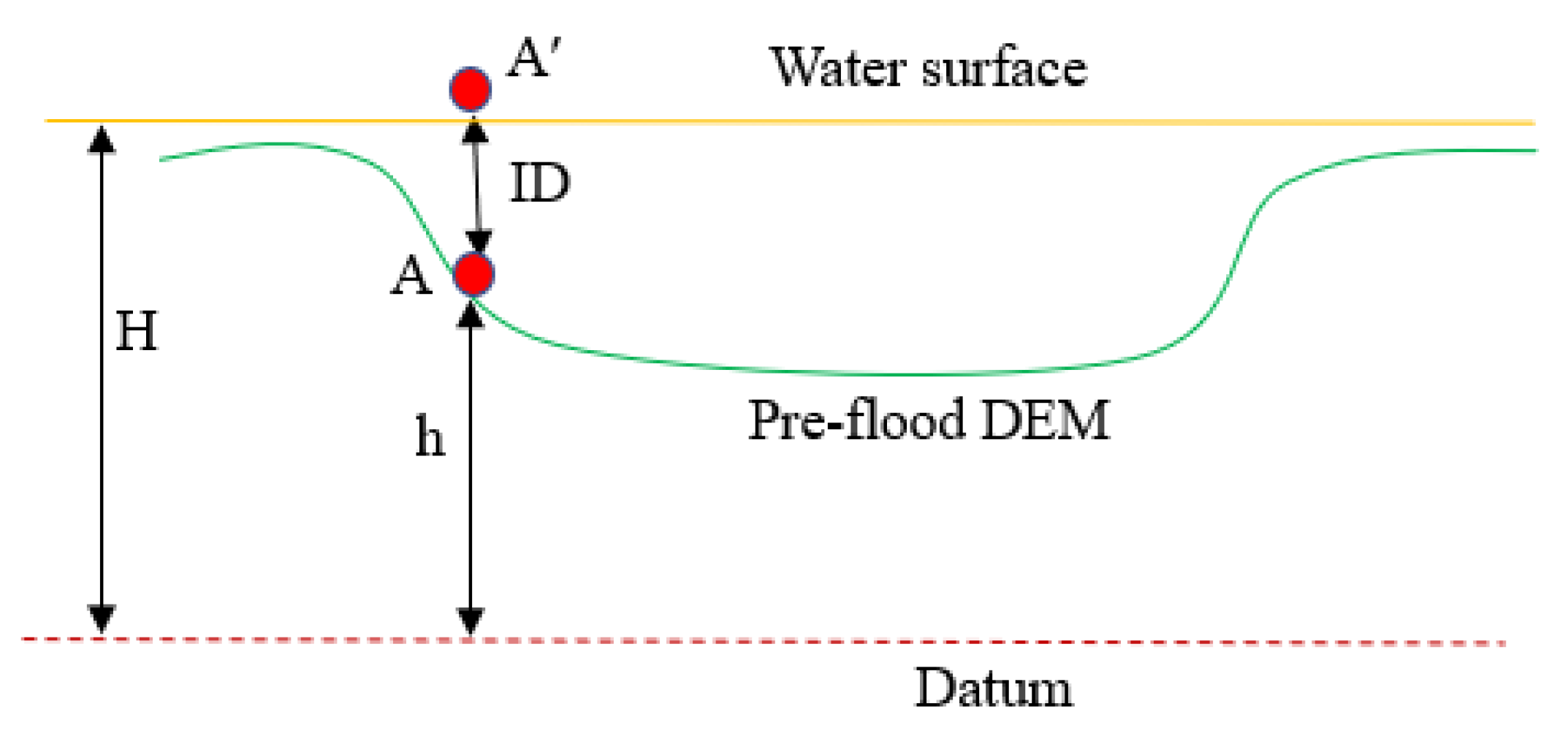
3.3. Stage 3: Floodwater Depth Estimation

In Stage 2, 3D water surfaces were created using two different methods. The inundation depth could simply be estimated for each pixel as the difference between the pre-flood DEM and the 3D water surfaces created in stage 2 (Figure 3).
Figure 3 represents a cross-section of a 3D water surface or mask (yellow line) and a cross-section of the pre-flood DEM and datum that are shown by green profile and red dashed line, respectively. H is the elevation of the water surface above the datum, h is the elevation of the earth’s surface before the flood event, and ID is the inundation depth. Assume A is a point (pixel) on the earth’s surface and A′ is the location of the corresponding point on the water surface (inundation area). The pre-flood DEM is considered as a benchmark to estimate the floodwater depth. The elevation difference between the 3D water surface (H) and its corresponding pixel point on the DEM (h) gives the inundation depth (ID):
ID = H − h

3.4. Evaluation and Comparison

The proposed approach’s performance was evaluated using the gauge station elevation obtained from the USGS website. The root mean squared error (RMSE) assessment technique was used to quantify the floodwater depth error calculated using the proposed methods. RMSE is used to measure how well a given model performs. Two RMSEs were calculated to quantify the floodwater depth error calculated using our two proposed methods: a) SfM and deep learning classification, and b) deep learning, DEM, and spatial analysis. Based on the RMSE results, the two methods’ performance were compared, and a conclusion was made.

4. Implementation

The methodology for flood extent mapping and water depth measurements was implemented using MATLAB, Pix4Dmapper, and ArcGIS. The computing unit was configured with 32 GB memory, an Intel(R) Xeon(R) ES-2620 v3 @ 2.40GHz ×2 processors memory, and a single NVIDIA Quadro M4000 GPU.

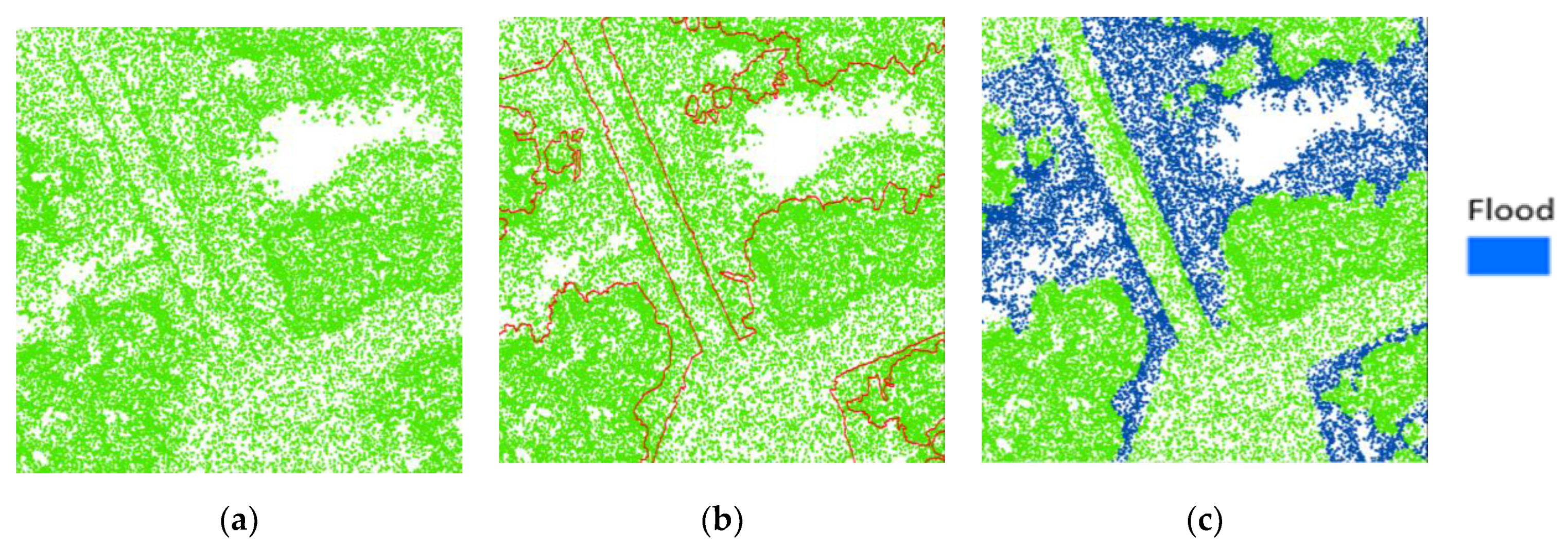
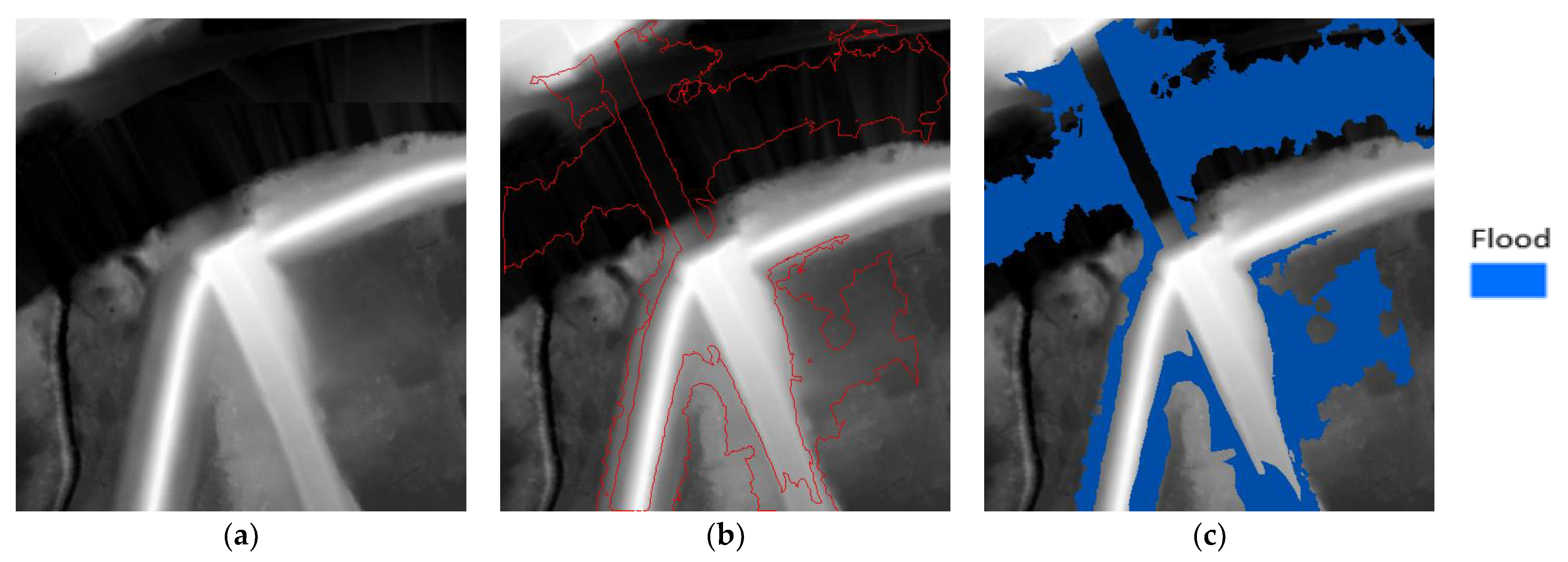
4.1. Flood Extent Mapping Results

The UAV images were classified using FCN-8s to extract the flood extent map. Figure 4 illustrates the classification results (water, building, vegetation, and others), and the detailed information on the performance of each classifier is described via the confusion matrix in Table 1. As previously mentioned, vegetation and building polygons were needed to modify the 3D water surface (3D inundation map) at building–water and vegetation–water interfaces. The overall accuracy and kappa index achieved by FCN-8s were about 97% and 0.934, respectively.
For more detailed information on the implementation of stage 1 (deep learning image classification) please see [18]. Our primary goal was to extract inundation areas (water class) from the UAV imagery. The FCN-8s achieved 98.71% accuracy in extracting the inundation areas in non-vegetated areas from the UAV imagery. Having an accurate flood extent map is vital for floodwater depth measurements based on the proposed approaches, because the flood extent map leads the classification of the SFM-based point cloud (method 1) and spatial analysis/overlay (method 2).

4.2. 3D Water Surface Reconstruction

4.2.1. Method 1: 3D Water Surface using SfM and CNN

Figure 5 shows the 3D water point classification and water surface creation results using SfM and CNN methods. A total of 1800 UAV images with 4000 × 4000 pixels size and 80% overlap between consecutive images were processed for 3D point cloud generation using the SFM method. Four ground control points (GCPs) within our study area were used for georeferencing. Note that acquiring remote sensing images using the Real-Time Kinematic Global Navigation Satellite System (RTK-GNSS)-mounted UAV or post-processing kinematic (PPK) technology can reduce the use of GCPs for georeferencing purposes in the photogrammetry process. The use of RTK or PPK helps to avoid time-consuming target deployment procedures and provides the position of each image with centimeter-scale accuracy [42]. The point cloud resulting from SfM was unclassified; thus, the flood extent polygons were overlaid on the 3D point cloud to identify the point data within the inundation areas (Figure 5b) and classify the point clouds as flood and non-flood points (Figure 5c). The quality of 3D flood point data was improved using a noise removal process, and then a 3D water surface was created using the natural neighbor interpolation technique. Voids in the point cloud occurred in some inundation areas where the selection of sufficient tie-points to reference the UAV images was challenging due to the water surface’s homogenous appearance. This may have affected the depth estimation in those areas, since the elevation of the void areas was estimated by interpolation of nearby point clouds.

4.2.2. Method 2: 3D Water Surface using DEM and CNN

Figure 6 shows the 3D water surface created using DEM and CNN (method 2). A LiDAR-based DEM was created to represent the pre-flood elevation model of the study area (Figure 6a). This DEM was created with a 10 cm cell size to match the SfM-based pre-flood DEM for pixel-based computation. The LiDAR data was acquired by North Carolina Emergency Management using a linear aerial sensor, collected at 2 points per meter in 2014. The 3D water surface was created by intersecting the water polygons extracted by CNN and the pre-flood DEM and extracting the water elevation (z) for the water polygons boundaries from DEM (Figure 6b) with the assumption that inundation areas have a constant water elevation within each water polygon.

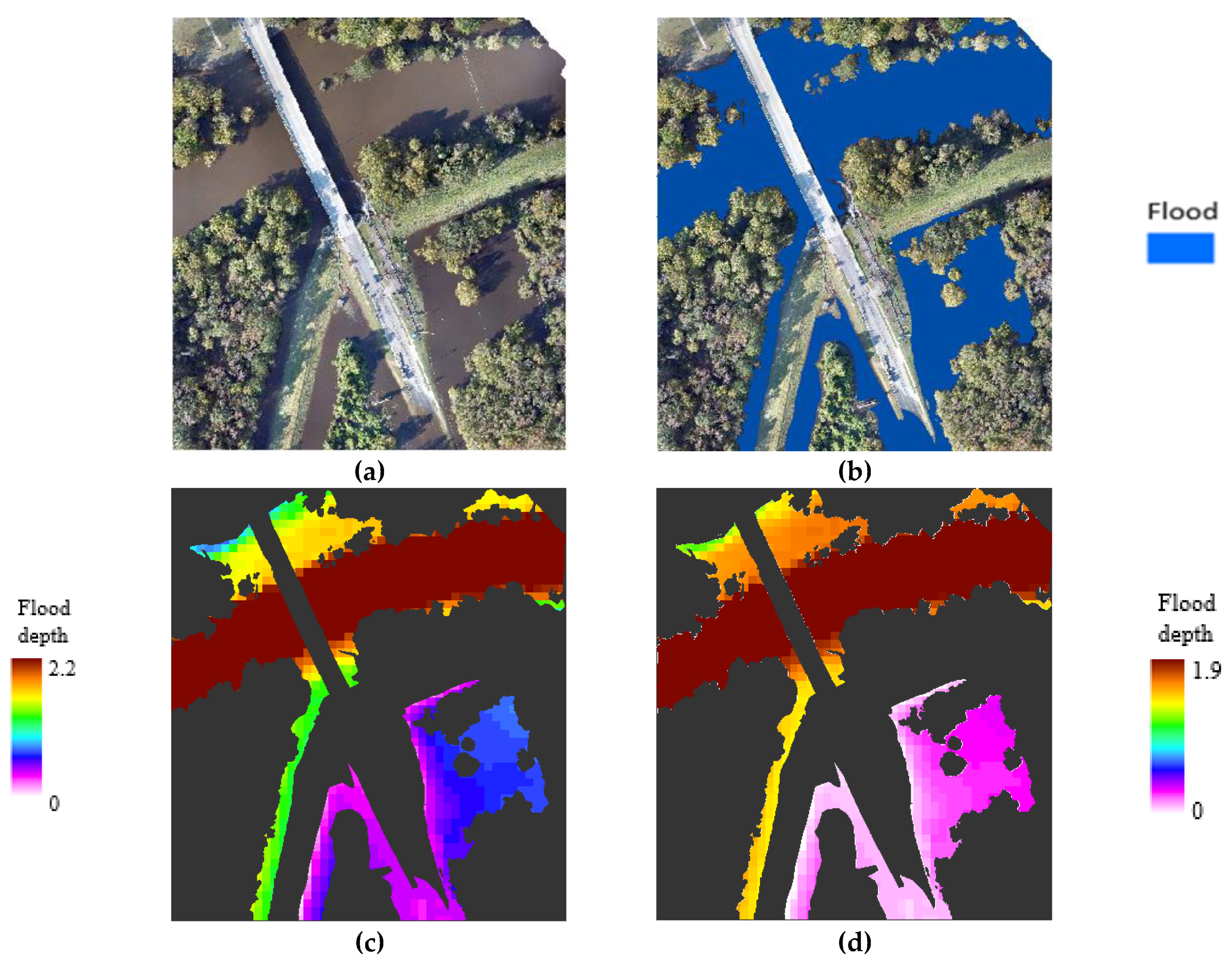
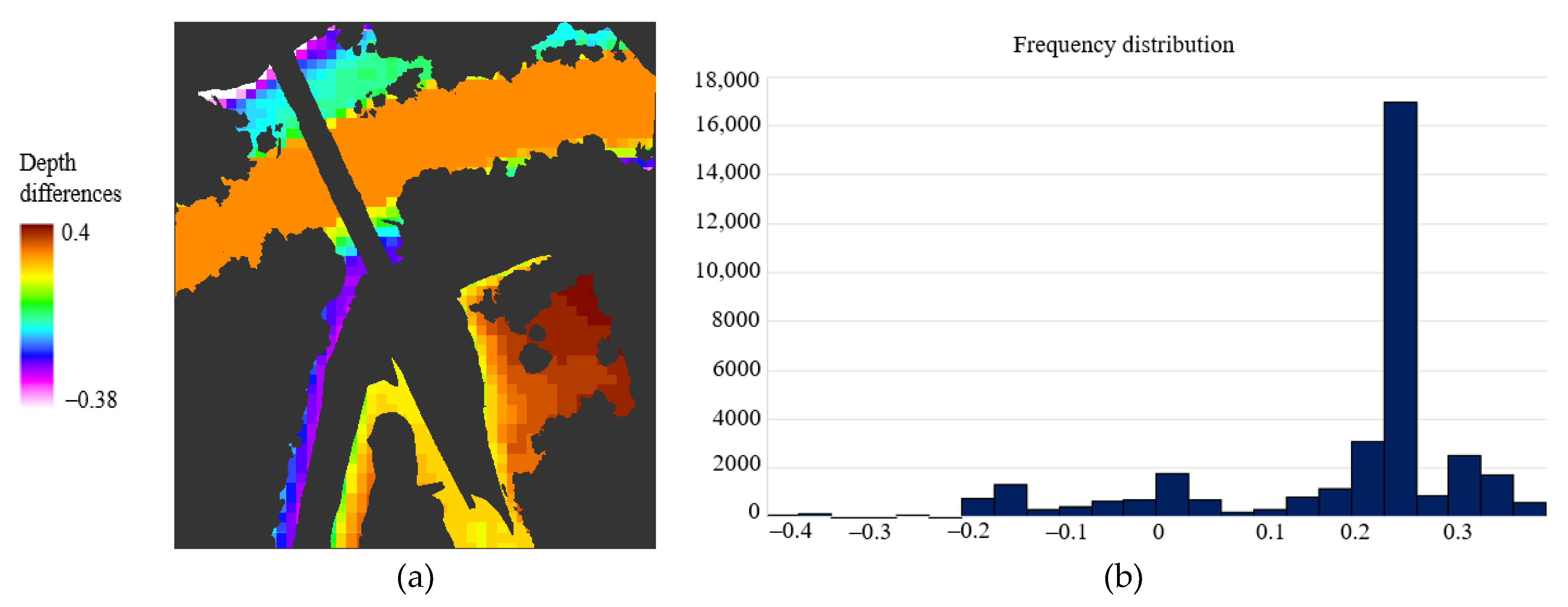
4.3. Floodwater Depth Estimation Results

Figure 7 shows the inundation depth (ID) results for the water surfaces created by two proposed methods for the study area. Figure 7b illustrates the 2D inundation map created for the test image (Figure 7a) using FCN-8s. The results show the FCN-8s accurately extracted the flood extent from the test UAV image. The IDs were estimated by subtracting water surface raster data (stage 2) and pre-flood DEM. Floodwater depth estimates by method 1 (SfM and CNN) and method 2 (DEM and CNN) are illustrated in Figure 7c,d, respectively. The maximum water depths measured using method 1 and method 2 were 1.86 m and 2.2 m, respectively; these depth values for both approaches were recorded in the river area, as shown in Figure 7c,d (red areas). The areas with zero water depth or dry areas are shown in black.
The inundation depth maps were compared to determine how the spatial distribution of water depth measurements are correlated. The floodwater depth rasters were compared cell-by-cell, and a water depth difference surface was created (Figure 8a). Figure 8b shows the histogram of flood depth differences between the two approaches. The maximum and minimum absolute flood depth differences were 0.4 m and 0.001 m, respectively. The mean difference value was 0.2 m with a standard deviation of 0.1 m. The performance of the methods was also evaluated by comparing the IDs against the water gauge data. The RMSEs measured for method 1 and method 2 using the gauge elevation data were 0.34 m and 0.26 m, respectively. Based on the research results, method 2 offers better estimation performance compared to method 1.
Two main factors affecting the quality and performance of the methods for inundation depth estimation include a) the DEM quality, and b) the inundation extent map quality.
  • DEM quality. Accurate topography data or DEM is indispensable for various remote sensing applications, including flood mapping. The DEM generation methods, such as LiDAR or photogrammetry, yield different levels of accuracy. LiDAR is generally the preferred source for generating elevation data due to its high data quality and ability to map beneath the canopy. For this research, we used two types of DEM: pre-flood LiDAR, and (photogrammetric) SFM-based DEM. Method 1 used these two DEMs to estimate floodwater depths. Method 2, on the other hand, only used pre-flood LiDAR-based DEM and spatial analysis to calculate floodwater depth.
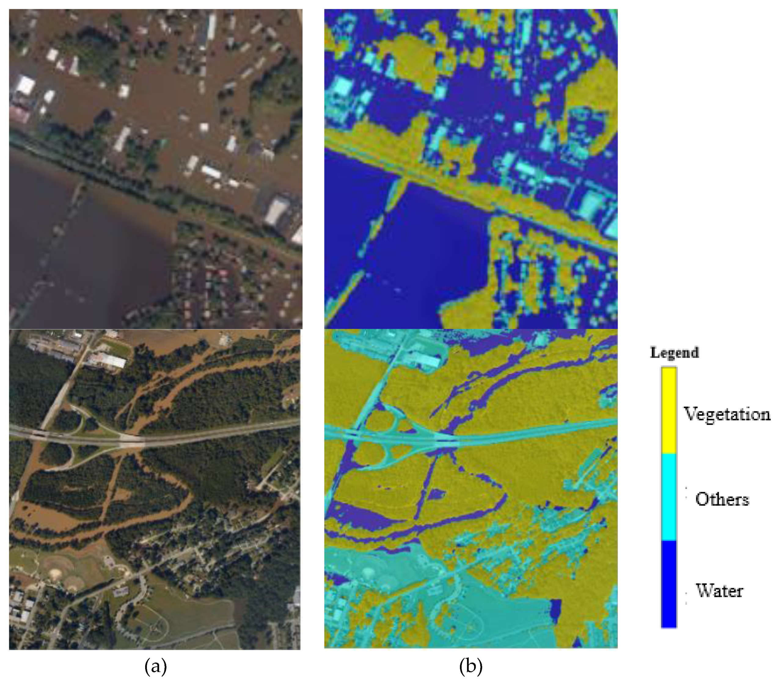
  • Inundation extent map quality. The flood extent map accuracy is also another factor that affects the floodwater depth estimation approach’s performance, because the 3D point cloud classification in method 1 and the water elevation extraction in method 2 highly depend on the flood extent polygon planimetric accuracy. Both methods use the flood extent polygon as input for inundation depth estimations. One of the advantages of the proposed approaches is using deep learning-based flood extent polygons. The data-driven and deep learning methods like FCN8s have been proven to be efficient for classification tasks and achieved promising results (with 98.7% accuracy) in extracting flooded areas, reducing the issue of overestimation or underestimating floodwater depths.
Overall, using accurate flood extent and DEM can improve the performance of the methods for flood depth estimations. The estimated floodwater depth values give additional information that can be used for rescue and damage assessment tasks.

5. Conclusions

The research proposes two approaches to calculate inundation depth using photogrammetric and topographic data. The proposed approaches calculate inundation depth information based on the integration of 3D flood extent and a DEM. These methods are only different in how they reconstruct their 3D water surface. The first approach used SfM to create a 3D point cloud for the area, and the water polygons were applied for water point cloud classification. In contrast, the second method reconstructed the water surface by intersecting the water polygons (2D flood extent) and a pre-flood DEM. The deep learning segmentation method used for 2D inundation mapping allowed for precise and rapid floodwater depth estimation, which is highly advantageous for immediate emergency response and damage assessments. The methods were compared and validated using the USGS gauge water level data acquired during the flood event and demonstrated promising results. The RMSEs measured for method 1 and method 2 were 0.34 m and 0.26 m, respectively. These results reveal that deep learning-based flood extent polygon (with 98.7% accuracy) is a promising method to classify the SFM floodwater point cloud and create a 3D water surface, which is a crucial step for water depth estimation. Future work will focus on further validation and comparison of the proposed methods using more in situ data in different study areas, and it will study the effects of image resolution and DEM quality in 3D inundation mapping.

Author Contributions

Conceptualization, Leila Hashemi-Beni and Asmamaw A Gebrehiwot; methodology, Leila Hashemi-Beni and Asmamaw A Gebrehiwot; software, Asmamaw A Gebrehiwot and Leila Hashemi-Beni; validation, Asmamaw A Gebrehiwot, Leila Hashemi-Beni; investigation, Leila Hashemi-Beni and Asmamaw A Gebrehiwot; resources, Leila Hashemi-Beni; data curation, Asmamaw A Gebrehiwot; writing—original draft preparation, Asmamaw A Gebrehiwot and Leila Hashemi-Beni; writing—review and editing, Leila Hashemi-Beni and Asmamaw A Gebrehiwot; visualization, Asmamaw A Gebrehiwot and Leila Hashemi-Beni; supervision, Leila Hashemi-Beni; project administration, Leila Hashemi-Beni; funding acquisition, Leila Hashemi-Beni All authors have read and agreed to the published version of the manuscript.

Funding

This research was funded by the U.S. National Science Foundation (NSF), grant number 1800768, and North Carolina Collaboratory Policy.

Institutional Review Board Statement

Not applicable.

Informed Consent Statement

Not applicable.

Data Availability Statement

Data sharing not applicable.

Acknowledgments

The authors would like to thank the North Carolina Emergency Management for providing the UAV and LiDAR data, GCPs, and support data for the project.

Conflicts of Interest

The authors declare no conflict of interest.

References

  1. Rodriguez, J.; Vos, F.; Below, R.; Guha-Sapir, D. Annual Disaster Statistical Review 2008. In The Numbers and Trends; Centre for Research on the Epidemiology of Disasters (CRED): Brussels, Belgium, 2009. [Google Scholar]
  2. Best Practices in Disaster Recovery—Before the Storm. Available online: https://www.texastribune.org/2018/01/08/hurricane-harvey-was-years-costliest-us-disaster-125-billion-damages/ (accessed on 7 August 2018).
  3. Hurricane Harvey: Facts, FAQs, and how to help, World Vision. 2017. Available online: https://www.worldvision.org/disaster-relief-news-stories/2017-hurricane-harvey-facts (accessed on 7 September 2018).
  4. 2017′s three monster hurricanes—Harvey, Irma, and Maria—Among five costliest ever, US Today. Available online: https://www.usatoday.com/story/weather/2018/01/30/2017-s-three-monster-hurricanes-harvey-irma-and-maria-among-five-costliest-ever/1078930001/ (accessed on 1 February 2018).
  5. Borowska-Stefańska, M.; Kowalski, M.; Wiśniewski, S. The Measurement of Mobility-Based Accessibility—The Impact of Floods on Trips of Various Length and Motivation. ISPRS Int. J. Geo-Inf. 2019, 8, 534. [Google Scholar] [CrossRef] [Green Version]
  6. Beni, L.H.; Mostafavi, M.A.; Pouliot, J. 3D dynamic simulation within GIS in support of disaster management. In Geomatics Solutions for Disaster Management; Springer: Berlin/Heidelberg, Germany, 2007; pp. 165–184. [Google Scholar]
  7. Sheffield, J.; Wood, E.F.; Pan, M.; Beck, H.; Coccia, G.; Serrat-Capdevila, A.; Verbist, K. Satellite remote sensing for water resources management: Potential for supporting sustainable development in data-poor regions. Water Resour. Res. 2018, 54, 9724–9758. [Google Scholar] [CrossRef] [Green Version]
  8. Hashemi-Beni, L.; Gebrehiwot, A. Deep Learning for Remote Sensing Image Classification for Agriculture Applications. Int. Arch. Photogramm. Remote Sens. Spat. Inf. Sci. 2020, 44, 51–54. [Google Scholar] [CrossRef]
  9. Revilla-Romero, B.; Hirpa, F.A.; Pozo, J.T.D.; Salamon, P.; Brakenridge, R.; Pappenberger, F.; De Groeve, T. On the use of global flood forecasts and satellite-derived inundation maps for flood monitoring in data-sparse regions. Remote Sens. 2015, 7, 15702–15728. [Google Scholar] [CrossRef] [Green Version]
  10. Pradhan, B.; Tehrany, M.S.; Jebur, M.N. A new semiautomated detection mapping of flood extent from TerraSAR-X satellite image using rule-based classification and taguchi optimization techniques. IEEE Trans. Geosci. Remote Sens. 2016, 54, 4331–4342. [Google Scholar] [CrossRef]
  11. Wang, D.; Wan, B.; Qiu, P.; Su, Y.; Guo, Q.; Wang, R.; Wu, X. Evaluating the performance of sentinel-2, landsat 8 and pléiades-1 in mapping mangrove extent and species. Remote Sens. 2018, 10, 1468. [Google Scholar] [CrossRef] [Green Version]
  12. Boccardo, P.; Chiabrando, F.; Dutto, F.; Tonolo, F.; Lingua, A. UAV deployment exercise for mapping purposes: Evaluation of emergency response applications. Sensors 2015, 15, 15717–15737. [Google Scholar] [CrossRef] [Green Version]
  13. Gao, B.C. NDWI—A normalized difference water index for remote sensing of vegetation liquid water from space. Remote Sens. Environ. 1996, 58, 257–266. [Google Scholar] [CrossRef]
  14. Long, S.; Fatoyinbo, T.E.; Policelli, F. Flood extent mapping for Namibia using change detection and thresholding with SAR. Environ. Res. Lett. 2014, 9, 035002. [Google Scholar] [CrossRef]
  15. Feng, Q.; Liu, J.; Gong, J. Urban flood mapping based on unmanned aerial vehicle remote sensing and random forest classifier—A case of Yuyao, China. Water 2015, 7, 1437–1455. [Google Scholar] [CrossRef]
  16. Nandi, I.; Srivastava, P.; Shah, K. Floodplain mapping through support vector machine and optical/infrared images from Landsat 8 OLI/TIRS sensors: Case study from Varanasi. Water Resour. Manag. 2017, 31, 1157–1171. [Google Scholar] [CrossRef]
  17. Gebrehiwot, A.; Hashemi-Beni, L. A Method to Generate Flood Maps in 3d Using dem and Deep Learning. Int. Arch. Photogramm. Remote Sens. Spat. Inf. Sci. 2020, 44, 25–28. [Google Scholar] [CrossRef]
  18. Gebrehiwot, A.; Hashemi-Beni, L.; Thompson, G.; Kordjamshidi, P.; Langan, T.E. Deep convolutional neural network for flood extent mapping using unmanned aerial vehicle data. Sensors 2019, 19, 1486. [Google Scholar] [CrossRef] [Green Version]
  19. Peng, B.; Liu, X.; Meng, Z.; Huang, Q. Urban flood mapping with residual patch similarity learning. In Proceedings of the 3rd ACM SIGSPATIAL International Workshop on AI for Geographic Knowledge Discovery, Seattle, WA, USA, 5 November 2019; pp. 40–47. [Google Scholar]
  20. Sarker, C.; Mejias, L.; Maire, F.; Woodley, A. Flood mapping with convolutional neural networks using spatio-contextual pixel information. Remote Sens. 2019, 11, 2331. [Google Scholar] [CrossRef] [Green Version]
  21. Wu, C.; Yang, X.; Wang, J. Flood Detection in Sar Images Based on Multi-Depth Flood Detection Convolutional Neural Network. In Proceedings of the 2019 IEEE 6th Asia-Pacific Conference on Synthetic Aperture Radar (APSAR 2019), Xiamen, China, 26–29 November 2019; pp. 1–6. [Google Scholar]
  22. Kang, W.; Xiang, Y.; Wang, F.; Wan, L.; You, H. Flood detection in gaofen-3 SAR images via fully convolutional networks. Sensors 2018, 18, 2915. [Google Scholar] [CrossRef] [PubMed] [Green Version]
  23. Jarihani, A.A.; Callow, J.N.; Johansen, K.; Gouweleeuw, B. Evaluation of multiple satellite altimetry data for studying inland water bodies and river floods. J. Hydrol. 2013, 505, 78–90. [Google Scholar] [CrossRef]
  24. Baup, F.; Frappart, F.; Maubant, J. Combining high-resolution satellite images and altimetry to estimate the volume of small lakes. Hydrol. Earth Syst. Sci. 2014, 18, 2007–2020. [Google Scholar] [CrossRef] [Green Version]
  25. Ovando, A.; Martinez, J.M.; Tomasella, J.; Rodriguez, D.A.; von Randow, C. Multi-temporal flood mapping and satellite altimetry used to evaluate the flood dynamics of the Bolivian Amazon wetlands. Int. J. Appl. Earth Obs. Geoinf. 2018, 69, 27–40. [Google Scholar] [CrossRef]
  26. Meesuk, V.; Vojinovic, Z.; Mynett, A.E. Using multidimensional views of photographs for flood modeling. In Proceedings of the 2012 IEEE 6th International Conference on Information and Automation for Sustainability, Beijing, China, 27–29 September 2012; pp. 19–24. [Google Scholar]
  27. Meesuk, V.; Vojinovic, Z.; Mynett, A.E.; Abdullah, A.F. Urban flood modeling combining top-view LiDAR data with ground-view SfM observations. Adv. Water Resour. 2015, 75, 105–117. [Google Scholar] [CrossRef]
  28. Hashemi-Beni, L.; Jones, J.; Thompson, G.; Johnson, C.; Gebrehiwot, A. Challenges and opportunities for UAV-based digital elevation model generation for flood-risk management: A case of Princeville, North Carolina. Sensors 2018, 18, 3843. [Google Scholar] [CrossRef] [PubMed] [Green Version]
  29. Schumann, G.; Hostache, R.; Puech, C.; Hoffmann, L.; Matgen, P.; Pappenberger, F.; Pfister, L. High-resolution 3-D flood information from radar imagery for flood hazard management. IEEE Trans. Geosci. Remote Sens. 2007, 45, 1715–1725. [Google Scholar] [CrossRef]
  30. Matgen, P.; Schumann, G.; Henry, J.B.; Hoffmann, L.; Pfister, L. Integration of SAR-derived river inundation areas, high-precision topographic data and a river flow model toward near real-time flood management. Int. J. Appl. Earth Obs. Geoinf. 2007, 9, 247–263. [Google Scholar] [CrossRef]
  31. Huang, C.; Chen, Y.; Wu, J.; Chen, Z.; Li, L.; Liu, R.; Yu, J. Integration of remotely sensed inundation extent and high-precision topographic data for mapping inundation depth. In Proceedings of the 2014 IEEE 3rd International Conference on Agro-Geoinformatics, Beijing, China, 11–14 August 2014; pp. 1–4. [Google Scholar]
  32. Cian, F.; Marconcini, M.; Ceccato, P.; Giupponi, C. Flood depth estimation by means of high-resolution SAR images and lidar data. Nat. Hazards Earth Syst. Sci. 2018, 18, 3063–3084. [Google Scholar] [CrossRef] [Green Version]
  33. Manfreda, S.; Samela, C. A digital elevation model-based method for a rapid estimation of flood inundation depth. J. Flood Risk Manag. 2019, 12, e12541. [Google Scholar] [CrossRef] [Green Version]
  34. Lou, H.; Wang, P.; Yang, S.; Hao, F.; Ren, X.; Wang, Y.; Shi, L.; Wang, J.; Gong, T. Combining and comparing an unmanned aerial vehicle and multiple remote sensing satellites to calculate long-term river discharge in an ungauged water source region on the Tibetan Plateau. Remote Sens. 2020, 12, 2155. [Google Scholar] [CrossRef]
  35. Yang, S.; Wang, P.; Lou, H.; Wang, J.; Zhao, C.; Gong, T. Estimating river discharges in ungauged catchments using the slope–area method and unmanned aerial vehicle. Water 2019, 11, 2361. [Google Scholar] [CrossRef] [Green Version]
  36. Zazo, S.; Molina, J.L.; Rodríguez-Gonzálvez, P. Analysis of flood modeling through innovative geomatic methods. J. Hydrol. 2015, 524, 522–537. [Google Scholar] [CrossRef]
  37. Long, J.; Shelhamer, E.; Darrell, T. Fully convolutional networks for semantic segmentation. In Proceedings of the 2015 IEEE Conference on Computer Vision and Pattern Recognition, Boston, MA, USA, 7–12 June 2015; pp. 3431–3440. [Google Scholar]
  38. Simonyan, K.; Zisserman, A. Very deep convolutional networks for large-scale image recognition. arXiv 2014, arXiv:1409.1556. [Google Scholar]
  39. Turner, D.; Lucieer, A.; Watson, C. An automated technique for generating georectified mosaics from ultra-high resolution unmanned aerial vehicle (UAV) imagery, based on structure from motion (SfM) point clouds. Remote Sens. 2012, 4, 1392–1410. [Google Scholar] [CrossRef] [Green Version]
  40. Gebrehiwot, A.; Hashemi-Beni, L. Automated Indunation Mapping: Comparison of Methods. In Proceedings of the IGARSS 2020-2020 IEEE International Geoscience and Remote Sensing Symposium, Virtual, 26 September–2 October 2020; pp. 3265–3268. [Google Scholar]
  41. Hashemi-Beni, L.; Gebrehiwot, A. Flood Extent Mapping: An Integrated Method using Deep Learning and Region Growing Using UAV Optical Data. IEEE J. Sel. Top. Appl. Earth Obs. Remote Sens. 2021, 14, 2127–2135. [Google Scholar] [CrossRef]
  42. Forlani, G.; Dall’Asta, E.; Diotri, F.; Cella, U.M.D.; Roncella, R.; Santise, M. Quality assessment of DSMs produced from UAV flights georeferenced with on-board RTK positioning. Remote Sens. 2018, 10, 311. [Google Scholar] [CrossRef] [Green Version]
Figure 1. Study area—Princeville, North Carolina.
Ijgi 10 00144 g001
Figure 2. The proposed methods for floodwater depth estimation.
Ijgi 10 00144 g002
Figure 3. A schematic description of inundation depth estimation.
Ijgi 10 00144 g003
Figure 4. Two sample FCN-8s) results. (a) Input aircraft images acquired during Hurricane Matthew in Lumberton, NC in Oct 2016; (b) classification results.
Ijgi 10 00144 g004
Figure 5. Three-dimensional surface reconstruction using method 1. (a) SfM-based unclassified point cloud; (b) overlaying flood extent polygons (red polygons) on the point cloud; (c) 3D point cloud classification for flood and non-flood point data. Note: the figures show a small portion of the study area (clipped) for the sake of visualization of the dense point cloud.
Ijgi 10 00144 g005
Figure 6. Three-dimensional surface reconstruction using DEM and CNN; (a) pre-flood DEM; (b) intersecting flood extent polygons (red polygons) and DEM and extract Z value for each polygon; (c) 3D water surface (raster format).
Ijgi 10 00144 g006
Figure 7. Inundation depths results; (a) test image; (b) flood extent from CNN; (c) ID results for method 1; (d) ID results for method 2.
Ijgi 10 00144 g007
Figure 8. Floodwater depth comparison. (a) Water depth difference between method 2 and method 1; (b) a histogram that shows frequencies distributions of the flood depth difference between the two methods.
Ijgi 10 00144 g008
Table 1. Confusion matrix of FCN-8s (unit: percentage).
WaterOthersVegetation
water98.710.850.44
others1.5195.522.97
vegetationdata1.3198.43
Publisher’s Note: MDPI stays neutral with regard to jurisdictional claims in published maps and institutional affiliations.

