Machine Learning-Based Processing Proof-of-Concept Pipeline for Semi-Automatic Sentinel-2 Imagery Download, Cloudiness Filtering, Classifications, and Updates of Open Land Use/Land Cover Datasets

Abstract

Land use and land cover are continuously changing in today’s world. Both domains, therefore, have to rely on updates of external information sources from which the relevant land use/land cover (classification) is extracted. Satellite images are frequent candidates due to their temporal and spatial resolution. On the contrary, the extraction of relevant land use/land cover information is demanding in terms of knowledge base and time. The presented approach offers a proof-of-concept machine-learning pipeline that takes care of the entire complex process in the following manner. The relevant Sentinel-2 images are obtained through the pipeline. Later, cloud masking is performed, including the linear interpolation of merged-feature time frames. Subsequently, four-dimensional arrays are created with all potential training data to become a basis for estimators from the scikit-learn library; the LightGBM estimator is then used. Finally, the classified content is applied to the open land use and open land cover databases. The verification of the provided experiment was conducted against detailed cadastral data, to which Shannon’s entropy was applied since the number of cadaster information classes was naturally consistent. The experiment showed a good overall accuracy (OA) of 85.9%. It yielded a classified land use/land cover map of the study area consisting of 7188 km2 in the southern part of the South Moravian Region in the Czech Republic. The developed proof-of-concept machine-learning pipeline is replicable to any other area of interest so far as the requirements for input data are met.

1. Introduction

Land use and land cover are commonly used as synonyms and are often merged into a single dataset. The abbreviation LULC (land use/land cover) is used for this concept. Nevertheless, land use and land cover refer to different phenomena. In part, we can view land use as an extension of land cover, considering that it describes human activities, most of which being firmly bound to a certain surface type (land cover type).

Fisher, Comber, and Wadsworth [1] argued that the advent of remote sensing (RS) in the 1970s caused a shift in the perception of land use and land cover. Previously, there was a tendency to collect land use data as they were (and still are) primarily useful for practical applications (such as infrastructure building and territorial and urban planning). The ease of acquisition and the use of satellite imagery outweighed its disadvantage—the lack of implicit contextual information. It was thus impossible to derive many (high-level) land use classes, and that which we nowadays map and refer to as “land cover” might accommodate much land use information. It should be noted that in recent years, several studies have yielded interesting results in deriving pure land use information, even from satellite imagery [2,3,4,5].

Another source of confusion relates to institutional objectives [1]. The semantic mixture of LULC is most apparently reflected in today’s major classification systems [6,7,8]. These have utilized both terms based on initial data and a concurrent discussion with users. They often need to associate local systems to perform on the national or international levels. This has resulted in multi-tier classifications whose elements attempt to match many of the previous systems, and the reason for blending LULC classes is their even representation within a vast geographic space. If we strictly take land use as the main building block, its categorization often eliminates more sophisticated land cover differentiation in natural space. That leads to its excessive homogenization across vast natural areas [1]. This conversely applies in the urban environment [9]. In reality, it is thus a common practice for global LULC datasets to be driven by land cover in areas with extensive use and by land use in areas with intensive use [10]. Nowadays, there are many land monitoring programs in the world that design LULC data in this way. The example elaborated in [1] was the USGS (United States Geological Survey) classification system, but the European CORINE Land Cover (CLC) [11], Urban Atlas (UA) [12], and HILUCS (Hierarchical INSPIRE Land Use Classification System) [13] classifications were prepared in a similar fashion.

Several open LULC databases have been produced within the last decade. Among others, the OSM (Open Street Map) Landuse Landcover database [14] was derived from the widely used Open Street Map. The map currently covers Europe, while other continents are being processed. GAP/LANDFIRE National Terrestrial Ecosystems 2011, which is available for the United States of America [15], comprises an example of data available for areas other than Europe. Globally available data sources such as Global Land Cover SHARE (GLC-SHARE) provided by the FAO (Food and Agriculture Organization of the United Nations) are characterized by a relatively lower spatial resolution (e.g., 1 km per pixel) [16]

This paper describes the development of an Earth observation-based machine learning pipeline to update two related LULC products: the open land use (OLU) database and the open land cover (OLC) database. The presented approach can be understood as a proof-of-concept that derives LULC-relevant information from Sentinel-2 imagery through machine learning methods. The main goal of the presented paper is to provide a machine learning-based pipeline that:

(1)

Collects Sentinel-2 imagery.

(2)

Filters cloudiness through multitemporal vectors.

(3)

Examines the possibility of the pipeline to perform LULC classification over the imagery.

(4)

Semi-automatically updates OLU/OLC databases accordingly.

The presented approach is intended to be replicable with respect to any other area of interest in the world if the requirements for input data are met. Inputs from satellite imagery to LULC databases can be provided in near real time. The presented approach methodologically originated from and was based on the work achieved by Lubej [17,18].

2. Related Research

The Landsat satellite missions have been a basis for LULC information for almost the last 50 years. More recently, Sentinel-2 data have provided a higher spatial resolution (see Section 3.1.1. Open Land Use and Open Land Coverfor details). Sentinel-2 data are understood as the most detailed open-access satellite data suitable for LULC derivations with global coverage. Sentinel-2 data are being used for many different purposes, such as forest monitoring, agriculture, natural hazards monitoring, urban development, local climatology, and hydrological regime observation, i.e., [19,20,21,22,23,24,25].

Bruzzone et al. [26] stated LULC mapping to be one of the essential applications for Sentinel-2 data. The literature review made by Phiri et al. [27] showed that the usage of Sentinel-2 data can produce high accuracies (more than 80%) with appropriate machine-learning classifiers such as random forest (RF) and support vector machine (SVM). On an implementation level, Cavur et al. [28] used an SVM for Sentinel-2 data processing to LULC mapping. Zheng et al. [4] applied RF to the classification of Sentinel-2 imagery, Weigand et al. [29] combined this method with LUCAS (Land Use and Coverage Area frame Survey) in-situ data. Nguyen et al. [30] also practically verified the applicability of Sentinel-2 data for LULC mapping in tropical regions. Sentinel-2 data can also be processed for LULC mapping using deep learning methods [31].

Atmospheric correction is essential for accurate automated LULC classification because it can influence and change the final classification result [32]. A good understanding of LULC and their dynamics is one of the most efficient means to understand and manage land transformations [33,34]. Cloud masking is a crucial part of atmospheric correction, as clouds are not trivially distinguishable from other bright surfaces such as snow and water. Similarly, it is hard to detect thin clouds, such as cirrus, which alter spectral behaviors of underlying surfaces [35]. Several methods have been developed for cloud masking, adopting both spectral and object-based models [35,36,37]. Hollstein et al. [37], for instance, assessed cloud detection algorithms in the Python environment from the view of implementation complexity, speed, and portability. They concluded that classical Bayesian classifier and random forests are good candidates for advanced cloud masking in an established workflow.

Among other products, Fmask [38] and Sen2Cor processors have gained widespread popularity. Fmask is nowadays used primarily for Landsat imagery; however, its recent updates [39,40] showed promising detection results for Sentinel-2 data as well, with an overall accuracy (OA) of up to 94%. Due to omission errors of lower-altitude clouds, the authors have not implemented these updates for Sentinel-2 at the time of writing this paper [41]. Sen2Cor, a native Sentinel-2 processor, introduced atmospheric and radiometric corrections (such as cirrus correction), which results in an image on the Level-2A (L2A) processing level. It produces a scene classification layer (SCL) at a 20-meter resolution with cloud probabilities and several terrestrial-surface classes [42]. Baetens et al. [43] validated their own active learning cloud masking method against Fmask, Sen2Cor, and MAJA [44] processors. Sen2Cor performed 6% less accurately on average compared to the other two (with an OA of around 84%).

Another issue for the subsequent processing of corrected data is the classification itself. A wide range of classifiers including both parametric classifiers (logistic regression) and non-parametric machine learning classifiers (k-nearest neighbors, RF, SVM, extreme gradient boosting, and deep learning) can be used for LULC classification [45,46]. A comparison of the effects of these classification algorithms is beyond the scope of this paper. The LightGBM estimator [47] was used for the classification in the scope of this paper. The LightGBM estimator is an algorithm based on the machine learning method of gradient boosting decision tree [47]. This algorithm was chosen because it is suitable for the processing of larger training datasets and because the obtained results can be compared with the work of Lubej [17,18] and eo-learn [48,49].

This paper builds on and enhances the contemporary approaches described above. Moreover, the presented machine learning-based pipeline development represents a proof-of-concept for an explicit data store consisting of OLU and OLC databases.

3. Materials and Methods

3.1. Materials

3.1.1. Open Land Use and Open Land Cover

OLU [50] is an online spatial database and a geographic information system (GIS) that aims to provide fine-scale, harmonized LULC pan-European data from freely available resources [51]. OLU was created and is maintained by Plan4All, a non-profit umbrella organization (https://www.plan4all.eu/). Since 2020, OLU also covers Africa [52]. As of the end of 2019, OLU’s principal result was a compiled, seamless LULC map (OLU base map) [53]. The data are downloadable in the ESRI shapefile format or accessible from Open Geospatial Consortium standard application user interfaces (APIs)—Web Map Service [54] and Web Feature Service [55]. Interoperability is the main motivation to offer other options of data retrieval, enabling the retrieval of automation and the simplification of usage in other GIS.

The backbone of the OLU base map consists of two European LULC datasets—Corine Land Cover and Urban Atlas:

• UA is a pan-European LULC dataset developed under the initiative of European Commission as a part of the ESA (European Space Agency) Copernicus program. The data cover only functional urban areas [56] of the EU (European Union), the EFTA (European Free Trade Association) countries, West Balkans, and Turkey. The most recent Urban Atlas dataset came from 2018. It distinguishes urban areas with a minimal mapping unit (MMU) of 0.25 ha and 17 urban classes and distinguishes rural areas with an MMU of 1 ha and 10 rural classes [57].
• CLC is an EU LULC dataset provided by the European Environment Agency. It is produced from RS data: the most recent 2018 version was especially supplemented with Sentinel-2 satellite imagery. CLC 2018 covers EEA39 (European Environment Agency) countries and distinguishes 44 mixed land use and land cover classes with an MMU of 0.25 ha of polygon features and 100 m of linear features. CLC also features observing LULC changes with an MMU of 5 ha [58].

Though these datasets are probably the most valuable LULC sources for OLU, four main issues have identified, and these are believed to be the objectives that OLU is trying to deal with:

• The MMU of CLC is 0.25 ha (500 × 500m), and the MMU of UA in rural areas is 1 ha (100 ×100 m).
• The MMU of UA goes down to 0.1 ha (approximately 31 ×31 m) in urban areas, but the dataset covers only functional urban areas and is not seamless.
• The update period for both datasets is 6 years.
• Even a combination of both datasets is insufficient to cover certain areas in Europe.

The OLU/OLC development team has been collecting country-level datasets with LULC information in order to offer a higher precision and more frequent updates. The Registry of Territorial Identification, Addresses, and Real Estates [59] is an example of such a dataset for the area of the Czech Republic. The collection of local datasets is currently one of the major working processes. The remaining information gap is bridged by RS methods including automatic image classification in cases of insufficient or missing sources.

The latest work aimed at deriving an OLC database. Such a derivation imports features from the OLU/OLC databases and should add land cover features from satellite machinery. The pipeline described in this paper supports the OLC with relevant land cover input data.

3.1.2. Sentinel-2 Data

Along with NASA (National Aeronautics and Space Administration) Landsat satellites, European Space Agency’s (ESA) Sentinel satellites are the most significant providers of recent free earth observation data. Multispectral Sentinel-2 satellites, operating globally, are a part of the Copernicus program, whose main target is to monitor natural and human environments, as well as to provide added value to European citizens [57]. Sentinel-2 has been fully operating since 2015 as a single Sentinel-2A satellite. Since 2017, it has been complemented with the Sentinel-2B satellite, which decreased the revisit time from 10 to 5 days in most places [60]. Sentinel-2 carries multispectral instrument (MSI) sensing in 13 bands from near-VIS to SWIR regions, in geometrical resolutions of 10 m at 4 bands, 20 m at 6 bands, and 60 m at 3 bands; see Table 1 [61]. The radiometric resolution of all bands is 12 bits, which enables the distinguishing of 4096 light intensity values. The swath width of the sensor is 290 km. There are three processing levels of Sentinel-2 images, two of which are available for download: Level-1C (L1C) provides top-of-atmosphere reflectance. L2A possesses additional radiometric corrections and provides bottom-of-atmosphere reflectance; however, it only covers Europe and has been available since 2018. Both levels are orthorectified [60]. There are minor differences in band placements within the spectrum between Sentinel-2A and Sentinel-2B. Sentinel-2 images can be obtained from various sources, the official is Copernicus Open Access Hub https://scihub.copernicus.eu/ (accessed on 2 December 2020). While they are downloaded as zip files, their native format is a SAFE file, which has a formalized folder tree with single-image products [61]. Being pan-European, freely available, and disposing of some higher resolutions in comparison with the other free conventional satellites (such as Landsat 8) [62], Sentinel-2 has a good data potential for enhancing OLU/OLC with classified LULC data. In this paper, multi-temporal Sentinel-2 imagery was used as a key data source for the processing pipeline in Section 3.2.1.

Table 1. Sentinel-2 multispectral instrument (MSI) band parameters.

Band	Band Name/Spectral Region	Central Wavelength (nm)		Geometric Resolution (m)
		Sentinel-2A	Sentinel-2B
1	Coastal aerosol (NVIS)	443.9	442.3	60
2	Blue (VIS)	496.6	492.1	10
3	Green (VIS)	560.0	559.0	10
4	Red (VIS)	664.5	665.0	10
5	Vegetation red edge (NIR)	703.9	703.8	20
6	Vegetation red edge (NIR)	740.2	739.1	20
7	Vegetation red edge (NIR)	782.5	779.7	20
8	NIR	835.1	833.0	10
8a	Narrow NIR	864.8	864.0	20
9	Water vapor (SWIR)	945.0	943.2	60
10	Cirrus (SWIR)	1373.5	1376.9	60
11	SWIR	1613.7	2185.7	20
12	SWIR	2202.4	2185.7	20

3.2. Methods

3.2.1. Development of the Processing Pipeline for the Supplementation of OLU/OLC with RS Data

Land use and land cover information in OLU/OLC in some parts are unavailable, too coarse, or entirely missing. Earth observation data and the methods of spectral-oriented image classification have been proved reliable sources of acquiring relevant land cover and partly also land use information [63,64]. The backbone of the presented methodology was inspired by Lubej [17,18]. Only the imagery classification was implemented based on the underlying methodology. Lubej’s methodology [17,18] also comprised a collection of Sentinel-2 imagery and cloudiness filtering; however, he utilized the paid Sentinel Hub infrastructure. The following features were, therefore, newly developed in an open way: the collection of Sentinel-2 imagery, cloudiness filtering, and semi-automatic updates of OLU/OLC databases.

The designed processing pipeline utilized the eo-learn library [48,49] with custom functionalities to extract LULC data from multi-temporal Sentinel-2 imagery. Machine learning estimators (also referred to as classifiers) from the scikit-learn library [65,66] were used. A number of design elements were adapted from the implementation methods for land cover mapping of the library’s developers [17,18] and from the official eo-learn documentation [48,49]. While the overall setup of the pipeline could greatly affect the classification results, some image-processing tasks were predetermined (or omitted), considering this is a proof-of concept design. The Jupyter Hub platform on the server of the OLU/OLC development team was used to write the code and visualize the analytic results. The following subsections describe the eo-learn library first, followed by the design principles of the processing pipeline.

3.2.2. Eo-Learn: Overview and Rationale of Choice

Eo-learn is an open-source library developed in the Python programming language. It is an object-oriented environment almost exclusively targeted to process RS data. It exploits the features of several other non-native Python libraries, especially NumPy, Matplotlib, Pandas, and Geopandas. Some important functions are provided by the semi-commercial Sentinel Hub package [67]. There are several properties of eo-lean that give a strong rationale to utilize it for amending LULC information in OLU/OLC with RS data:

• Using eo-learn would comply with the open licensing requirements of OLU/OLC, because OLU/OLC have been so far developed using open-source software to be financially sustainable.
• It should be possible to manipulate and modify the code of the processing operations to integrate it into OLU/OLC. Considering the previous point, most open-source solutions, including eo-learn, support such an approach.
• eo-learn has been primarily developed for Sentinel-2 data; however, it can handle any imagery if it is adequately pre-processed.

Eo-learn offers functional connectivity to the Sentinel Hub platform [68], providing processed satellite imagery. This greatly simplifies its acquisition and usage. This feature is subscription-based, which means several functionalities were recreated so that the pipeline can be operated for free. The description of eo-learn core features is presented in the Supplementary Material.

3.2.3. Manipulating with the Area of Interest

EOPatches (see the Supplementary Materials) possess data for rectangular bounding boxes, so a bounding box of an area of interest (AOI) is either a single EOPatch or can be split to smaller bounding boxes (EOPatches). The AOI is converted to a desired CRS (WGS 84 UTM 33N was predetermined for the proof-of-concept presented in this paper) and provides its shape (as a shapely polygon format [69]) and dimensions as inputs to the Patcher class. Patcher uses the BBOxSplitter function from the Sentinel Hub library [68], which splits the AOI bounding box according to its approximate dimensions. The function automatically extracts only such bounding boxes that are contained or intersected by the AOI’s geometry. Furthermore, Patcher allows one to choose a patch factor, a multiplier of the default dimension-based split, thus enabling one to change the granularity of splitting the AOI. Split bounding boxes are parsed to a GeoPandas GeoDataFrame [70] that contains their geometries, IDs, and information for visualization purposes.

3.2.4. Training Data Pre-Processing

The training (or testing) data should best enter the pipeline in raster form, with LULC information as the pixel value. If they are in a vector format, it is possible to use the eo-learn’s VectorToRaster EOTask. The data should be in the WGS 84 UTM CRS, in which Sentinel-2 imagery is projected. Because training data can have multiple forms, generalized processing is not implemented.

3.2.5. Custom Acquisition of Sentinel-2 Imagery

Some functions to retrieve the data, such as the CustomS2AL2AWCSInput EOTask, use the Sentinel Hub platform. The platform retrieves Sentinel-2 images from a pre-processed mosaic of the Web Coverage Service (WCS) standard [71]. Such functions are therefore capable of acquiring data in the form of arbitrary bands, restricted by the selected bounding boxes and resampled to single resolution. The usage of Sentinel Hub platform is subscription-based. A custom pipeline for acquiring and processing Sentinel-2 images was therefore created by utilizing other Python libraries besides eo-learn.

The S2L2AIMages class was created for retrieving Sentinel-2 imagery on the L2A processing level. It accepts a GeoDataFrame of bounding boxes from the Patcher class to abstract their total bounding box. It then utilizes the Sentinelsat library [72], which creates a Python API, exploiting the Copernicus Open Access Hub [73]. The S2L2AImages class wraps Sentinelsat’s functionalities to first show the available image metadata in a Pandas DataFrame [74] and allows for the selection of a subset to be downloaded (by image ingestion date). The selected Sentinel-2 images are then bulk-downloaded as zip files, and a DataFrame of downloaded images is returned for further work.

3.2.6. Processing Sentinel-2 Imagery for EOPatches

The acquired imagery is multi-temporal in an inconvenient format (for EOPatches) that is not resampled and not scaled to an AOI. All these issues can be resolved by using the Sentinel Hub platform-based functions; nonetheless, a custom solution was developed. The CustomInput class was created as a custom EOTask, which forms EOPatches, processes Sentinel-2 L2A imagery, and stores it in the EOPatches. The inputs of this class are a path to downloaded images and their DataFrame, produced by the S2L2AImages class. Using the DataFrame, images are processed one by one for each EOPatch in the following way.

A Sentinel-2 L2A zip file is accessed with the open class-object from the GDAL library [75]. Thanks to the GDAL’s virtual file system handlers [76], there is no need to unzip the image, and the open class-object can read any file within an archive. Because Sentinel-2 imagery is automatically detected, the Sentinel-2 metadata (XML) file [61] is read by default, resulting in opening the image as a Sentinel-2 GDAL dataset [77]. Its sub-datasets represent groups of bands according to their geometric resolution (10, 20, or 60 m). They are forwarded for opening by the Rasterio library [78] as in-memory files [79], so that the intermediate processing results are stored temporarily and removed after the processing chain is completed.

It was decided to process only 10 and 20 m bands (10 out of 13 bands); 20 m bands are first resampled to the 10 m pixel size, using the custom upscale method. The nearest neighbor interpolation was selected as a resampling algorithm because it does not create new pixel values. All bands are then clipped by the bounding box of a respective EOPatch. At the end, the bands are converted to a NumPy array and re-ordered by band number.

When all images are processed, they are stacked time-wise and band-wise to a four-dimensional array with the NumPy shape of time × width × height × band (Figure 1). This way, they are stored under the key BANDS as the DATA FeatureType to an EOPatch. Their ingestion dates are stored in the same order to the TIMESTAMP FeatureType. The band name and its in-array order number are added as (Python dictionary) key/value pairs to the META_INFO FeatureType so a user can keep track of how bands are ordered in the nested single-image arrays.

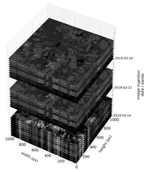
Figure 1. Visualization of how image bands stack in time, as stored in an EOPatch (as the DATA FeatureType).

3.2.7. Cloud and No-Data Masking

To use as many images as possible from the downloaded time range, cloud masking must be implemented. SCL (scene classification layer) is a ready-to-use raster in the Sentinel-2 SAFE folder, and it was used as a preliminary cloud masking solution for the processing pipeline.

The adopted AddMask class abstracts SCL from a zip archive similarly to the case of bands. It resamples the bands to 10 m and clips them by a respective bounding box. SCL is then reclassified to a Boolean array of true (clear) and false (cloudy) pixels in a similar manner to that of the work of Baetens et al. [43]; however, the saturated or defective (pixels) class was counted as valid. SCL also contains a class with no data, representing places where the Sentinel-2 scene has not been captured [42]. Such pixels are also treated as false data. Masks are stored in EOPatches under an arbitrary key as the MASK FeatureType, a four-dimensional NumPy array. There is a single mask for each image (Figure 2 [80]), so the band dimension is always of size one.

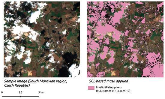
Figure 2. Sample scene classification layer (SCL)-based mask applied on a Sentinel-2 image. Data source: Sentinel-2 image from 14.3.2019.

An additional mechanism was implemented due to accuracy concerns of the Sen2Cor SCL cloud-masking capabilities, as some misclassified clouds in largely cloud-covered images might corrupt classification results. Because the initial download of the images is restricted by the cloud coverage of the whole scene, no attention was paid to the validation of individual EOPatches. The MaskValidation class, inspired by Lubej [17], assesses the SCL mask and returns a Boolean value that indicates whether the invalid (false) pixels have exceeded a user defined threshold. Booleans are forwarded as decision values to the native EOTask SimpleFilterTask, which individually removes undesired images from each EOPatch. Because of this mechanism, the temporal distribution of images may now be unbalanced among EOPatches.

3.2.8. Sentinel-2 Multi-Image Features

Adapting a method devised by Lubej [17], a new class was created for adding multi-image features, such as ratio-images or normalized indices. The Index DataBase is a comprehensive database of formulas for computing some of these multi-image features, including those for Sentinel-2 [81].

The custom EOTask DerivateProduct accepts a user-defined multi-image feature name, bands to be used for the computation and a string formula. It then utilizes key/value pairs in the META_INFO FeatureType (see Section 3.2.6 ) to target the correct band-arrays within an EOPatch.

3.2.9. Data Post-Processing and Sampling For The Classification Stage

Once bands and multi-image features are stored in EOPatches, they need to be prepared for the classification, which is a strong domain of eo-learn. Scikit-learn estimators contain the fit function, which trains the classification model. As a training material, it requires feature vectors of time-independent and band-independent (two-dimensional) pixels, where each such vector belongs to an information class the model should be fit onto [66]. This is a way of continuous reduction of the spectral feature space on the implementation level. The data in EOPatches must first be reformatted before they are reduced in dimensions. The following process, applying for each EOPatch individually, was derived from the approach of Lubej [17,18].

Holding bands and multi-image features apart in EOPatches is ineffective at this point. The native MergeFeatureTask (see also Figure 3) is thus utilized to concatenate all DATA FeatureTypes timewise, along the band dimension. This creates a new four-dimensional array with all potential training data.

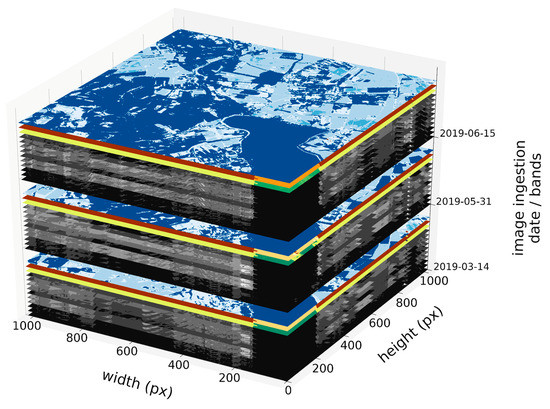
Figure 3. Merged features (three sample multi-image features on the top of bands) stacked in time as the result of the MergeFeatureTask. By this time, they are already filtered by thresholding respective SCL masks (see Section 3.2.7).

The native EOTask LinearInterpolation must then be introduced to interpolate the merged-feature time frames within a selected period and by selected step in days. It first burns respective SCL masks to all image features, converting false pixels to no-data values. New feature time frames are then selected according to the step days, and the closest real feature time frames are interpolated to these points in time. The TIMESTAMP FeatureType of EOPatches is overwritten by new timestamps. This operation presents a great change of the information value because the results are arrays with artificial (interpolated) spectral values. It is nevertheless consistent for all image data in an EOPatch. For instance, if 5 step days are chosen, the resulting temporal series behaves as if each Sentinel-2 5-day-revisit was used (Figure 4).

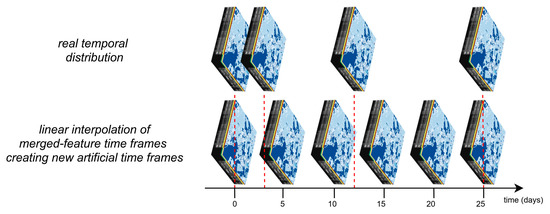
Figure 4. Linear interpolation of merged-feature time frames with five step days chosen.

One reason for interpolation is a potential temporal imbalance of real feature time frames among EOPatches, caused by the additional filtering mechanism (see Section 3.2.7). More importantly, the interpolation is related to the further feature space reduction and feeding such data to a Scikit-learn estimator (see Section 3.2.10). The native PointSamplingTask is used to sample a user-defined number of pixels from interpolated data. This can be imagined as a pan-pixel feature space reduction – the result is a three-dimensional array where each pixel “possesses” temporal stack of features (bands and multi-image features combined).

Finally, the EstimatorParser class reduces the temporal and band dimensions from sampled features and thus returns the required feature vector. It accepts EOPatch IDs to choose only selected patches. All sampled features are merged into a single array, which is then reshaped to a two-dimensional matrix. The rows are the pixels, and the columns are the features stacked temporally. If the interpolation was not introduced, there would be a possibility that for one class and the estimator would train from unequally arranged time frames within several feature vectors. The temporal information would thus corrupt the classification accuracy.

LULC data in the MASK_TIMELESS FeatureType are merged as well. Since they are already a three dimensional array (there is no temporal information), they are reshaped to match the sequence of feature vectors, constituting training class labels. Testing data are obtained similarly, but it is nonetheless meaningful to choose different EOPatches.

3.2.10. Estimator Choice, Model Training, and Prediction

At this point, Sentinel-2 data are prepared for the scikit-learn estimators. It was therefore decided not to implement any wrapper functionalities for interfaces of the scikit-learn library, as they are considered self-contained and have the functionalities for the classification accuracy assessment as well. Moreover, the estimators require different settings for their parameters, which is another complex topic. An example estimator is used in Section 3.3. Some estimators cannot handle no-data values, which can be present in EOPatches. This concerns two cases in particular:

• If multi-image features are included in the classification process, depending on the formula, division by zero can occur. eo-learn handles this problem by substituting a no-data value for the erroneous result.
• If some pixels are masked throughout the whole time series by the SCL mask, they remain unknown and there is nothing to interpolate them from.

The processing pipeline does not solve the problem of no-data values yet; however, the scikit-learn multivariate imputation of missing values [82] can be used to impute the EstimatorParser results. However, to mitigate the decrease in classification quality, the custom NanRemover EOTask was introduced to remove no-data values from sampled pixels of both Sentinel-2 imagery and training data. Once the model is trained, its prediction needs to be adjusted to the format of data in EOPatches. The eo-learn’s PredictPatch repeats a similar process of the EstimatorParser with all data in each EOPatch. The estimator’s predict function is applied to respective feature vectors. These LULC predictions are then reshaped back to a three-dimensional array and stored into EOPatch. Later, they can be exported as GeoTIFF (EOTask ExportToTiff). Accuracy assessment has not been implemented to the pipeline, but it was manually conducted in the example usage experiment.

3.3. Pipeline Demonstration

An area of the South Moravian Region in the Czech Republic was selected to examine the pipeline as a proof-of-concept feasibility demonstration. Open reference cadastral data, besides CLC and UA, at a scale of 1:2000 were obtained from the Registry of Territorial Identification, Addresses, and Real Estates. The cadastral data contain land use information originally in ten classes; however, only eight of them were used. The classes designated Other Surfaces and Hop Field were neither desirable nor applicable within the study area.

The input cadastral map was rasterized with the pixel value of a land-cover information class number and the cell size of 10 m (corresponding to the Sentinel-2 geometric resolution). Because some cadastral parcels were still not in a digital form (thus missing) in the study area, they were handled as no-data in the resulting raster. The 56 Sentinel-2 images were scaled to nine EOPatches, the SCL-based mask was retrieved and scaled alike. The processing operations, described in Section 3.2.6, Section 3.2.7, Section 3.2.8 and Section 3.2.9, were then carried out on the data. The cloud coverage threshold for additional image filtering was set as low as 10% to avoid large areas with no-data values, once the mask is burnt to the merged features at the interpolation. When following Figure 5, the interpolation period was set from 30 March to 16 October 2019, representing a 200-day span. The interpolation step was set to 10 days (virtually two Sentinel- revisits), resulting in 21 interpolated time frames.

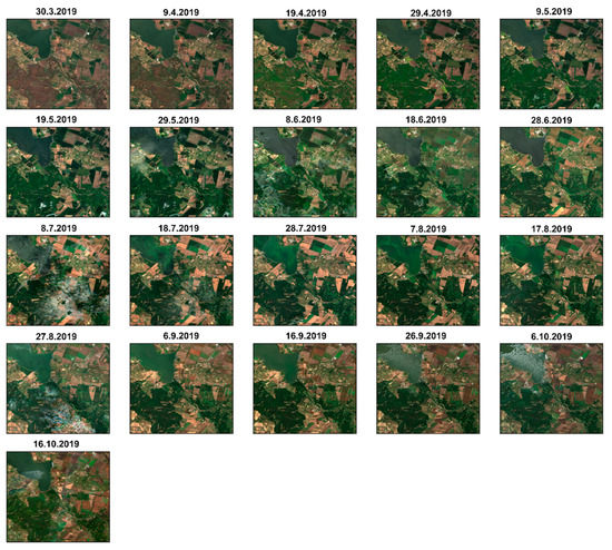
Figure 5. The filtered and interpolated Sentinel-2 time series from 30.3.2019 to 16.10.2019 of feature time frames on the example of EOPatch with ID 7.

In total, 100,000 multi-temporal pixels (feature vectors) were randomly sampled from EOPatches, which were divided in a 5:4 ratio of training patches to test patches. The information class balance in cadaster was chosen as the criterion of selecting EOPatches for the train/test split of the data. Because the number of cadaster information classes was naturally consistent within all EOPatches, Shannon’s entropy (H) was computed for the sampled data [83]. See Table 2, which is an index of diversity among (LULC classes in a single EOPatch) ranging from zero to the logarithm (with any base) of the number of assessed classes, for the results. It was computed as depicted in Equation (1)

$$H={\displaystyle \sum }_{q-1}^q\ast p_i\ast \log p_i$$

(1)

where q is number of information classes, i is a class, and p is a ratio of class frequency and the sum of class values of pixels sampled within an EOPatch.

Table 2. Shannon’s entropy as an inter-class balance criterion for each EOPatch used to select training and test sets from the sampled data. Note: H stands for Shannon’s entropy, which is a dimensionless number.

EOPatch ID	H	H Rank	Selected for
0	1.110	8	Testing
1	0.895	9	Training
2	1.281	7	Training
3	1.476	4	Testing
4	1.575	3	Training
5	1.424	5	Training
6	1.584	2	Testing
7	1.679	1	Training
8	1.287	6	Testing

In the conducted proof-of-concept, the range of values of H was from 0 to log(8), as there were eight information classes in this experiment. From a high H value, it can be assumed the classes were diverse and thus balanced in an EOPatch. The EOPatches for training and testing were chosen alternately with decreasing H, starting with the choice for training. At the end, there were 500,000 unique samples for both training and testing.

The feature space of sampled features was then reduced to feature vectors and assigned with the respective LULC information class number for both training and test sets.

The LightGBM estimator [47] was selected for the classification to become at least partly available to compare the results with the example in the work of Lubej [17,18] and eo-learn [48,49]. The LightGBM estimator is an effective algorithm based on the machine learning method of gradient boosting decision tree (GBDT) that should be used for larger training datasets (which the cadaster data certainly were). Discussing and setting up various parameters for the best classification results have been left for future research; therefore, the same parameters as in [17,49] were used.

An analysis should have been made prior to setting the LightGBM estimator. However, more than a hundred set up parameters were identified. The amount of required work would have considerably exceeded the possibilities of this limited feasibility study. Setting up all the required parameters accordingly remains a possibility in terms of future work. The labelled feature vectors were trained and predicted, the prediction was tested on the generated test data from the remaining patches, and the best result was chosen. The confusion matrix, a commonly used classification accuracy assessment tool [84], was obtained to review the results.

4. Results

4.1. Processing Pipeline, Experimental Outputs and Integration to OLU/OLC

The processing pipeline for LULC classification using Sentinel-2 imagery is divided into two custom Python modules (see Supplementary Materials) and a Jupyter Notebook with the implementation applied to the example usage experiment (also in the Supplementary Materials). Each file is described with explanatory comments, and the classes and their methods contain docstrings to understand their meaning.

4.2. Experimental Outputs

The usage experiment showed a good OA of 85.9% and yielded a classified LULC map of the study area in the southern part of the South Moravian Region (Appendix A).

The confusion matrix in Table 3 suggests that there were both very well and very poorly predicted LULC classes (considering provider accuracy, i.e., the ratio between well predicted pixels and testing pixels). The most accurately predicted were forests (91.5%), arable land (87.9%), and water (87.2%). On the other hand, the classification performed very poorly on permanent grasslands (45.2%), which are very diverse surfaces. They were most often misclassified as arable land and forests. A similarly low accuracy was seen in the prediction of gardens, which also appear in various forms. Built-up areas were predicted fairly well (accuracy of 75%); they were most often misclassified as arable land, having similar spectral behavior after harvest, and gardens, which are in close proximity. Surprising results were achieved in predicting vineyards, with an accuracy of 67.5%, which can be attributed to common spectral behavior of most vineyard samples. A more detailed explanation on the classification process is provided in the discussion section.

Table 3. Confusion matrix of the LULC (land use/land cover) classification experiment in the southern part of the South Moravian region. The achieved overall accuracy (OA) was 85.9%.

P	Arable Land	Vine-Yard	Garden	Orchard	Permanent Grassland	Forest	Water	Built-Up Areas	Sum of Pixels
Arable land	312,481	4853	1522	725	1170	1865	1236	1705	325,557
Vineyard	10,235	15,518	162	306	110	286	102	95	26,814
Garden	5727	581	2387	328	217	298	22	1459	11,019
Orchard	5427	902	79	3485	500	268	27	48	10,736
Permanent grassland	7892	355	90	77	2436	1642	469	120	13,081
Forest	6824	409	206	66	671	60,947	967	226	70,316
Water	3084	39	139	483	177	1140	20,328	278	25,668
Built-up areas and roads	3644	319	562	40	111	189	165	11,779	16,809
Sum of pixels	355,314	22,976	5147	5510	5392	66,635	23,316	15,710	500,000
Omission error	12.1%	31.1%	42.7%	36.8%	54.8%	8.5%	12.8%	25.0%
Commission error	4.0%	42.1%	78.3%	67.5%	81.4%	13.3%	20.8%	29.9%
Provider accuracy	87.9%	67.5%	46.4%	63.2%	45.2%	91.5%	87.2%	75.0%

In Figure 6, the prediction and the original cadaster training data can be compared. The prediction favored built-up areas and forests and extended them slightly over the surrounding classes. Some paths and roads were interrupted as the 10 m resolution was not sufficient to facilitate identification of continuous pixels of linear features. The prediction was also affected by a common salt-and-pepper effect, which is a data noise caused by individual pixels being misclassified within a large body of a different class. This can be resolved by various noise removal techniques [84]; however, this was not conducted in this experiment in order to compare the raw data. Some places (shown in grey) in the original cadastral data did not contain land cover information. Considering that Sentinel-2 data cover the whole study area, such places were naturally predicted. It can thus be concluded that even within the comprehensive Czech cadastral data, some new information was supplied.

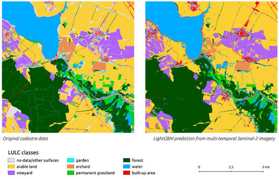
Figure 6. Comparison of original cadaster data and the LightGBM prediction. Sources: Sentinel-2 imagery from 30.3 to 16.10 [80], Czech cadastral map [85].

A single-map comparison is provided in Figure 7, where the original cadaster data and the LightGBM prediction were erased and the result was reclassified to a binary raster of class change/no change. If substitution of original no-data with new values is not considered, the most misclassified LULC class was that of permanent grasslands, which corresponded to the overall results of the classification. Class mismatch was found to increase in more fragmented places, especially in the built-up areas, which are often spatially intertwined with poorly classified gardens.

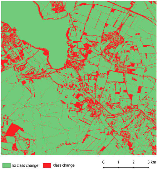
Figure 7. Monitoring class mismatch between the original cadaster data and the LightGBM prediction to visually assess the results of the classification. Sources: Sentinel-2 imagery from 30.3 to 16.10.2019 [80], Czech cadastral map [85].

4.3. Integration of Pipeline to OLU/OLC

The integration of the processing pipeline and its results to OLU/OLC has to be put in a context with the new OLU/OLC data models (not publicly available as of December 2020). The model is designed to handle contributing data apart from the processed data to ensure smooth update and to avoid compatibility issues. The results from the processing pipelines are primarily in a raster format (GeoTiff in the usage experiment). It is suggested that once that LULC dataset is predicted over an area, EOPatches could be utilized as the basis for map tiles. Stored outside of the processed OLU/OLC map, they can still be updated by repeated predictions. Nonetheless, the tiles have to be vectorized and forwarded to the OLU/OLC compilation process (as an LULC layer). If classification post-processing is thoroughly examined, the vectorized geometries can constitute OLU/OLC objects. The integration of the developed proof-of-concept pipeline to OLU/OLC is being prepared as a follow-up paper, with emphasis on data modelling aspects.

5. Discussion

Table 4 provides an overview on the results presented in this paper alongside comparison with related work.

Table 4. Summary of the discussion points to the main goals of the presented paper (1–4) with respect to related work.

Discussion Points To Defined Goals	Related Work
(1) Collects Sentinel-2 Imagery   A collection of Sentinel-2 imagery is publicly available at Sentinel Hub (https://www.sentinel-hub.com/). This paper presents an open and free-of-charge solution contrasting with the paid Sentinel Hub. Moreover, the presented research is modular. The Sentinel-2 imagery collection module (see Supplementary Materials) can be deployed to any open Sentinel-2 based solution.   The following features needed to be newly developed or re-created: (a) Semi-automatic satellite data download. (b) Batch input of Sentinel-2 imagery and raw file handling. (c) Image preprocessing: selection of desired bands and resampling to 20 m (or arbitrary) resolution. (d) Cloud masking using SCL. (e) Setting up a workflow for regular updates of a specific dataset.	The methodology of Lubej [17,18] avoided the functionality of the developed module by direct connection to the (paid) Web Coverage Service (WCS) interface of the Sentinel Hub.   Similar parts (from the paid Sentinel Hub) were also used by Lubej [17,18], especially in the preparation of ground data (rasterization, sampling to patches, and selecting train/test samples), imagery interpolation, and sampling.
(2) Filters Cloudiness through Multitemporal Vectors   In this case, too, a paid module named ‘Sen2Cloudless’ is provided as a functionality of the Sentinel Hub. The presented approach offers a newly developed open and free-of-charge alternative.	In contrast to the work of Lubej [17,18], masking was newly developed with the functionality equivalent to the subscription-based features of the Sentinel Hub platform. The used cloudiness filtering originated from the Sen2Cor product [42].   A more advanced cloudiness filtering is available under the designation ‘Fmask’ [38]. Nevertheless, this filter has not been implemented in the Python language at the time when this study was being prepared due to certain issues in ‘Fmask’ implementation.
(3) Examines the Possibility of the Pipeline to Perform LULC Classification over the Imagery   Throughout the study, the main emphasis was to populate the data gaps within the open land use/open land cover (OLU/OLC) datasets. Such gaps appeared commonly, typically due to missing information in input data: cadastral maps, Urban Atlas (UA), and Corinne Land Cover (CLC).   A feasibility study on classification performance over the imagery was conducted on an area larger than 7000 km2.   The presented OA (85.9%) arose as a consequence of the high percentage (71.1%) of arable land class in the conducted experiment. It seems that the ‘learning effect’ favored the most represented class, arable land.   The lowest OA values were achieved in gardens (46.4%) and permanent grasslands (45.2%). Gardens were a priori expected to become the class with the worst results due to its heterogeneity. Some pixels containing gardens were mainly misclassified as arable land (in a half of the cases) and less commonly as built-up areas, vineyards, orchards, and forests. Permanent grasslands were mainly misclassified as arable land (in about 60% of the cases). This result seemed to originate from the time span of the satellite images series.   Verifications were performed on pseudo-continuous (vector) ‘ground truth’ data, represented by the cadastral maps at a scale of 1:2000, reclassified to spatial resolution equal to 10 m.   Accuracy assessment followed the methodology of ‘random stratified sampling design.’ Shannon’s entropy helped to expose hidden errors that could be caused by favoring underrepresented classes. Using Shannon’s entropy was a novel approach in comparison to the state-of-the-art.   In the future, the accuracy of heterogeneous classes, such as gardens and orchards, could be assessed using a cluster sampling design to mitigate outsourcing their pixels to different classes. The grey level co-occurrence matrix (GLCM) should be used to improve the classification matrix (see Section 5.1 for details).	Schultz et al. [86] populated an LULC dataset through another approach. They attempted to fill in the gaps by remote sensing (RS) of classified land cover data from OpenStreetMap tags. However, the achieved results do not seem convincing [86].   The related research takes discrete information from field measurements, which usually comprise tens or hundreds of discrete points, into account [87]. Using a large test sample could lead to an over-powered testing, as suggested by Foody [87].   The accuracy assessment methodology of ‘random stratified sampling design’ was recommended in [88,89]. Foody [87] noted that using Shannon’s entropy exposes the false negatives.
(4) Semi-Automatically Updates OLU/OLC Databases Accordingly   The presented approach was found to be feasible. The full potential of the developed pipeline appears when combining the pipeline with the open data model of the OLU/OLC datasets (currently being prepared as a follow-up paper).   The discussion regarding this point is provided in Section 5.1 due to its complexity and extent.	The need for semi-automatic updates of LULC is emphasized in similar research, as presented by Weigand et al. [27], with an OA of 80–93.1%, and Malinowski et al. [90], with an OA of 89%. Both were considerably larger studies, thus proving that such a workflow can have a large-scale LU/LC derivation potential.

Selected points are described in more detail in Section 5.1 and Section 5.2 as an extension of Table 4.

5.1. Processing Pipeline Prospects and Its Significance for OLU/OLC

The processing pipeline is an open proof-of-concept solution for refining OLU/OLC. Its principle lies in processing Sentinel-2 imagery for spectral-based supervised classification while the training data can be selected freely. The pipeline prepares the data for scikit-learn machine learning estimators. Some design aspects were adapted from the LULC mapping methodology of the eo-learn library’s developers [17,49], who performed the land cover classification of Slovenia on the basis of the Slovenian Land Parcel Identification System (LPIS) and achieved a good OA of 91.2%. The proposed processing pipeline was inspired by their approach; nevertheless, it came up with custom solutions (see Table 4 for details).

The main contributing resources of OLU/OLC at the time of writing this paper were CLC and UA. These datasets were guaranteed within the whole spatial extent of OLU/OLC, i.e., in areas where finer LULC information is unavailable or it is entirely missing. The processing pipeline laid grounds to relieve OLU/OLC from dependency on these datasets. It particularly attempted to increase the spatial resolution, diminish the dataset creation periodicity, and provide LULC information in regions where CLC and UA data are absent.

It is to be noted that the processing pipeline has not yet achieved the ability to classify land use in the true sense of word. Land use information is often retrieved using image classification techniques that accommodate contextual information, particularly object-based methods [5,90]. These should be further examined with regard to the processing pipeline, preferably in synergy with spectral information for the best performance [45]. Ma et al. [3] nonetheless concluded that object-based methods have been practiced over small territories (with a mean area of only 300 ha), and their application over larger areas is a subject for future research. Many studies dealing with land use information retrieval also follow commercial, very fine resolution imagery that cannot be freely utilized in OLU/OLC. It is clear that the pixel-wise approach along with the 10–20 m resolution of Sentinel-2 imagery, used in the pipeline, is too coarse for retrieving subtle semantic variations of land uses (like the approach of Palma [8]). Adopting advanced techniques is a proposed future improvement of the pipeline.

One of the biggest advantages of the pipeline is that it can naturally handle multi-temporal imagery. Temporal information is a carrier structure for the feature vectors as utilized in this paper. The validation of multi-temporal classification can also be problematic as training or test data (ground truth data) remain static while the real earth-features can change through time.

To preserve the 10 m geometric resolution of the final classification result, only 10 and 20 m Sentinel-2 bands were used in the pipeline. This corresponded with the approach of Lubej [18], who achieved high overall classification accuracies even with fewer bands used in the process. The decision to upscale 20 m bands to a 10 m resolution was made, although it reduced spectral information reliability to some extent. Zheng et al. [4] similarly used nearest neighbor interpolation to assess the effects of upscaling and downscaling of Sentinel-2 data and proved that classification accuracies diminished when upscaling 10 and 20 m bands. Surprisingly, the straightforward nearest neighbor downscaling was the most beneficial for LULC classification purposes. For future development of the pipeline, downscaling should thus be exercised for better classification accuracies because the geometric resolution of 20 × 20 m still outperforms the MMU of CLC in general and the MMU of UA in rural areas.

Thanks to the Sentinelsat API [72], the pipeline has a continuous access to the Copernicus Open Access Hub [73] and, thus, to the full time series of Sentinel imagery. Their automated processing outsources several tasks, such as downloading and unzipping images, file format handling, image resampling, subsetting, and masking from the operator, who can then devote more time to the classification process itself.

The character of the pipeline allows for LULC prediction over a vast area of interest while avoiding high computational demands thanks to the concept of EOPatches. This is a key to the rapid extension of OLU/OLC LULC information to areas out of the extent of CLC or UA. For mass LULC classification, it is critical for the pipeline to be able to automatically mosaic and reproject imagery in the future. The incorporation of multi-image features in the pipeline is still a basic solution, so not all such features can be obtained (e.g., pan-sharpening or image principal component analysis). On the other hand, even simple vegetation and other spectral indices have been reliably used for change detection (i.e., [24]), which is another potential development direction for OLU/OLC, emphasized especially by the umbrella organization Plan4All. In its current version, eo-learn further contains EOTasks for grey level co-occurrence matrix (GLCM) computation and the extraction of various textural variables, which could be further added among training features in the pipeline. According to the review of Khatami, Mountrakis, and Stehman [9] (2016), textural information has been the most effective accuracy-improving feature for spectral-based classification (improving OA by 12.1% on average).

5.2. Conducted Experiment Discussion

The example usage experiment should have primarily demonstrated the usage of the processing pipeline without primary attention paid to the classification parameters setup. The LightGBM estimator, using the 200-day time series of Sentinel-2 images and the LULC information from the Czech cadaster, offered an OA of 85.9%. Some LULC classes, such as permanent grasslands and gardens, were nonetheless poorly classified. A comparison should be made with the work of Lubej [17,18] and eo-learn [48,49], from which the pipeline adapted some of its design aspects. In their eo-learn showcase example, they classified land cover on the basis of the Slovenian LPIS. They had three more classes (snow, tundra, and shrubland), but the classification was otherwise similar to that in the experiment presented in this paper. With an equally set up estimator, they achieved a much better OA (91.2%). They nonetheless had access to the pre-processed data of the Sentinel Hub platform with machine learning-based cloud masking algorithm and had the “developer knowledge” of the eo-learn library.

The proposed pipeline usage faced several challenges when being deployed to OLU/OLC. Eight information classes are not sufficient to populate the fine HILUCS classification accordingly. The number and identification of information classes stems from the used underlying datasets, primarily the structure of the Czech cadaster. To use the pipeline in other regions, the model will have to be re-trained on a more typical landscape of those regions, and a custom training dataset will probably have to be used. As suggested by Nguyen et al. [30], the extension of merged-feature time frames for cloud-filtering could be required for tropical regions due to the complexity of biophysical environment (clouds and haze). In terms of future research, it is nonetheless interesting to examine how LULC predictions will behave if trained by other international, national, or regional datasets. This can help assess the trade-off for putting less effort into training data collection.

6. Conclusions

The main result of the research described in this paper is an open proof-of-concept machine learning-based processing pipeline for automatic Sentinel-2 imagery collection, cloudiness filtering, LULC classifications, and updates of OLU/OLC. The pipeline was developed in the Python environment, especially using the eo-learn library and some other Python libraries. It can process multitemporal Sentinel-2 imagery to a form that can be forwarded to various scikit-learn estimators.

In comparison with the current OLU/OLC background datasets, its latest design, as followed within the conducted experiment, provides more spatially precise results that can be retrieved in near real time. That opens a possibility for OLU/OLC to amend its own LULC data and reduce dependence on primarily assumed input datasets (e.g., CORINE Land Cover, and Urban Atlas). Though experimentally tested with a fair result (OA of 85.9%), the classification results are not yet ideal, and more research needs to be done to provide reliable land-use-like data with a higher accuracy and a number of information classes. During the process, the software engineering tasks turned out to be a significant means of understanding OLU/OLC as a system and choosing the design decisions for the processing pipeline.

Despite the progress achieved in the conducted experiments, more work is needed to amend intrinsic OLU/OLC LULC information, especially by improving the classification process itself. Similarly, the possibilities of verifying LULC information in OLU/OLC must be further investigated. Special attention should also be paid to clarifying the licensing model of OLU/OLC and to analyzing the negative implications of fusing various LULC and other, often semantically different, data.

References

- Fisher, P.F.; Comber, A.; Wadsworth, R. Land use and land cover: Contradiction or complement. In Re-presenting GIS; John Wiley: Chichester, NH, USA, 2005; pp. 85–98. [Google Scholar]
- Castelluccio, M.; Poggi, G.; Sansone, C.; Verdoliva, L. Land Use Classification in Remote Sensing Images by Convolutional Neural Networks. ArXiv Comput. Sci. 2015, 1–11. Available online: https://arxiv.org/abs/1508.00092 (accessed on 2 December 2020).
- Ma, L.; Li, M.; Ma, X.; Cheng, L.; Du, P.; Liu, Y. A review of supervised object-based land-cover image classification. ISPRS J. Photogramm. Remote Sens. 2017, 130, 277–293. [Google Scholar] [CrossRef]
- Zheng, H.; Du, P.; Chen, J.; Xia, J.; Li, E.; Xu, Z.; Li, X.; Yokoya, N. Performance Evaluation of Downscaling Sentinel-2 Imagery for Land Use and Land Cover Classification by Spectral-Spatial Features. Remote Sens. 2017, 9, 1274. [Google Scholar] [CrossRef]
- Rosina, K.; Batista e Silva, F.; Vizcaino, P.; Marín Herrera, M.; Freire, S.; Schiavina, M. Increasing the detail of European land use/cover data by combining heterogeneous data sets. Int. J. Digit. Earth 2020, 13, 602–626. [Google Scholar] [CrossRef]
- Čerba, O. Ontologie Jako Nástroj pro Návrhy Datových Modelů Vybraných Témat Příloh Směrnice INSPIRE. Ph.D. Thesis, Charles University, Prague, Czech Republic, 2012. Available online: http://hdl.handle.net/20.500.11956/47841 (accessed on 2 December 2020).
- Feiden, K.; Kruse, F.; Řezník, T.; Kubíček, P.; Schentz, H.; Eberhardt, E.; Baritz, R. Best Practice Network GS SOIL Promoting Access to European, Interoperable and INSPIRE Compliant Soil Information. In Environmental Software Systems. Frameworks of eEnvironment; IFIP Advances in Information and Communication Technology; Springer: Berlin/Heidelberg, Germany, 2011; pp. 226–234. ISBN 978-3-642-22284-9. [Google Scholar] [CrossRef]
- Palma, R.; Reznik, T.; Esbrí, M.; Charvat, K.; Mazurek, C. An INSPIRE-Based Vocabulary for the Publication of Agricultural Linked Data. In Ontology Engineering; Lecture Notes in Computer Science; Springer International Publishing: Cham, Switzerland, 2016; pp. 124–133. ISBN 978-3-319-33244-4. Available online: http://doi-org-443.webvpn.fjmu.edu.cn/10.1007/978-3-319-33245-1_13 (accessed on 2 December 2020).
- Khatami, R.; Mountrakis, G.; Stehman, S.V. A meta-analysis of remote sensing research on supervised pixel-based land-cover image classification processes: General guidelines for practitioners and future research. Remote Sens. Environ. 2016, 177, 89–100. [Google Scholar] [CrossRef]
- INSPIRE Data Specification on Land Cover—Technical Guidelines. Available online: https://inspire.ec.europa.eu/id/document/tg/lc (accessed on 2 December 2020).
- European Environment Agency. CORINE Land Cover. Available online: https://land.copernicus.eu/pan-european/corine-land-cover (accessed on 2 December 2020).
- Copernicus Programme. Urban Atlas. Available online: https://land.copernicus.eu/local/urban-atlas (accessed on 2 December 2020).
- INSPIRE Land Cover and Land Use Data Specifications. Available online: https://eurogeographics.org/wp-content/uploads/2018/04/2.-INSPIRE-Specification_Lena_0.pdf (accessed on 2 December 2020).
- OSM. Landuse Landcover. Available online: https://osmlanduse.org/#12/8.7/49.4/0/ (accessed on 2 December 2020).
- USGS. Land Cover Data Overview. Available online: https://www.usgs.gov/core-science-systems/science-analytics-and-synthesis/gap/science/land-cover-data-overview?qt-science_center_objects=0#qt-science_center_objects (accessed on 2 December 2020).
- FAO. Global Land Cover SHARE (GLC-SHARE). Available online: http://www.fao.org/uploads/media/glc-share-doc.pdf (accessed on 2 December 2020).
- Lubej, M. Land Cover Classification with Eo-Learn: Part 1, Medium. Available online: https://medium.com/sentinel-hub/land-cover-classification-with-eo-learn-part-1-2471e8098195 (accessed on 2 December 2020).
- Lubej, M. Land Cover Classification with Eo-Learn: Part 2, Medium. Available online: https://medium.com/sentinel-hub/land-cover-classification-with-eo-learn-part-2-bd9aa86f8500 (accessed on 2 December 2020).
- Sibanda, M.; Mutanga, O.; Rouget, M. Examining the potential of Sentinel-2 MSI spectral resolution in quantifying above ground biomass across different fertilizer treatments. ISPRS J. Photogramm. Remote Sens. 2015, 110, 55–65. [Google Scholar] [CrossRef]
- Pesaresi, M.; Corbane, C.; Julea, A.; Florczyk, A.; Syrris, V.; Soille, P. Assessment of the Added-Value of Sentinel-2 for Detecting Built-up Areas. Remote Sens. 2016, 8, 299. [Google Scholar] [CrossRef]
- Korhonen, L.; Hadi; Packalen, P.; Rautiainen, M. Comparison of Sentinel-2 and Landsat 8 in the estimation of boreal forest canopy cover and leaf area index. Remote Sens. Environ. 2017, 195, 259–274. [Google Scholar] [CrossRef]
- Vuolo, F.; Neuwirth, M.; Immitzer, M.; Atzberger, C.; Ng, W.-T. How much does multi-temporal Sentinel-2 data improve crop type classification? Int. J. Appl. Earth Obs. Geoinf. 2018, 72, 122–130. [Google Scholar] [CrossRef]
- Caballero, I.; Ruiz, J.; Navarro, G. Sentinel-2 Satellites Provide Near-Real Time Evaluation of Catastrophic Floods in the West Mediterranean. Water 2019, 11, 2499. [Google Scholar] [CrossRef]
- Kuc, G.; Chormański, J. Sentinel-2 Imagery for Mapping and Monitoring Imperviousness in Urban Areas. ISPRS Int. Arch. Photogramm. Remote Sens. Spat. Inf. Sci. 2019, XLII-1/W2, 43–47. [Google Scholar] [CrossRef]
- Řezník, T.; Pavelka, T.; Herman, L.; Lukas, V.; Širůček, P.; Leitgeb, Š.; Leitner, F. Prediction of Yield Productivity Zones from Landsat 8 and Sentinel-2A/B and Their Evaluation Using Farm Machinery Measurements. Remote Sens. 2020, 12, 1917. [Google Scholar] [CrossRef]
- Bruzzone, L.; Bovolo, F.; Paris, C.; Solano-Correa, Y.T.; Zanetti, M.; Fernandez-Prieto, D. Analysis of multitemporal Sentinel-2 images in the framework of the ESA Scientific Exploitation of Operational Missions. In Proceedings of the 2017 9th International Workshop on the Analysis of Multitemporal Remote Sensing Images (MultiTemp), Brugge, Belgium, 27–29 June 2017; IEEE: New York, NY, USA, 2017; pp. 1–4. [Google Scholar] [CrossRef]
- Phiri, D.; Simwanda, M.; Salekin, S.; Nyirenda, V.R.; Murayama, Y.; Ranagalage, M. Sentinel-2 Data for Land Cover/Use Mapping: A Review. Remote Sens. 2020, 12, 2291. [Google Scholar] [CrossRef]
- Cavur, M.; Duzgun, H.S.; Kemec, S.; Demirkan, D.C. Land use and land cover classification of sentinel 2-a: St Petersburg case study. ISPRS Int. Arch. Photogramm. Remote Sens. Spat. Inf. Sci. 2019, XLII-1/W2, 13–16. [Google Scholar] [CrossRef]
- Weigand, M.; Staab, J.; Wurm, M.; Taubenböck, H. Spatial and semantic effects of LUCAS samples on fully automated land use/land cover classification in high-resolution Sentinel-2 data. Int. J. Appl. Earth Obs. Geoinf. 2020, 88. [Google Scholar] [CrossRef]
- Nguyen, H.T.T.; Doan, T.M.; Tomppo, E.; McRoberts, R.E. Land Use/Land Cover Mapping Using Multitemporal Sentinel-2 Imagery and Four Classification Methods—A Case Study from Dak Nong, Vietnam. Remote Sens. 2020, 12, 1367. [Google Scholar] [CrossRef]
- Ienco, D.; Interdonato, R.; Gaetano, R.; Ho Tong Minh, D. Combining Sentinel-1 and Sentinel-2 Satellite Image Time Series for land cover mapping via a multi-source deep learning architecture. ISPRS J. Photogramm. Remote Sens. 2019, 158, 11–22. [Google Scholar] [CrossRef]
- Rumora, L.; Miler, M.; Medak, D. Impact of Various Atmospheric Corrections on Sentinel-2 Land Cover Classification Accuracy Using Machine Learning Classifiers. ISPRS Int. J. Geo-Inf. 2020, 9, 277. [Google Scholar] [CrossRef]
- Jain, M.; Dawa, D.; Mehta, R.; Dimri, A.P.; Pandit, M.K. Monitoring land use change and its drivers in Delhi, India using multi-temporal satellite data. Modeling Earth Syst. Environ. 2016, 2. [Google Scholar] [CrossRef]
- Talukdar, S.; Singha, P.; Mahato, S.; Shahfahad; Pal, S.; Liou, Y.-A.; Rahman, A. Land-Use Land-Cover Classification by Machine Learning Classifiers for Satellite Observations—A Review. Remote Sens. 2020, 12, 1135. [Google Scholar] [CrossRef]
- Liu, C.-C.; Zhang, Y.-C.; Chen, P.-Y.; Lai, C.-C.; Chen, Y.-H.; Cheng, J.-H.; Ko, M.-H. Clouds Classification from Sentinel-2 Imagery with Deep Residual Learning and Semantic Image Segmentation. Remote Sens. 2019, 11, 119. [Google Scholar] [CrossRef]
- Hagolle, O.; Huc, M.; Villa Pascual, D.; Dedieu, G. A Multi-Temporal and Multi-Spectral Method to Estimate Aerosol Optical Thickness over Land, for the Atmospheric Correction of FormoSat-2, LandSat, VENμS and Sentinel-2 Images. Remote Sens. 2015, 7, 2668–2691. [Google Scholar] [CrossRef]
- Hollstein, A.; Segl, K.; Guanter, L.; Brell, M.; Enesco, M. Ready-to-Use Methods for the Detection of Clouds, Cirrus, Snow, Shadow, Water and Clear Sky Pixels in Sentinel-2 MSI Images. Remote Sens. 2016, 8, 666. [Google Scholar] [CrossRef]
- Zhu, Z.; Woodcock, C.E. Object-based cloud and cloud shadow detection in Landsat imagery. Remote Sens. Environ. 2012, 118, 83–94. [Google Scholar] [CrossRef]
- Qiu, S.; Zhu, Z.; He, B. Fmask 4.0: Improved cloud and cloud shadow detection in Landsats 4–8 and Sentinel-2 imagery. Remote Sens. Environ. 2019, 231. [Google Scholar] [CrossRef]
- Zhu, Z.; Wang, S.; Woodcock, C.E. Improvement and expansion of the Fmask algorithm: Cloud, cloud shadow, and snow detection for Landsats 4–7, 8, and Sentinel 2 images. Remote Sens. Environ. 2015, 159, 269–277. [Google Scholar] [CrossRef]
- Flood, N.; Gillingham, S. PythonFmask Documentation, Release 0.5.4. Available online: http://www.pythonfmask.org/en/latest/#python-developer-documentation (accessed on 2 December 2020).
- Main-Knorn, M.; Pflug, B.; Louis, J.; Debaecker, V.; Müller-Wilm, U.; Gascon, F.; Bruzzone, L.; Bovolo, F.; Benediktsson, J.A. Sen2Cor for Sentinel-2. In Proceedings of the Image and Signal Processing for Remote Sensing XXIII, Warsaw, Poland, 11–13 September 2017; SPIE: Washington, DC, USA, 2017; p. 3. [Google Scholar] [CrossRef]
- Baetens, L.; Desjardins, C.; Hagolle, O. Validation of Copernicus Sentinel-2 Cloud Masks Obtained from MAJA, Sen2Cor, and FMask Processors Using Reference Cloud Masks Generated with a Supervised Active Learning Procedure. Remote Sens. 2019, 11, 433. [Google Scholar] [CrossRef]
- Centre National d’Études Spatiales. MAJA. Available online: https://logiciels.cnes.fr/en/content/MAJA (accessed on 2 December 2020).
- Zhao, B.; Zhong, Y.; Zhang, L. A spectral–structural bag-of-features scene classifier for very high spatial resolution remote sensing imagery. ISPRS J. Photogramm. Remote Sens. 2016, 116, 73–85. [Google Scholar] [CrossRef]
- Abdi, A.M. Land cover and land use classification performance of machine learning algorithms in a boreal landscape using Sentinel-2 data. GIScience Remote Sens. 2020, 57, 1–20. [Google Scholar] [CrossRef]
- Ke, G.; Meng, Q.; Finley, T.; Wang, T.; Chen, W.; Ma, W.; Ye, Q.; Liu, T.-Y. LightGBM: A Highly Efficient Gradient Boosting Decision Tree. In Advances in Neural Information Processing Systems; Guyon, I., Luxburg, U.V., Bengio, S., Wallach, H., Fergus, R., Vishwanathan, S., Garnett, R., Eds.; 2017; pp. 3146–3154. Available online: https://arxiv.org/pdf/1810.10380.pdf (accessed on 2 December 2020).
- EO-LEARN. 0.4.1 Documentation. Available online: https://eo-learn.readthedocs.io/en/latest/index.html# (accessed on 2 December 2020).
- EO-LEARN. 0.7.4 Documentation. Available online: https://eo-learn.readthedocs.io/en/latest/index.html (accessed on 2 December 2020).
- OLU. Open Land Use. Available online: https://sdi4apps.eu/open_land_use/ (accessed on 2 December 2020).
- Mildorf, T. Uptake of Open Geographic Information through Innovative Services Based on Linked Data; Final Report; University of West Bohemia: Pilsen, Czech Republic, 2017; 30p, Available online: https://sdi4apps.eu/wp-content/uploads/2017/06/final_report_07.pdf (accessed on 2 December 2020).
- Kožuch, D.; Charvát, K.; Mildorf, T. Open Land Use Map. Available online: https://eurogeographics.org/wp-content/uploads/2018/04/5.Open_Land_Use_bruxelles.pdf (accessed on 2 December 2020).
- Kožuch, D.; Čerba, O.; Charvát, K.; Bērziņš, R.; Charvát, K., Jr. Open Land-Use Map. 2015. Available online: https://sdi4apps.eu/open_land_use/ (accessed on 2 December 2020).
- OGC. OpenGIS Web Map Server Implementation Specification; Open Geospatial Consortium: Wayland, MA, USA; 85p, Available online: https://www.ogc.org/standards/wms (accessed on 2 December 2020).
- OGC. OpenGIS Web Feature Service 2.0 Interface Standard; Open Geospatial Consortium: Wayland, MA, USA; 253p, Available online: https://www.ogc.org/standards/wfs (accessed on 2 December 2020).
- Dijkstra, L.; Poelman, H.; Veneri, P. The EU-OECD definition of a functional urban area. In OECD Regional Development Working Papers 2019; OECD Publishing: Paris, French, 2019; pp. 1–19. ISSN 20737009. [Google Scholar] [CrossRef]
- European Commission. Copernicus—Europe’s Eyes on Earth; European Commission: Brussels, Belgium; Available online: https://www.copernicus.eu/en (accessed on 2 December 2020).
- Kosztra, B.; Büttner, G.; Soukup, T.; Sousa, A.; Langanke, T. CLC2018 Technical Guidelines. European Enivonment Agency 2017; Environment Agency: Wien, Austria, 2017; 61p, Available online: https://land.copernicus.eu/user-corner/technical-library/clc2018technicalguidelines_final.pdf (accessed on 2 December 2020).
- RÚIAN. Registry of Territorial Identification, Addresses and Real Estates. Available online: https://geoportal.cuzk.cz/mGeoportal/?c=dSady_RUIAN_A.EN&f=paticka.EN&lng=EN (accessed on 2 December 2020).
- European Space Agency. User Guides—Sentinel-2. Available online: https://sentinel.esa.int/web/sentinel/user-guides/sentinel-2-msi (accessed on 2 December 2020).
- European Space Agency. Sentinel-2 User Handbook; ESA: Paris, French; 64p, Available online: https://sentinels.copernicus.eu/documents/247904/685211/Sentinel-2_User_Handbook (accessed on 2 December 2020).
- U.S. Geological Survey. USGS EROS Archive—Sentinel-2—Comparison of Sentinel-2 and Landsat. Available online: https://www.usgs.gov/centers/eros/science/usgs-eros-archive-sentinel-2-comparison-sentinel2-and-landsat?qt-science_center_objects=0#qt-science_center_objects (accessed on 2 December 2020).
- Kussul, N.; Lavreniuk, M.; Skakun, S.; Shelestov, A. Deep Learning Classification of Land Cover and Crop Types Using Remote Sensing Data. IEEE Geosci. Remote Sens. Lett. 2017, 14, 778–782. [Google Scholar] [CrossRef]
- Verburg, P.H.; Neumann, K.; Nol, L. Challenges in using land use and land cover data for global change studies. Glob. Chang. Biol. 2011, 17, 974–989. [Google Scholar] [CrossRef]
- Pedregosa, F.; Varoquaux, G.; Gramfort, A.; Michel, V.; Thirion, B.; Grisel, O.; Blondel, M.; Prettenhofer, P.; Weiss, R.; Dubourg, V.; et al. Scikit-Learn: Machine Learning in Python. J. Mach. Learn. Res. 2011, 12, 2826–2830. Available online: http://jmlr.org/papers/v12/pedregosa11a.html (accessed on 2 December 2020).
- SCIKIT-LEARN DEVELOPERS. An Introduction to Machine Learning with Scikitlearn—Scikit-Learn 0.23.1 Documentation. Available online: https://scikit-learn.org/stable/tutorial/basic/tutorial.html (accessed on 2 December 2020).
- SINERGISE. Sentinel Hub 3.0.2 Documentation. Available online: https://sentinelhubpy.readthedocs.io/en/latest/areas.html (accessed on 2 December 2020).
- SINERGISE. Sentinel Hub. Available online: https://www.sentinel-hub.com/ (accessed on 2 December 2020).
- Gillies, S. Shapely 1.8dev Documentation. Available online: https://shapely.readthedocs.io/en/latest/manual.html#polygons (accessed on 2 December 2020).
- Geopandas Developers. GeoPandas 0.7.0 Documentation. Available online: https://geopandas.org/ (accessed on 2 December 2020).
- OGC Web Coverage Service (WCS) 2.1 Interface Standard; Open Geospatial Consortium: Wayland, MA, USA; 16p, Available online: https://www.ogc.org/standards/wcs (accessed on 2 December 2020).
- Wille, M.; Clauss, K. Sentinelsat 0.13 Documentation. Available online: https://sentinelsat.readthedocs.io/en/stable/api.html (accessed on 2 December 2020).
- ESA. Open Access Hub. Available online: https://scihub.copernicus.eu/ (accessed on 2 December 2020).
- Pandas Development Team. Pandas.DataFrame—Pandas 1.0.3 Documentation. Available online: https://pandas.pydata.org/pandas-docs/stable/reference/api/pandas.DataFrame.html (accessed on 2 December 2020).
- OSGEO. GDAL/OGR Python API. Available online: https://gdal.org/python/ (accessed on 2 December 2020).
- OSGEO. GDAL Virtual File Systems. Available online: https://gdal.org/user/virtual_file_systems.html (accessed on 2 December 2020).
- OSGEO. Sentinel-2 Products—GDAL Documentation. Available online: https://gdal.org/drivers/raster/sentinel2.html (accessed on 2 December 2020).
- MAPBOX. Rasterio: Access to Geospatial Raster Data—Rasterio Documentation. Available online: https://rasterio.readthedocs.io/en/latest/ (accessed on 2 December 2020).
- MAPBOX. In-Memory Files—Rasterio Documentation. Available online: https://rasterio.readthedocs.io/en/latest/topics/memory-files.html (accessed on 2 December 2020).
- European Space Agency. Sentinel-2 Imagery from 30 March 2019 to 30 November 2019. Available online: https://scihub.copernicus.eu/ (accessed on 2 December 2020).
- Index DataBase. Available online: https://www.indexdatabase.de/ (accessed on 2 December 2020).
- SCIKIT-LEARN DEVELOPER. Imputation of Missing Values—Scikit-Learn 0.23.1 Documentation. Available online: https://scikit-learn.org/stable/modules/impute.html (accessed on 2 December 2020).
- Legendre, P.; Legendre, L. Numerical Ecology; Elsevier: Amsterdam, The Netherlands, 2012; 990p, ISBN 9780444538680. [Google Scholar] [CrossRef]
- Lillesand, T.M.; Kiefer, R.W.; Chipman, J.W. Remote Sensing and Image Interpretation, 7th ed.; John Wiley: Hoboken, NJ, USA, 2015; p. 736. ISBN 978-1-118-34328-9. [Google Scholar]
- ČÚZK. Katastrální Mapa ČR ve Formátu SHP Distribuovaná po Katastrálních Územích (KM-KU-SHP). Available online: http://services.cuzk.cz/shp/ku/epsg-5514/ (accessed on 2 December 2020).
- Schultz, M.; Voss, J.; Auer, M.; Carter, S.; Zipf, A. Open land cover from OpenStreetMap and remote sensing. Int. J. Appl. Earth Obs. Geoinf. 2017, 63, 206–213. [Google Scholar] [CrossRef]
- Foody, G.M. Sample size determination for image classification accuracy assessment and comparison. Int. J. Remote Sens. 2009, 30, 5273–5291. [Google Scholar] [CrossRef]
- Olofsson, P.; Foody, G.M.; Herold, M.; Stehman, S.V.; Woodcock, C.E.; Wulder, M.A. Good practices for estimating area and assessing accuracy of land change. Remote Sens. Environ. 2014, 148, 42–57. [Google Scholar] [CrossRef]
- Stehman, S.V. Sampling designs for accuracy assessment of land cover. Int. J. Remote Sens. 2009, 30, 5243–5272. [Google Scholar] [CrossRef]
- Malinowski, R.; Lewiński, S.; Rybicki, M.; Gromny, E.; Jenerowicz, M.; Krupiński, M.; Nowakowski, A.; Wojtkowski, C.; Krupiński, M.; Krätzschmar, E.; et al. Automated Production of a Land Cover/Use Map of Europe Based on Sentinel-2 Imagery. Remote Sens. 2020, 12, 3523. [Google Scholar] [CrossRef]
- SCIPY COMMUNITY. Numpy.array—NumPy v1.18 Manual. Available online: https://numpy.org/doc/1.18/reference/generated/numpy.array.html (accessed on 2 December 2020).
- Kern, R. NEP 1—A Simple File Format for NumPy Arrays, GitHub. Available online: https://github.com/numpy/numpy (accessed on 2 December 2020).
Publisher’s Note: MDPI stays neutral with regard to jurisdictional claims in published maps and institutional affiliations. |
© 2021 by the authors. Licensee MDPI, Basel, Switzerland. This article is an open access article distributed under the terms and conditions of the Creative Commons Attribution (CC BY) license (http://creativecommons.org/licenses/by/4.0/).