Abstract
Green vegetation plays a vital role in urban ecosystem services. Rapid urbanization often tends to induce urban vegetation cover fragmentation (UVCF) in cities and suburbs. Mapping the changes in the structure (aggregation) and abundance of urban vegetation cover helps to make improved policies for sustainable urban development. In this paper, a new distance-based landscape indicator to UVCF, Frag, was proposed first. Unlike many other landscape indicators, Frag measures UVCF by considering simultaneously both the structure and abundance of vegetation cover at local scales, and thus provides a more comprehensive perspective in understanding the spatial distribution patterns in urban greenness cover. As a case study, the urban greenness fragmentation indicated by Frag was demonstrated in Wuhan metropolitan area (WMA), China in 2015 and 2020. Support vector machine (SVM) was then designed to examine the impact on the Frag changes from the associated factors, including urbanization and terrain characteristics (elevation and slope). The Frag changes were mapped at different scales and modeled by SVM from the selected factors, which reasonably explained the Frag changes. Sensitivity analysis for the SVM model revealed that urbanization showed the most dominant factor for the Frag changes, followed by terrain elevation and slope. We conclude that Frag is an effective scale-dependent indicator to UVCF that can reflect changes in the structure and abundance of urban vegetation cover, and that modeling the impact of the associated factors on UVCF via the Frag indicator can provide essential information for urban planners.
1. Introduction
Intensive urbanization has been observed in many parts of the world in the recent decades [1]. In China, urbanization has accompanied the economic development for more than four decades since the nation’s reform and opening policy, which has allowed more than 60% population to live in cities [2]. While the economic development and urbanization expansion have significantly improved the people’s living standards, fast urbanization also raised a series of concerns such as public health [3], food security [4], and urban environments [5,6]. One critical outcome from rapid urbanization is the possible loss or decreased abundance of vegetation cover which has degraded provisions of urban ecological services such as entertainment from greenness spaces and photosynthesis from green vegetation [5,7,8]. Urban vegetation cover can benefit the living environment by mitigating the rise of land surface temperature and the loss of vegetation cover is likely to strengthen urban heat island effect [9,10]. Because of the great environmental pressure from rapid urbanization, green roofs strategies by planting vegetation on rooftop in urbanized areas were introduced [10,11]. Urban sprawl may split vegetated areas into smaller and isolated patches, commonly referred to as fragmentation or decreased aggregation in vegetation cover which is considered as a threat to ecosystem functions, local biodiversity, and other ecological services [12,13]. Thus, both the structure and abundance of vegetation cover affect the living environment for the inhabitants and ecological stability in cities.
The structure and abundance of vegetation cover can be described by a variety of landscape indicators which can be readily computed by a computer software program called Fragstats [14]. Many indicators have been proposed to measure the structure of vegetation cover in terms of the spatial configuration or aggregation, among those are nearest neighbor index (NNI), mean proximity index, and aggregation index (AI). A straightforward strategy for designing indicators to the aggregation structure is to analyze the distance or connectivity between vegetated patches. For example, NNI is expressed as the ratio of the nearest observed distance divided by the expected nearest distance between vegetated patches (or cells) [15]. In addition to the aggregation indicators, measuring the abundance of vegetation cover is also important for studying urban ecosystems [16]. The primary consideration for developing vegetation abundance indicators is to compare the vegetated area and non-vegetated area. The abundance of vegetation cover can be quantified through accumulated vegetated area, the ratio of vegetated area to the total area, or the density of vegetation cover [17]. For instance, mean patch size, which is defined as the average patch size of a particular land cover type, is a simple indicator to abundance of vegetation cover [18]. Abundance of vegetation cover can also be measured by percentage of landscape which is computed as the ratio of vegetated area to the total area [19]. Previous studies usually apply a set of indicators, with each to describe urban greenness changes from a particular aspect, e.g., aggregation or abundance pattern, and combine those aspects together to provide an overall view of the urban greenness patterns [17,20]. Because the changes in the abundance and aggregation in vegetation cover can be simultaneously resulted from urbanization, it is useful to design landscape indicators that can capture both of the changes. However, to our knowledge, none of the exiting indicators are capable of reflecting the urban vegetation cover from both aggregation and abundance perspectives.
Landscape analysis and landscape indicators are scale-dependent. The scale at which landscape patterns are analyzed may have critical influence on the results of landscape metrics and their interpretation [21]. Three levels for landscape analyses, i.e., patch level—for each patch in the landscape mosaic, class level—for each patch class in the landscape, and landscape level—for the landscape mosaic as a whole can be performed [22]. For vegetation cover expressed in raster data model, a local or neighborhood-based fragmentation analysis measures fragmentation of vegetation cover at local scales defined by varied neighborhood windows; such local fragmentation indicators are statistically computed from the spatial arrangement of the vegetated and non-vegetated pixels within one or multiple vegetated patches overlapped by a moving window [23,24]. The main advantage of local indicators to vegetation cover fragmentation is that they are capable of reflecting the spatial heterogeneity and thus more preferable to reveal spatial variations in the vegetation cover patterns [25,26].
Understanding the changes in urban greenness fragmentation and modeling the connection between the fragmentation changes and the associated factors are important for urban planning [27]. Multiple regression analysis provides a simple approach to understand their relationship. A linear regression analysis between vegetation greenness and urbanization intensity in Wuhan discovered a negative correlation between the two variables [9]. Regression analysis was also applied to analyze spatiotemporal patterns of vegetation changes and evaluate the influence of urbanization on vegetation in the metropolises of China over the past four decades, which reported that the decrease of vegetation cover took place mostly in built-up areas [28]. A general conceptual framework developed for quantifying the impact of urbanization on vegetation growth found that urban vegetation decreased along urban intensity in 32 Chinese cities [8]. In addition to traditional statistical approaches such as regression models and correlation analysis [9,29], development in machine learning including neural network [30], Markov chain [31], cellular automata (CA) [32], and support vector machine (SVM) [33], and their integrated forms [34] can also be applied to model the joint dynamics in urban vegetation cover changes and urbanization process. Urban studies have attempted to develop various analytical models that reveal the associated factors for the landscape changes [35,36].
The dynamics in urban vegetation cover is a complex ecological process likely associated with other socio-economic and environmental conditions [28]. While urbanization can lead to loss of vegetated area and fragments vegetation cover, vegetation restoration may happen in areas under appropriate management, compensatory plantation, and vegetation protection programs [5,6,37,38,39,40]. The spatial configuration in urban vegetation cover and its spatio-temporal dynamics need to be sufficiently represented and modeled to understand the associated factors of the dynamics. Applications of remote sensing technology have facilitated mapping urban vegetation over large areas [10]. Urban vegetation can be mapped not only from two-dimensional perspective using spectral sensors [10] but also from three-dimensional (3D) view via LiDAR sensors [10,41] or 3D GIS modeling [11,42,43]. To the best of our knowledge, no single indicator can simultaneously measure the abundance and fragmentation of urban vegetation cover. In this study, a new landscape metric, Frag, from a neighborhood or local perspective to measuring UVCF is proposed first. We demonstrate that the newly proposed metric not only takes fully into account the vegetation cover structure (fragmentation) but also its abundance, and supports a scale-dependent representation for UVCF. As a case study, Frag was applied to map the urban greenness fragmentation in Wuhan metropolitan area (WMA) in 2015 and 2020 at multiple spatial scales. The spatio-temporal Frag changes, namely a decrease and increase in Frag, during the study period were then modeled by support vector machine (SVM) with the input of urbanization and terrain characteristics (elevation and slope). The paper is organized as the follows: the study area as well as the data sources is introduced in the next section; the UVCF indicator and analytical methods are proposed in the third section; multi-temporal Frag, the Frag changes during the study period and the results from SVM are presented in the fourth section; discussions and conclusion are made in the fifth and last sections, respectively.
2. Study Area and Data Sources
Wuhan metropolitan area (WMA) is composed of 13 districts covering a total area of 8500 km2, which makes it the largest mega-city in central China [44]. As the capital of Hubei province, the city is also famous for being one of the most important economic centers in China (Figure 1). The permanent population in WMA has been over 10 million and gross domestic product over 1.5 trillion Chinese Yuan (about 0.24 billion U.S. dollars) since 2019. The well-developed infrastructure benefited from the economic development has attracted a significant number of residents from the nearby cities as well as other cities across the country to migrate in. In addition, it has witnessed an increased number of graduated university students to settle down during the recent years. WMA is located in the eastern part of the Jianghan plain and the middle reaches of the Yangtze river; the Yangtze river and its largest tributary Han river intersect in the city and divide the area into three parts (Wuchang, Hankou, and Hanyang). Because of the numerous waterbodies (including rivers and lakes), Wuhan is typically known as Jiang (river) city. The landscape is primarily composed of plains (39.3%), water (26.1%), and mountains (18.2%), and the majority of plains are used for agriculture [45]. WMA is characterized by four typical seasons and the summer (July, August, and September) is the hottest season when vegetation reaches its climax status.
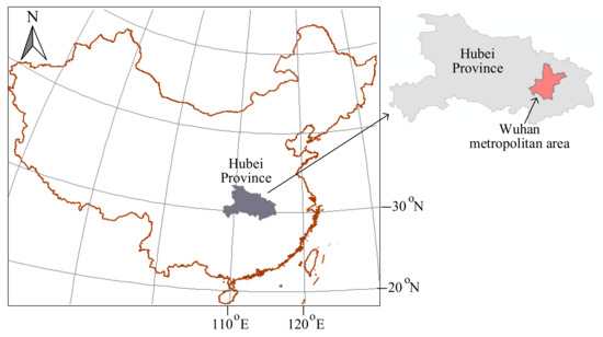
Figure 1.
The study area, Wuhan metropolitan area (WMA), mapped under the cartographic reference system of WGS84.
Urban ecosystem services, particularly from green vegetation cover, are of importance for sustainable urban development in WMA. WMA is one of the 17 cities in the global sustainable development plan issued by the United Nations Development Programme and the United Nations Environment Programme [46]. Vegetation cover in WMA takes multiple forms, including croplands, forestry, street plantation, lawns, parks, gardens, and wetlands. Due to rapid urbanization, a significant part of croplands and forest has been converted into built-up land, which not only reduced the overall vegetated area but also updated the structure in vegetation cover, i.e., increased urban greenness fragmentation. At the same time, the local government has realized the critical consequences from vegetation cover loss and launched several programs to maintain the ecosystem services. For example, afforestation and reforestation have produced positive effect on vegetation restoration [47]. Furthermore, vegetation protection around the water bodies in WMA makes a significant contribution to the urban greenness [48]. So far, the urban greenness fragmentation in WMA has not been systematically studied and modeling its dynamics is valuable to make informed policies for urban development.
Since the objective was to explore vegetation cover fragmentation, all vegetation cover forms in WMA were merged into a single category as vegetated area. The land cover maps of China at 30 m spatial resolution, which are available from China’s data sharing service system (http://data.casearth.cn, accessed on 21 April 2021) [49], were used to compile the vegetated area in WMA. The land cover data have a two-level land type classification schema, including 9 basic land-cover types at level 1 and 22 extended land cover types at level 2 (Table 1), which was one of the most detailed land cover maps freely available [50]. The land cover data include raster maps for the years 2015 and 2020 and were clipped by the boundary of WMA. The land cover types in the clipped maps were aggregated into vegetated areas, water bodies, and urbanized areas using the reclassification schema in Table 1 (Figure 2). The urbanized areas mainly appear in the central part of WMA and also scatter across the region because of dispersed human settlements particularly in the dozens of district centers. The urbanized area increases significantly from 2015 to 2020 while vegetated area reduces accordingly. Further, a digital elevation model (DEM) was used to map the terrain properties. The DEM data, which is the Global Multi-resolution Terrain Elevation Data 2010, have a spatial resolution of about 30 m and were acquired from the United States Geological Survey [51]. Topographic slope was derived from the DEM.

Table 1.
Reclassification schema for the land cover types.
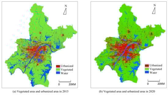
Figure 2.
Urban vegetation cover for the years 2015 and 2020 in Wuhan Metropolitan area.
3. Methodology
3.1. Indicator for Urban Greenness Fragmentation
A newly developed indicator, referred to as Frag, for measuring UVCF was proposed. To compute Frag, land cover is reclassified or resampled as a binary raster map labeled by vegetated and non-vegetated. A square neighborhood window Wmax is predefined to compute the nearest distance between vegetated pixels. For a vegetated pixel Pi, the distance to any other vegetated pixel Pj within Wmax centering at Pi, Disi,j, is defined as,
where is vertical distance between Pi and Pj, is the horizontal distance between pixels, and Disi,j is in pixel unit. Particularly, if Pj shares edge with Pi, then Disi,j will be 1; if Pj shares a vertex with Pi, Disi,j will be ; if there is no satisfied Pj in Wmax, Disi,j takes the maximum distance from the center to the boundary of Wmax. The nearest distance of Pi to its adjacent vegetated area, NDi, is expressed as,
where function Min returns the minimum value from the collection of Disi,j and m is the total number of vegetated pixels excluding Pi in Wmax. In Equation (2), if m = 0 then NDi takes the maximum distance from Pi to the boundary of Wmax; clearly a square-shaped neighborhood window with an odd number of pixels in width for Wmax will result in NDi = × w/2, where w is the size (edge length in pixels) of the window Wmax. Any vegetated pixel having NDi = × w/2 is viewed as having reached the maximum UVCF. Under a given Wmax, a new raster data ND can be derived from the land cover map from Equation (2).
NDi = Min{Disi,j, j = 1, 2, …, m and j ≠ i}
The pattern of resultant Frag is dependent on the analytical scales. A series of scales defined by different sizes of neighborhood windows up to Wmax is tested to check the scale impact on Frag. The newly proposed Frag is designed to reveal scale-dependent UVCF by taking into account both the structure and abundance of vegetation cover. Accordingly, Frag has two parts in its definition. For the first part, the structure of vegetation distribution in a neighborhood (moving) window centered at Pi at scale s, AVG_NDs,i, is defined as the average nearest distance for all the vegetated pixels in the current window, namely,
where NDi represents the nearest distance of Pi to its adjacent vegetated area in the current examined window and nv (nv ≥ 1) is the total number of vegetated pixels in the window. AVG_NDs,i reflects the structure of the vegetated pixels only, through the averaged nearest distance between vegetated pixels within the current neighborhood window at scale s, where s is subject to s ≤ w and w is the maximum scale (edge length in pixels) defined for the window Wmax. However, the percentage or abundance of vegetation cover and the impact of scale on UVCF are not captured in this part. To solve the limitation, the second part considers the percentage of vegetation cover and the scale effect, by computing the average nearest distance of vegetated pixels over the neighborhood window at scale s, or AVG_NDs as,
where n is the total number of pixels in the neighborhood window at scale s. For cases having similar structure in vegetation distribution, i.e., identical AVG_NDs,i, AVG_NDs captures the vegetation cover percentage and scale effect. By combining the two parts together, Frag at scale s takes the form of,
where Frags indicates the averaged nearest distance between vegetated pixels under scale s by considering both the structure and abundance in vegetation cover as well as the analytical scale impact. Figure 3 illustrates a typical example in Frag computation within a window or neighborhood size (s = 5). The nearest distance, NDi, for each vegetated pixel is derived according to Equation (2). The two parts, namely AVG_NDs,i and AVG_NDs, in the Frag definition together provide a comprehensive measurement for UVCF.
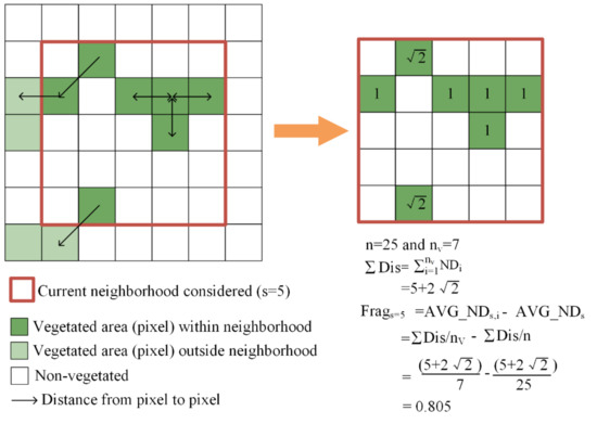
Figure 3.
Example for computing scale-dependent urban greenness fragmentation considering both aggregation structure and abundance of vegetation cover.
3.2. Urban Greenness Fragmentation Modeling by SVM
The Frag indicator enables mapping the pattern changes in urban greenness. Based on the land cover maps in 2015 and 2020, the Frag in the two years were computed to derive Frag changes (Fragdiff) during the period. For any location, three possible Frag change modes were derived from the Frag maps, namely increased Frag, decreased Frag, and unchanged Frag. We are particularly interested in understanding the factors causing the increased and decreased Frag.
Support vector machines (SVMs) have been widely used in classification objectives [52]. To build a SVM model, the input data are grouped into two sets of cases (samples), denoted as positive cases or negative cases, in an n-dimensional space, where n is the number of dimensions or variables. Training a SVM model is to find a separating hyperplane in the n-dimensional space so that the margin between the two sets of cases is maximized. An essential decision is to select a kernel which maps the input vectors (i.e., samples) into a new feature space in which the samples can be linearly separated. Several kernels are available for SVM but radial basis function (RBF) was selected in this study because it is the most popular and resulted in improved accuracy of Goodness-of-Fit than that from other kernels such as Sigmoid kernel and linear Kernel. Detail mathematical description about SVM can be referred to from existing literature [53].
Urban vegetation cover is usually affected by socio-economic activities and natural conditions [54,55,56]. Urbanization transforms vegetated land into urbanized area and fragments vegetation cover [40]. Natural conditions such as terrain characteristics including elevation and slope have been reported to affect vegetation cover and productivity [57]. Though there are other factors, e.g., transportation, human population, and gross domestic production, they could be either correlated to the urbanization or topography, or not readily available at pixel scale. For example, the road network density in WMA was found to spatially correlate to urbanization (result not reported). Thus, for this particular study region, the selection of urbanization, elevation (Elevation), and slope (Slope) could largely indicate the economic development and natural conditions that are associated with the Frag changes.
Several steps are involved in preparing the associated factors and modeling the Frag changes. First, an exploratory analysis found that UVCF was more likely to occur at locations near the newly urbanized area. Thus, distance to urbanization (D2U) for a given location was computed as being the closest distance from the location to the newly urbanized area which was derived by overlaying the land cover maps in 2015 and 2020. Second, D2U, Elevation and Slope were processed as the mean value, respectively, within a neighborhood window defined by the current analytical scale s and taken as input to the SVM model to map Frag increase or decrease. A random sampling schema was decided to select samples from the Fragdiff map. Positive (Frag increase) and negative (Frag decrease) cases were sampled separately. Totally, 5000 points for both the positive and negative cases were randomly sampled from the Fragdiff map. Out of the samples, 60% were used for model training, and the rest were for validation.
Two hyper-parameters, gamma (γ) and C, for SVM with RBF kernel must be optimized to get the best model structure, which were determined by a grid search algorithm [58]. Specifically, the values for γ and C were systematically changed from low to high, by looping through possible combinations of the two parameters. The combination of γ and C achieving the best prediction performance is decided for the model [53].
3.3. Model Performance Evaluation
Confusion matrix was used to evaluate the modeling result. A confusion matrix table is consisted of n × n elements recording relationship between the map classes and reference classes, respectively, where n is the number of classes [59,60]. Overall accuracy (OA) is a generalized index indicating the model performance which is computed as the ratio of the number of correctly classified samples to the total number of samples, as expressed in the following,
where N is the total number of samples, denotes the diagonal element in the confusion matrix, and n is the number of map classes, which is 2 for the SVM model representing a positive class (increased Frag) and a negative class (decreased Frag).
Cohen’s kappa (k) coefficient is a metric that compares an observed accuracy with an expected accuracy (random chance) in the following equation [61],
where Po is the observed agreement between map classes and reference classes which equals to OA. Pe is the expected accuracy taking the form of , where Mi and Ri are the total number of samples of the mapped class i and the referenced class i, respectively.
In addition to OA and kappa, user’s accuracy and producer’s accuracy provide detail accuracy description for the positive and negative cases from user’s and producer’s perspective. Higher user’s accuracy and producer’s accuracy can result in improved OA and k values. User’s accuracy (UA) reveals the ratio of samples which are incorrectly modeled to a known class when they should have been classified as something else, while producer’s accuracy (PA) reflects the ratio of samples mistakenly classified as something else. UA and PA are defined as,
where i can be 1 (positive case) and 0 (negative) for a binary classifier like SVM, and is the number of samples that have been correctly classified as class i in the map set or referenced set.
3.4. Sensitivity Analysis
Sensitivity analysis is often applied to explore the effect of each selected factors for SVM models [62]. To this end, two rounds of modeling analysis were performed. First, SVM model was built to predict the Frag changes (a decreased or increased Frag) based on the set of training samples with input of the selected factors. Next, after updating the values of each variable (factor) of the same samples, i.e., by adding or subtracting by a small amount of value determined from the distribution of the variable values, the built SVM model was used to predict the Frag changes again and the modeled results, i.e., the Frag changes, from the two rounds, i.e., with original and updated input, were compared after the increase or decrease of the input factor. The impact of each selected factor is evaluated separately. Specifically, in the current study 10% of the mean value was added and subtracted on the original value of a factor for all the selected samples, while the input from the others were kept unchanged. Here the mean value of each variable was set as a reference standard because it is meaningful to know how significant a small deviation from the mean value of the variables would update the Frag changes. The number of samples in the model output, namely the positive cases (increased Frag) and negative cases (decreased Frag) in response to the original and updated values of each factor was compared. More samples being predicted to show Frag increase with the increased value from the input variable denote a positive effect on the Frag from the variable and vice versa. The sensitivity analysis was performed for all the scales to test if there was scale effect from the selected factors.
3.5. Computation Platform
Google Earth Engine (GEE) has been increasingly used in environmental and urban studies due to its cloud-based geospatial processing capability and accessibility to a large collection of geospatial datasets [63]. GEE allows to upload local (user’s) data to the user repository and then make integrated analysis by taking both the available platform data resources and analytical tools. For example, the land cover maps in the current study could be uploaded to the user’s repository first, which makes it easier to take advantages of the computing power of GEE and existing algorithms in GEE. Frag computation takes input from the land cover maps for the years 2015 and 2020. D2U was computed from the land cover maps, as explained in Section 3.2. Associated factor analysis using SVM model was made with the input data of the land cover maps, Elevation and Slope. All the analyses, including Frag mapping, SVM modeling, result validation, and sensitivity analysis were performed on GEE.
4. Results
4.1. Spatio-Temporal Changes in Urban Greenness Fragmentation
Considering the spatial scale of the vegetation cover is 30 m, a maximum edge of the neighborhood or window size was defined to be 21 pixels in length, or 10 pixels equivalent of 300 m at each side in regard to any central location. Various window scales, from 3 × 3 up to no higher than the maximum window size, i.e., 21 × 21, were computed. The spatial distribution of urban greenness fragmentation measured by the Frag showed a clear clustering pattern in WMA (Figure 4). The Frag distributions in the years 2015 and 2020 are presented in Figure 4a,b, respectively, with the neighborhood size at 7 × 7. Similar patterns in UVCF were observed at other scales (results not reported). The Frag distribution maps, with high values clustered at the central area and lower values in suburban areas, are largely consistent with reality, suggesting that the indicator Frag serve a good proxy for urban greenness fragmentation. The Frag distribution is closely related to land cover types. The urbanized area, located mainly at the central part of the study area, is characterized by much higher Frag if compared to the suburban areas which are mostly covered by cropland and forestry. Thus, urbanization may promote UVCF in WMA.
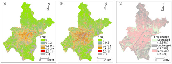
Figure 4.
Spatial distribution and temporal dynamics of the urban greenness fragmentation using Frag indicator. (a) and (b) show vegetation fragmentation (Frag) distribution in 2015 and 2020, respectively and (c) is the vegetation fragmentation (Frag) changes during 2015–2020.
Vegetation cover shows more fragmented in the year 2020 than in 2015, which is revealed by comparing the Frag distribution maps in the two years. Frag changes during the period, including increased, decreased, and unchanged, were derived, as shown in Figure 4c. The increased Frag, reflected by either reduced vegetated area or division of large vegetation patches into smaller pieces, dominated primarily in the newly built-up areas as well as some other areas close to the cropland, covering an area of 42.67% out of the total land. The decreased Frag, a sign of vegetation restoration or improvement, was observed mostly close to rivers and lakes, covering 19.56% of the total area. The improved vegetation cover indicated by the decreased Frag possibly came from strengthened vegetation protection around water bodies, as the local government paid more attention to vegetation’s ecosystem services including the green and blue infrastructure program during those years [64]. Lastly, 37.76% of the study area did not show any change in Frag, which mostly consisted of water bodies where no vegetation was present and forestry where vegetation protection was strictly implemented.
4.2. Modeling the Frag Changes by SVM
An increase or decrease in urban greenness fragmentation, as indicated by the Frag changes during the study period, was modeled by SVM with the selected factors from urbanization and the terrain properties. SVM models show reasonable performance with an overall accuracy ranging between 79.8 and 84.5% and Kappa between 0.61 and 0.69 at different scales defined by neighborhood windows (Figure 5). The model performance is scale dependent and selecting the optimal neighborhood size or scale is important for urban greenness fragmentation modeling. The preferable scales from the model output include 3 × 3, 5 × 5, and 7 × 7. The model accuracy drops when the scale is larger than 7 × 7. The best performance was obtained at 5 × 5 when the highest overall accuracy and Kappa value were obtained, implying that the necessary information from the explanatory variables to predict the Frag increase and decrease was optimally captured at this scale.
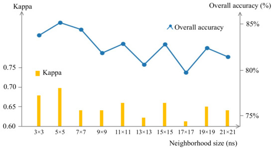
Figure 5.
Scale effect on the performance of modeling the Frag changes.
The variation in the overall accuracy (and Kappa coefficient) comes from the differences in the user’s and producer’s accuracy for the positive (increased Frag) and negative (decreased Frag) cases shown in the confusion matrix (Table 2). For all the scales, the user’s accuracy is higher for the decreased Frag cases than that for the increased ones while the producer’s accuracy presents an opposite result. For example, at the neighborhood size 5 × 5 which achieves the best overall accuracy, the user’s accuracy suggests that, from the user’s perspective, 90% and 80% out of the cases modeled to show decreased and increased Frag were consistent with the reference data, respectively, while the producer’s accuracy suggests that 78% and 92% of the reference data have been correctly produced for the samples that showed decreased and increased Frag, respectively. The relatively lower user’s accuracy of the increased Frag cases than that of the decreased indicates that more cases showing decreased Frag in reference data were mistakenly predicted to be decreased, if compared to the number of the increased Frag cases which were wrongly output as being increased. The higher producer’s accuracy for increased Frag cases suggests that the model performs better for predicting increased Frag cases than decreased. It is noteworthy that for either the decreased or increased Frag from the user’s or producer’s accuracy at the scale 5 × 5, none of the 4 accuracy elements in the confusion matrix is the highest compared to those at other scales; nevertheless, the scale at 5 × 5 shows the most balanced prediction performance in the combination of the user’s and producer’s accuracy and positive and negative cases (decreased and increased Frag), which makes the scale more preferable than the others.
Table 2.
Model performance among different neighborhood sizes.
4.3. Sensitivity Analysis of the Factors on Urban Greenness Fragmentation
The urban greenness fragmentation has been successfully modeled by SVM with the selected variables as input, including the distance to urbanized (D2U), Elevation, and Slope. To further examine the relative importance and direction of the factors’ impact on the Frag changes, a sensitivity analysis was carried out by comparing the model output with the original and updated explanatory variables. Of the three variables, D2U shows the most significant influence to the Frag changes (increase or decrease) during 2015–2020, followed by Elevation and Slope (Figure 6). The negative value (y) showing the percentage of samples that have switched from Frag increase to Frag decrease after a 10% increase of D2U reveals more samples are likely to experience Frag decrease in response to a higher D2U input (Figure 6a). Reversely, more increased Frag cases (a positive y) were output from a 10% decrease of D2U, which suggests that closeness to urbanization increases the likelihood to experiencing Frag increase (Figure 6b). The Elevation shows moderate intensity but in an opposite direction in terms of its impact on the Frag changes, meaning higher elevation promotes UVCF and vice versa. Lastly, Slope presents very slight impact on the Frag changes.
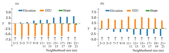
Figure 6.
Sensitivity analysis of urban greenness fragmentation (Frag) to the selected factors. The axis y indicates the percentage of samples (and impact direction) that have switched to Frag increase (positive y) or decrease (negative y) during 2015–2020 in response to updated explanatory x values, i.e., increasing and decreasing 10% from the averaged (x ± meanx), for each variable (D2U, Elevation, or Slope), where meanx is the averaged value of the samples for the variable x (represented in the x axis). A positive y means more samples were observed to show an increase in Frag during 2015–2020 from the model when any explanatory factor (x) increases/decreases by 10%, and vice versa. Note that for each combination in the neighborhood size and 10% increase (a) or decrease (b) of an explanatory factor, the Frag change was found to be in consistent direction (either positive or negative) in response to the x increase or decrease.
The scale, as indicated by different neighborhood sizes (the x axis in Figure 6), alters the impact of the explanatory variables on the Frag changes. The sensitivity of the Frag changes to D2U fluctuates at scales, ranging from −4.0% at the scale 19 × 19 to −6.6% at 5 × 5 in response to increased D2U (Figure 6a) and from 4.0% at the scale 3 × 3 to 6.0% at 11 × 11 in response to the decreased D2U (Figure 6b). The sensitivity of the Frag changes to Elevation largely shows a consistent increase as the scale increases. Slope shows slight impact on the Frag changes at all scales. At smaller scales (e.g., ns ≤ 13 × 13), D2U is the most significant factor on Frag changes, emphasizing the leading effect of urbanization on inducing UVCF, which is consistent with other study [65]. As the scale increases, the impact from Elevation on the Frag changes becomes more obvious. The directions in the Frag changes (y values) in response to the increased or decreased value of the selected factors were unchanged over all the scales, suggesting a robust and consistent impact from all the selected factors (Figure 6).
5. Discussions
5.1. Advantages of Applying Frag in Indicating Urban Greenness Fragmentation
Green vegetation is a key element for supporting ecological services for urban inhabitants. Uncontrolled fragmentation in urban vegetation cover may reduce urban ecological services [66,67]. The spatio-temporal changes in urban greenness fragmentation is one of the key considerations for designing urban policies [68]. Understanding the associated factors of the changes in urban greenness fragmentation is of significance for urban management [27]. Numerous landscape indicators can be taken to map urban greenness fragmentation, varying from simple measures such as number of patches, mean size of the patches, simple edge metrics or patch density to more sophisticated ones in measuring specific fragmentation characteristics such as landscape division, adjacency-based metrics, cohesion, splitting index, Shannon’s diversity, proximity, distance to a patch class, and connectivity [69]. However, to our knowledge, none of the indicators can simultaneously reflect the difference in the structure and abundance in vegetation cover and the impact of analytical scales. The proposed Frag is such an indicator to highlighting varied fragmentation patterns of vegetation cover over space. The Frag indicator can be computed at local scales defined by neighborhood windows and thus the spatial heterogeneity in the fragmentation of vegetation cover is properly illustrated, as shown from the case study (Figure 4). Because urban expansion can easily reduce vegetation cover area and fragment large vegetated area into smaller patches, the proposed Frag indicator measuring both the abundance and aggregation structure in vegetation cover provides a more comprehensive perspective in presenting the spatial distribution patterns and is preferable to study the impact on urban greenness from urbanization.
5.2. Modeling the Associated Factors for the Frag Changes
The current study has adopted SVM to examine the relationship between the selected factors and the Frag changes. There are many models that could be potentially applied to explore the cause-and-effect relationships or associations between variables. These models range from traditional statistics such as regression models and correlation analysis [9,29] to more advanced ones using machine learning approaches [30,34]. SVM is one of the most often applied machine learning models that can classify images from input of explanatory variables [52]. SVM has shown more generalization capacity and less variability in remote sensing image classification compared to neural networks and classification and regression trees [70]. The SVM model in the current study shows a robust result in terms of the overall accuracy (79.8–84.5%) for explaining the Frag changes under all the analytical scales, though similar models are yet to be comprehensively tested. Comprehensive evaluation of various models that best predict the Frag changes will be our next attention.
Previous studies reported that many factors, including urbanization or anthropogenic activities and other natural factors, could be responsible for urban vegetation fragmentation [54,55,56], and models to predict Frag changes and reveal the associated factors of the changes are a helpful step to understand the process of urban greenness fragmentation. The case study suggests that the selected explanatory variables are good for predicting the Frag increase or decrease. The study confirms that urbanization was the most important factor inducing vegetation cover fragmentation, though the elevation and slope also explained the Frag changes. Understanding the contribution of the associated factors of urban vegetation cover fragmentation and the heterogeneity in the spatial distribution of the factors will help in landscape designing, management, and planning [26]. For example, urban development policies should plan vegetation protection measures in urbanized areas, particularly in higher elevation areas which are more prone to urban greenness fragmentation in WMA.
5.3. Further Improvement
The current work proposed a distance-based indicator to map urban greenness fragmentation considering both the abundance and structure of vegetation cover and demonstrated that SVM could be successfully applied to explore the associated factors of the fragmentation changes. Nevertheless, we acknowledge that uncertainties and further improvement from the model deserves future attention.
First, the dependent variable, i.e., the Frag changes, was derived from the existing land cover maps which were classified from remote-sensed images. Our study shows that Frag serves a good indicator to measuring the overall urban greenness fragmentation. However, we did not differentiate the fragmentation of different land cover forms (e.g., croplands, forestry, and street plantation) in the case study. Our purpose in the case study was to explore the urban greenness fragmentation and its associated factors, thus those vegetated land cover forms were combined together to be a single category. It is natural to include only a single land cover class if the fragmentation pattern for that specific type is desired. In addition, though the quality of the data has been extensively verified by various applications, the computation of Frag for the years 2015 and 2020 and the changes in Frag during the period by overlaying the two maps will inevitably introduce and even exaggerate more noise in the dependent variable. Thus, the quality of the data source for computing the Frag indicator has critical impact on the model performance.
Second, there are other factors related to socio-economic activities but urban sprawl has been confirmed to be a key factor for the fragmentation of urban vegetation cover [28,71,72]. Similarly, natural factors were represented by terrain characteristics in the current study, though other factors such as soil class and climatic variables which contribute to vegetation growth were omitted. As an environmental factor, topography can affect distribution and properties in vegetation cover [57,73]. Thus, elevation and slope were included in the SVM model. Our study has shown the Frag indicator could effectively measure urban greenness fragmentation and demonstrated that the Frag changes could be reasonably modeled by SVM with the input of the selected factors. Analysis of the Frag changes taking a full set of variables as mentioned above, however, is out of the scope of this work because pixel-scale datasets such as population density and gross domestic production are not readily available and must be left for future work. Furthermore, it is understandable that the relationship between the Frag changes and the explanatory factors could vary between cities and therefore an exploratory analysis can be useful for optimizing the selection of the factors.
Last but not least, the current study on modeling the urban greenness considers the two-dimensional scope only. There are several studies that have focused on 3D perspective by taking point cloud data and 3D GIS modeling to explore vertical structure in urban vegetation distribution [11,42,43]. Those studies rely on more complicated data collection such as LiDAR sensors and provide a different view on the urban vegetation pattern, which deserves future attention by integrating the 3D data and the proposed Frag modeling.
6. Conclusions
Green vegetation in urbanized area plays a vital role in urban ecosystems. Rapid transformation from vegetated areas into urbanized land has not only reduced vegetated area but also triggered considerable vegetation cover fragmentation, which often exhibits a negative effect to urban ecosystem services. Quantitative measurement of urban greenness fragmentation and understanding its dynamics are highly desired by urban planners. Though various indicators for landscape fragmentation have been developed and applied in mapping vegetation cover fragmentation, the existing ones are limited for the lack of simultaneously taking into account the structure and abundance of vegetation cover. Furthermore, landscape indicators capable of scale-dependent representation are critical for revealing the changes of vegetation cover fragmentation at various scales, which can provide key insight for understanding site-specific impact from the factors on the fragmentation changes in a heterogeneous geographical space.
This study proposed a new distance-based landscape fragmentation metric called Frag to map urban greenness (vegetation cover) fragmentation. The indicator Frag can highlight both the structure and abundance in vegetation cover that vary over space. The proposed Frag represents vegetation cover fragmentation from two aspects. First, the structure, or aggregation pattern, in vegetation cover is measured by the average nearest distance (AND) between the vegetated pixels (see Equation (3)). A larger AND between the vegetated pixels suggests more fragmented vegetation cover and vice versa. Second, the percentage or abundance in vegetation cover is measured by the AND over the whole area of the neighborhood window which defines the analytical scale (see Equation (4)). By combining the two together (Equation (5)), Frag can serve as an objective indicator to mapping urban greenness fragmentation.
The study applied SVM to understand the impact on the Frag changes from urbanization and terrain characteristics. The modeling results indicate that the Frag changes could be reasonably explained by the selected factors. The case study in WMA demonstrates that urbanization was the most sensitive factor that induced vegetation cover fragmentation during the study period. Because urban greenness fragmentation from both the structure and abundance in vegetation cover could be effectively measured by Frag and the Frag changes be explained by cause-effect models such as SVM, it is possible to project the trajectory of Frag for the future, which provides valuable references for urban planning.
Author Contributions
Conceptualization, Zongyao Sha and Husheng Fang; methodology, Husheng Fang; software, Husheng Fang and Moquan Sha; validation, Dai Qiu, Wenjuan Lin and Moquan Sha; formal analysis, Husheng Fang; investigation, Zongyao Sha; writing—original draft preparation, Husheng Fang; writing—review and editing, Zongyao Sha; visualization, Husheng Fang; funding acquisition, Zongyao Sha. All authors have read and agreed to the published version of the manuscript.
Funding
This research was funded by the National Natural Science Foundation of China grant number 41871296.
Institutional Review Board Statement
Not applicable.
Data Availability Statement
Publicly available datasets were analyzed in this study. The data can be found here: http://data.casearth.cn, accessed on 21 April 2021.
Conflicts of Interest
The authors declare no conflict of interest.
Nomenclature
| WMA | Wuhan Metropolitan Area |
| UVCF | Urban Vegetation Cover Fragmentation |
| SVM | Support Vector Machine |
| NNI | Nearest Neighbor Index |
| AI | Aggregation Index |
| D2U | Distance to Urbanization |
| OA | Overall Accuracy |
References
- Liu, Z.; He, C.; Wu, J. General Spatiotemporal Patterns of Urbanization: An Examination of 16 World Cities. Sustainability 2016, 8, 41. [Google Scholar] [CrossRef] [Green Version]
- Cao, H.; Liu, J.; Fu, C.; Zhang, W.; Wang, G.; Yang, G.; Luo, L. Urban Expansion and Its Impact on the Land Use Pattern in Xishuangbanna since the Reform and Opening up of China. Remote Sens. 2017, 9, 137. [Google Scholar] [CrossRef] [Green Version]
- Li, X.; Song, J.; Lin, T.; Dixon, J.; Zhang, G.; Ye, H. Urbanization and health in China, thinking at the national, local and individual levels. Environ. Health 2016, 15, S32. [Google Scholar] [CrossRef] [Green Version]
- He, C.; Liu, Z.; Xu, M.; Ma, Q.; Dou, Y. Urban expansion brought stress to food security in China: Evidence from decreased cropland net primary productivity. Sci. Total Environ. 2017, 576, 660–670. [Google Scholar] [CrossRef] [PubMed]
- Guan, X.; Shen, H.; Li, X.; Gan, W.; Zhang, L. A long-term and comprehensive assessment of the urbanization-induced impacts on vegetation net primary productivity. Sci. Total Environ. 2019, 669, 342–352. [Google Scholar] [CrossRef] [PubMed]
- Imhoff, M.L.; Bounoua, L.; DeFries, R.; Lawrence, W.T.; Stutzer, D.; Tucker, C.J.; Ricketts, T. The consequences of urban land transformation on net primary productivity in the United States. Remote Sens. Environ. 2004, 89, 434–443. [Google Scholar] [CrossRef]
- Li, X.; Zhou, Y.; Asrar, G.R.; Mao, J.; Li, X.; Li, W. Response of vegetation phenology to urbanization in the conterminous United States. Glob. Chang. Biol. 2016, 23, 2818–2830. [Google Scholar] [CrossRef]
- Zhao, S.; Liu, S.; Zhou, D. Prevalent vegetation growth enhancement in urban environment. Proc. Natl. Acad. Sci. USA 2016, 113, 6313–6318. [Google Scholar] [CrossRef] [Green Version]
- Gui, X.; Wang, L.; Yao, R.; Yu, D.; Li, C. Investigating the urbanization process and its impact on vegetation change and urban heat island in Wuhan, China. Environ. Sci. Pollut. Res. 2019, 26, 30808–30825. [Google Scholar] [CrossRef]
- Santos, T.; Tenedório, J.A.; Gonçalves, J.A. Quantifying the City’s Green Area Potential Gain Using Remote Sensing Data. Sustainability 2016, 8, 1247. [Google Scholar] [CrossRef] [Green Version]
- Santos, T.; Silva, C.; Tenedório, J.A.; Montenegro Góes, T. Remote Sensing and GIS for Modelling Green Roofs Potential at Different Urban Scales. In Methods and Applications of Geospatial Technology in Sustainable Urbanism; IGI Global: Hershey, PA, USA, 2021; pp. 251–293. ISBN 9781799822493. [Google Scholar]
- Zambrano, L.; Aronson, M.F.J.; Fernandez, T. The Consequences of Landscape Fragmentation on Socio-Ecological Patterns in a Rapidly Developing Urban Area: A Case Study of the National Autonomous University of Mexico. Front. Environ. Sci. 2019, 7, 152. [Google Scholar] [CrossRef]
- Collinge, S.K. Ecological consequences of habitat fragmentation: Implications for landscape architecture and planning. Landsc. Urban Plan. 1996, 36, 59–77. [Google Scholar] [CrossRef]
- McGarigal, K.; Cushman, S.A.; Ene, E. FRAGSTATS V. 4. Spatial Pattern Analysis Program for Categorical and Continuous Maps. Available online: http://www.umass.edu/landeco/research/fragstats/fragstats.html (accessed on 20 September 2012).
- Pommerening, A.; Szmyt, J.; Zhang, G. A new nearest-neighbour index for monitoring spatial size diversity: The hyperbolic tangent index. Ecol. Model. 2020, 435, 109232. [Google Scholar] [CrossRef]
- Ferreira, L.M.R.; Esteves, L.S.; de Souza, E.P.; dos Santos, C.A.C. Impact of the Urbanisation Process in the Availability of Ecosystem Services in a Tropical Ecotone Area. Ecosystems 2018, 22, 266–282. [Google Scholar] [CrossRef] [Green Version]
- Chen, T.; Niu, R.-Q.; Wang, Y.; Zhang, L.-P.; Du, B. Percentage of Vegetation Cover Change Monitoring in Wuhan Region Based on Remote Sensing. Procedia Environ. Sci. 2011, 10, 1466–1472. [Google Scholar] [CrossRef] [Green Version]
- Li, B.-L.; Archer, S. Weighted mean patch size: A robust index for quantifying landscape structure PII S 0 3 0 4-3 8 0 0. Ecol. Model. 1997, 102, 353–361. [Google Scholar] [CrossRef]
- Hamad, R.; Kolo, K.; Balzter, H. Post-War Land Cover Changes and Fragmentation in Halgurd Sakran National Park (HSNP), Kurdistan Region of Iraq. Land 2018, 7, 38. [Google Scholar] [CrossRef] [Green Version]
- Zhou, W.; Wang, J.; Qian, Y.; Pickett, S.T.A.; Li, W.; Han, L. The rapid but “invisible” changes in urban greenspace: A com-parative study of nine Chinese cities. Sci. Total Environ. 2018, 627, 1572–1584. [Google Scholar] [CrossRef]
- Khalyani, A.H.; Mayer, A.; Webster, C.R.; Falkowski, M.J. Ecological indicators for protection impact assessment at two scales in the Bozin and Marakhil protected area, Iran. Ecol. Indic. 2013, 25, 99–107. [Google Scholar] [CrossRef]
- Šímová, P.; Gdulová, K. Landscape indices behavior: A review of scale effects. Appl. Geogr. 2012, 34, 385–394. [Google Scholar] [CrossRef]
- Yang, J.; Li, S.; Xu, J.; Wang, X.; Zhang, X. Effects of changing scales on landscape patterns and spatial modeling under ur-banization. J. Environ. Eng. Landsc. Manag. 2020, 28, 62–73. [Google Scholar] [CrossRef]
- Sowińska-Świerkosz, B.; Michalik-Śnieżek, M. The Methodology of Landscape Quality (LQ) Indicators Analysis Based on Remote Sensing Data: Polish National Parks Case Study. Sustainability 2020, 12, 2810. [Google Scholar] [CrossRef] [Green Version]
- Threlfall, C.G.; Ossola, A.; Hahs, A.K.; Williams, N.S.G.; Wilson, L.; Livesley, S.J. Variation in Vegetation Structure and Composition across Urban Green Space Types. Front. Ecol. Evol. 2016, 4. [Google Scholar] [CrossRef] [Green Version]
- Dronova, I. Environmental heterogeneity as a bridge between ecosystem service and visual quality objectives in management, planning and design. Landsc. Urban Plan. 2017, 163, 90–106. [Google Scholar] [CrossRef]
- Yang, C.; Li, R.; Sha, Z. Exploring the Dynamics of Urban Greenness Space and Their Driving Factors Using Geographically Weighted Regression: A Case Study in Wuhan Metropolis, China. Land 2020, 9, 500. [Google Scholar] [CrossRef]
- Du, J.; Fu, Q.; Fang, S.; Wu, J.; He, P.; Quan, Z. Effects of rapid urbanization on vegetation cover in the metropolises of China over the last four decades. Ecol. Indic. 2019, 107, 105458. [Google Scholar] [CrossRef]
- Aguilar, R.; Cristóbal-Pérez, E.J.; Balvino-Olvera, F.J.; Aguilar-Aguilar, M.; Aguirre-Acosta, N.; Ashworth, L.; Lobo, J.A.; Martén-Rodríguez, S.; Fuchs, E.J.; Sanchez-Montoya, G.; et al. Habitat fragmentation reduces plant progeny quality: A global synthesis. Ecol. Lett. 2019, 22, 1163–1173. [Google Scholar] [CrossRef] [Green Version]
- Brown, M.E.; Lary, D.J.; Vrieling, A.; Stathakis, D.; Mussa, H. Neural networks as a tool for constructing continuous NDVI time series from AVHRR and MODIS. Int. J. Remote Sens. 2008, 29, 7141–7158. [Google Scholar] [CrossRef] [Green Version]
- Balzter, H. Markov chain models for vegetation dynamics. Ecol. Model. 2000, 126, 139–154. [Google Scholar] [CrossRef] [Green Version]
- Li, S.; Hartemink, N.; Speybroeck, N.; Vanwambeke, S.O. Consequences of landscape fragmentation on Lyme disease risk: A cellular automata approach. PLoS ONE 2012, 7, e39612. [Google Scholar] [CrossRef] [PubMed] [Green Version]
- Mirbagheri, B.; Alimohammadi, A. Integration of Local and Global Support Vector Machines to Improve Urban Growth Modelling. ISPRS Int. J. Geo-Inf. 2018, 7, 347. [Google Scholar] [CrossRef] [Green Version]
- Keshtkar, H.; Voigt, W. A spatiotemporal analysis of landscape change using an integrated Markov chain and cellular au-tomata models. Model. Earth Syst. Environ. 2015, 2, 1–13. [Google Scholar]
- Carter, S.K.; Burris, L.E.; Domschke, C.T.; Garman, S.L.; Haby, T.; Harms, B.R.; Kachergis, E.; Litschert, S.E.; Miller, K.H. Identifying Policy-relevant Indicators for Assessing Landscape Vegetation Patterns to Inform Planning and Management on Multiple-use Public Lands. Environ. Manag. 2021, 68, 426–443. [Google Scholar] [CrossRef]
- Nong, D.H.; Lepczyk, C.A.; Miura, T.; Fox, J.M. Quantifying urban growth patterns in Hanoi using landscape expansion modes and time series spatial metrics. PLoS ONE 2018, 13, e0196940. [Google Scholar] [CrossRef] [Green Version]
- de la Barrera, F.; Henríquez, C. Vegetation cover change in growing urban agglomerations in Chile. Ecol. Indic. 2017, 81, 265–273. [Google Scholar] [CrossRef]
- Zhou, D.; Tian, Y.; Jiang, G. Spatio-temporal investigation of the interactive relationship between urbanization and ecosystem services: Case study of the Jingjinji urban agglomeration, China. Ecol. Indic. 2018, 95, 152–164. [Google Scholar] [CrossRef]
- Bogaert, J.; Barima, Y.S.S.; Mongo, L.I.W.; Bamba, I.; Mama, A.; Toyi, M.; Lafortezza, R. Forest Fragmentation: Causes, Eco-logical Impacts and Implications for Landscape Management. In Landscape Ecology in Forest Management and Conservation; Springer: Berlin/Heidelberg, Germany, 2011; pp. 273–296. [Google Scholar]
- Paul, S.; Nagendra, H. Vegetation change and fragmentation in the mega city of Delhi: Mapping 25 years of change. Appl. Geogr. 2015, 58, 153–166. [Google Scholar] [CrossRef]
- Tenedório, J.A.; Rebelo, C.; Estanqueiro, R.; Henriques, C.D.; Marques, L.; Gonçalves, J.A. New Developments in Geographical Information Technology for Urban and Spatial Planning. In Technologies for Urban and Spatial Planning: Virtual Cities and Territories; IGI Global: Hershey, PA, USA, 2013; pp. 196–227. ISBN 9781466643505. [Google Scholar]
- Magarotto, M.G.; da Costa, M.F.; Tenedório, J.A.; Silva, C.P. Vertical growth in a coastal city: An analysis of Boa Viagem (Recife, Brazil). J. Coast. Conserv. 2015, 20, 31–42. [Google Scholar] [CrossRef]
- Magarotto, M.; Costa, M.F.; Tenedório, J.A.; Silva, C.P.; Pontes, T.L.M. Methodology for the development of 3D GIS models in the Coastal Zone. J. Coast. Res. 2014, 70, 479–484. [Google Scholar] [CrossRef]
- Ding, L.; Zhao, W.; Huang, Y.; Cheng, S.; Liu, C. Research on the Coupling Coordination Relationship between Urbanization and the Air Environment: A Case Study of the Area of Wuhan. Atmosphere 2015, 6, 1539–1558. [Google Scholar] [CrossRef] [Green Version]
- Hu, S.; Tong, L.; Frazier, A.E.; Liu, Y. Urban boundary extraction and sprawl analysis using Landsat images: A case study in Wuhan, China. Habitat Int. 2015, 47, 183–195. [Google Scholar] [CrossRef]
- He, Q.; Tan, R.; Gao, Y.; Zhang, M.; Xie, P.; Liu, Y. Modeling urban growth boundary based on the evaluation of the extension potential: A case study of Wuhan city in China. Habitat Int. 2018, 72, 57–65. [Google Scholar] [CrossRef]
- Feng, J.; Xu, X.; Wu, J.; Zhang, Q.; Zhang, D.; Li, Q.; Long, C.; Chen, Q.; Chen, J.; Cheng, X. Inhibited enzyme activities in soil macroaggregates contribute to enhanced soil carbon sequestration under afforestation in central China. Sci. Total Environ. 2018, 640–641, 653–661. [Google Scholar] [CrossRef]
- Sha, Z.; Ali, Y.; Wang, Y.; Chen, J.; Tan, X.; Li, R. Mapping the Changes in Urban Greenness Based on Localized Spatial Association Analysis under Temporal Context Using MODIS Data. ISPRS Int. J. Geo-Inf. 2018, 7, 407. [Google Scholar] [CrossRef] [Green Version]
- Zhang, X.; Liu, L.; Wu, C.; Chen, X.; Gao, Y.; Xie, S.; Zhang, B. Development of a global 30-m impervious surface map using multi-source and multi-temporal remote sensing datasets with the Google Earth Engine platform. Earth Syst. Sci. Data Discuss. 2020, 3505079, 1–27. [Google Scholar]
- Zhang, X.; Liu, L.; Chen, X.; Xie, S.; Gao, Y. Fine Land-Cover Mapping in China Using Landsat Datacube and an Operational SPECLib-Based Approach. Remote Sens. 2019, 11, 1056. [Google Scholar] [CrossRef] [Green Version]
- Danielson, J.J.; Gesch, D.B. Global Multi-Resolution Terrain Elevation Data 2010 (GMTED2010); USGS: Reston, VA, USA, 2011; Volume 2010, p. 26. [Google Scholar]
- Pal, M.; Maxwell, A.E.; Warner, T.A. Kernel-based extreme learning machine for remote-sensing image classification. Remote Sens. Lett. 2013, 4, 853–862. [Google Scholar] [CrossRef]
- Sha, Z.; Bai, Y. Mapping grassland vegetation cover based on Support Vector Machine and association rules. In Proceedings of the 2013 Ninth International Conference on Natural Computation (ICNC), Shenyang, China, 23–25 July 2013; pp. 44–49. [Google Scholar]
- Yang, K.; Pan, M.; Luo, Y.; Chen, K.; Zhao, Y.; Zhou, X. A time-series analysis of urbanization-induced impervious surface area extent in the Dianchi Lake watershed from 1988–2017. Int. J. Remote Sens. 2018, 40, 573–592. [Google Scholar] [CrossRef]
- Cheptou, P.O.; Hargreaves, A.L.; Bonte, D.; Jacquemyn, H. Adaptation to fragmentation: Evolutionarydynamics driven by human influences. Philos. Trans. R. Soc. B Biol. Sci. 2017, 372, 20160037. [Google Scholar] [CrossRef] [Green Version]
- Luo, Y.; Wu, J.; Wang, X.; Wang, Z.; Zhao, Y. Can policy maintain habitat connectivity under landscape fragmentation? A case study of Shenzhen, China. Sci. Total Environ. 2020, 715, 136829. [Google Scholar] [CrossRef] [PubMed]
- Liu, D.L.; Zhang, Y.S.; Lin, N. Association Analysis of NDVI Changes and Topographic Factors. Appl. Mech. Mater. 2013, 333–335, 1205–1208. [Google Scholar] [CrossRef]
- Syarif, I.; Prugel-Bennett, A.; Wills, G. SVM Parameter Optimization using Grid Search and Genetic Algorithm to Improve Classification Performance. TELKOMNIKA Telecommun. Comput. Electron. Control 2016, 14, 1502. [Google Scholar] [CrossRef]
- Usman, B. Elixir Satellite Imagery Land Cover Classification using K-Means Clustering Algorithm Computer Vision for En-vironmental Information Extraction. Sci. Eng. 2013, 63, 18671–18675. [Google Scholar]
- Landis, J.R.; Koch, G.G. The measurement of observer agreement for categorical data. Biometrics 1977, 33, 159. [Google Scholar] [CrossRef] [Green Version]
- Ben-David, A. About the relationship between ROC curves and Cohen’s kappa. Eng. Appl. Artif. Intell. 2008, 21, 874–882. [Google Scholar] [CrossRef]
- Su, J.; Wang, X.; Zhao, S.; Chen, B.; Li, C.; Yang, Z. A Structurally Simplified Hybrid Model of Genetic Algorithm and Support Vector Machine for Prediction of Chlorophyll a in Reservoirs. Water 2015, 7, 1610–1627. [Google Scholar] [CrossRef] [Green Version]
- Liang, J.; Xie, Y.; Sha, Z.; Zhou, A. Computers, Environment and Urban Systems Modeling urban growth sustainability in the cloud by augmenting Google Earth Engine (GEE). Comput. Environ. Urban. Syst. 2020, 84, 101542. [Google Scholar] [CrossRef]
- Jia, J.; Zhang, X. A human-scale investigation into economic benefits of urban green and blue infrastructure based on big data and machine learning: A case study of Wuhan. J. Clean. Prod. 2021, 316, 128321. [Google Scholar] [CrossRef]
- Jiao, L.; Xu, G.; Xiao, F.; Liu, Y.; Zhang, B. Analyzing the Impacts of Urban Expansion on Green Fragmentation Using Con-straint Gradient Analysis. Prof. Geogr. 2017, 69, 553–566. [Google Scholar] [CrossRef]
- Kiss, T.; Ecseri, K.; Hoyk, E. Ecological services of green areas in the main square of Kecskemét. Gradus 2020, 7, 173–178. [Google Scholar] [CrossRef]
- Li, Z.; Chen, D.; Cai, S.; Che, S. The ecological services of plant communities in parks for climate control and recreation—A case study in Shanghai, China. PLoS ONE 2018, 13, e0196445. [Google Scholar] [CrossRef] [Green Version]
- Dong, Y.; Liu, H.; Zheng, T. Does the Connectivity of Urban Public Green Space Promote Its Use? An Empirical Study of Wuhan. Int. J. Environ. Res. Public Health 2020, 17, 297. [Google Scholar] [CrossRef] [Green Version]
- Llauss, A.; Nogué, J. Indicators of landscape fragmentation: The case for combining ecological indices and the perceptive approach. Ecol. Indic. 2012, 15, 85–91. [Google Scholar] [CrossRef]
- Shao, Y.; Lunetta, R.S. Comparison of support vector machine, neural network, and CART algorithms for the land-cover classification using limited training data points. ISPRS J. Photogramm. Remote Sens. 2012, 70, 78–87. [Google Scholar] [CrossRef]
- Liu, Y.; Wang, Y.; Peng, J.; Du, Y.; Liu, X.; Li, S.; Zhang, D. Correlations between Urbanization and Vegetation Degradation across the World’s Metropolises Using DMSP/OLS Nighttime Light Data. Remote Sens. 2015, 7, 2067–2088. [Google Scholar] [CrossRef] [Green Version]
- Li, D.; Wu, S.; Liang, Z.; Li, S. The impacts of urbanization and climate change on urban vegetation dynamics in China. Urban For. Urban Green. 2020, 54, 126764. [Google Scholar] [CrossRef]
- Deng, S.-F.; Yang, T.-B.; Zeng, B.; Zhu, X.-F.; Xu, H.-J. jie Vegetation cover variation in the Qilian Mountains and its response to climate change in 2000–2011. J. Mt. Sci. 2013, 10, 1050–1062. [Google Scholar] [CrossRef]
Publisher’s Note: MDPI stays neutral with regard to jurisdictional claims in published maps and institutional affiliations. |
© 2021 by the authors. Licensee MDPI, Basel, Switzerland. This article is an open access article distributed under the terms and conditions of the Creative Commons Attribution (CC BY) license (https://creativecommons.org/licenses/by/4.0/).