Visualizing Large-Scale Building Information Modeling Models within Indoor and Outdoor Environments Using a Semantics-Based Method

Abstract

Building information modeling (BIM), with detailed geometry and semantics of the indoor environment, has become an essential part of smart city development and city information modeling (CIM). However, visualizing large-scale BIM models within geographic information systems (GIS), such as virtual globes, remains a technological challenge with limited hardware resources. Previous methods generally removed indoor features in a single-source (BIM) scene to reduce the computational burden from outdoor views, which have not been applied to the multi-source and -scale geographic environment (e.g., virtual globes). This approach neglected special BIM semantics (e.g., transparent windows), which may miss a part of geographic features or buildings and cause unreasonable visualization. Besides, the method overlooked indoor visualization optimization, which may burden computing resources when visualizing big and complex buildings from indoor views. To address these problems, we propose a semantics-based method for visualizing large-scale BIM models within indoor and outdoor environments. First, we organize large-scale BIM models based on a latitude-longitude grid (LLG) in the outdoor environment; a multilayer cell-and-portal graph is used to index the structure of the BIM model and building entities. Second, we propose a scheduling algorithm to achieve the integrated visualization in indoor and outdoor environments considering BIM semantics. The application of the proposed method to a multi-scale and -source environment confirmed that it can achieve an effective and efficient visualization for huge BIM models in indoor-outdoor scenes. Compared with the previous study, the proposed method considers the BIM semantics and thus can visualize more complete features from outdoor and indoor views of BIM models in the virtual globe. Besides, the study only loads as visible data as possible, which can retain lower the volume of increased geometry, and thus keep a higher frame rate for the tested areas.

1. Introduction

The integration of building information modeling (BIM) and geographic information systems (GIS) has become a research focus [1,2,3]. Visualization lays the foundation of BIM-GIS integration, and is necessary for fields such as indoor/outdoor route analysis and navigation [4,5,6], three-dimensional (3D) cadaster [7,8,9], and urban environment analysis [10,11].

In recent years, there has been a considerable research focus on integrated BIM-GIS visualization, which includes two main steps: data organization and scheduling optimization. Previous studies have mainly discussed index structures in single-source (BIM-only) scenes for data organization. For example, Varduhn et al. (2011) organized large-scale BIM using an octree index structure. Liu et al. (2016) proposed a sparse voxelization method to generate a scene index structure concerning large-scale BIM models; their method mainly indexes buildings’ exterior products and interior products with pre-calculated voxel size, which adapts to a single-scale environment. However, 3D GIS (e.g., virtual globes) involves geographic environments constructed using multi-scale data (e.g., terrain, satellite imagery, and 3D city models), which are organized using discrete global grids for efficient processing and visualization [12,13]. Previous studies focused on visualizing single or a few BIM models in the 3D GIS (i.e., virtual globes) based on local index-structures [14,15].

Besides, there are significant technological challenges when applying a large number of BIM models to the geographic environment with limited hardware resources. Previous studies have generally reduced geometric data by mesh simplification or by conversion to lower level of detail (LOD) models [16,17]. However, these approaches can change topological relationships between indoor spaces and the geometric accuracy of the building [18]. To address this issue, some studies have extracted exterior entities from BIM models, which can dynamically reduce geometric information by removing non-exterior entities from outdoor views. Moreover, when entering into the indoor space, it is possible to load indoor entities and even remove other BIM models from outdoor scenes [18,19]. However, previous algorithms face the following two problems. First, current methods directly remove occluded features and neglect special BIM semantics (e.g., transparent window or open door), which may lose some geographical features. Specifically, previous methods cannot observe complete outdoor scenes near windows from indoor views, and cannot see complete indoor information near windows from outdoor views, which causes an unreasonable roaming process and limits the spatial analysis and application in the smart city. For example, a previous study lost a part of exterior building features, and thus could not support solar radiation and lighting analysis (such as the interior solar shading analysis) in the green building [20]. Second, the algorithms explicitly did not focus on the visualization optimization in the indoor space further, which may have heavy hardware resources when loading large and complex indoor buildings from indoor views. Therefore, we noticed that the indoor environment can be divided into multiple enclosed spaces, and other invisible indoor spaces (e.g., rooms) removed by the current location of the indoor view would efficiently reduce data volume.

In this study, we developed a semantics-based method for visualizing large-scale BIM within the indoor-outdoor geographic environment. First, we created a hybrid index to better organize large-scale BIM models: On one hand, we employed LOD strategy and longitude-latitude grid (LLG)-based spatial index to organize large-scale BIM models, which adapt to the virtual globe [21]. On other hand, according to the data structure of the BIM model, we took a multilayer cell-and-portal graph index each space and entities inside the BIM model. Second, we proposed a semantic-based scheduling algorithm for indoor/outdoor scenes to achieve the integrated visualization in indoor and outdoor environments (multi-source and -scale environments). The algorithm can easily and rapidly judge the indoor/outdoor environment by BIM semantics (i.e., indoor space named IfcSpace). Then it can observe realistic indoor-outdoor environments from “visibility” entities (such as a transparent window or open door) and retain a lower computing burden by taking out-of-core rendering technology to reduce the burden, combined with the proposed hybrid index and view-frustum culling.

2. Related Work

2.1. Data Organization for Visualizing Building Information Modeling (BIM) Models in Three-Dimensional Geographic Information Systems (3D GIS)

2.1.1. Level of Detail (LOD)-Based Data Organization

Previous studies have mainly converted BIM models into CityGML models by establishing relationships between BIM in the Industry Foundation Classes (IFC) format and CityGML [22,23,24]. However, LOD models in CityGML employ a discrete LOD strategy; lower LOD models require geometric simplification of the original model and thus lose geometric accuracy. Besides, Xu et al. (2020) organized four LOD models according to the building type, which retains the geometric accuracy of each building entity. However, such strategies focus on the organization of individual BIM models and neglect the organization of the building entities from the perspective of indoor visualization.

2.1.2. Index-Based Data Organization

Compared with LOD-based data organization, index-based data organization can index fine-grained building elements or spatial structures of BIM models. For example, Varduhn et al. (2011) employed an octree index for large-scale BIM models for positioning and dynamic scheduling in huge scenes. However, this approach neglects possible indoor structures of the building. Therefore, Liu et al. (2016) proposed a double-layered sparse voxel (DLSV) structure for data indexing, which mainly uses sparse voxelization by setting a fixed voxel size to build the scene index without any loss of scene detail. This method essentially indexes exterior and interior products separately to organize indoor-outdoor scenes. However, this method only separates the building into indoor and outdoor parts, but lacks the further subdivision of indoor spaces. As such, this strategy may overburden limited hardware resources for loading large and complex indoor buildings.

Moreover, ArcGIS and Cesium can support large-scale BIM models visualization by converting IFC data into specific tree-index in specific data formats such as Indexed 3D Scene Layer(I3S) and 3DTiles [15,25]. However, relevant methods focused on visualizing single or a few BIM models in the virtual globe by local tree-index structures.

Therefore, we created a hybrid index to better organize large-scale BIM models: On the one hand, we employed LOD strategy and LLG-based spatial index to organize large-scale BIM models. In particular, LLG-based spatial index (a global index-structure used by mainstream virtual globe platforms) can give each extent global coding for each level, extra BIM models can easily fuse into the 3D GIS. On the other hand, according to the data structure of the BIM model, we took a multilayer cell-and-portal graph index each space and entity inside the BIM model, which further is subdivided into indoor spaces.

2.2. BIM-Based Scheduling Algorithm for Indoor and Outdoor Scenes

BIM-based scheduling algorithms for indoor and outdoor scenes can be separated into LOD-based scheduling algorithms and index-based scheduling algorithms.

2.2.1. LOD-Based Scheduling Algorithms

Using LOD-based organization, these algorithms can dynamically select and load an appropriate LOD model according to the distance between the viewpoint and the model center. There are two possible approaches, discrete and continuous LOD-based scheduling algorithms. However, in general, these approaches lack optimization strategies for the indoor structure of the BIM model. As such, it is not possible to significantly reduce the computing burden for BIM models with complex indoor structures and a large volume of geometric data. On this basis, this approach cannot efficiently meet the demand for indoor visualization.

2.2.2. Index-Based Scheduling Algorithms

In index-based data organization, algorithms can dynamically load building entities based on viewpoint distance and visible range. For example, a previous study dynamically loaded the BIM model based on an octree index structure neglecting indoor structures [26]. Generally, progressively loading a building’s exterior products from outdoor views. But when roaming into indoor space, the whole product of building would be loaded, which may increase the burden of hardware. Therefore, Liu et al. (2016) proposed a scheduling algorithm called Incremental Frustum of Interest (I-FOI) based on DLSV to progressively load a building’s exterior products from outdoor views, to load indoor products, and to remove other BIM models from indoor scenes. However, the previous algorithm simply eliminated the invisible entities and ignored BIM semantics (such as translucent windows), which may cause unreasonable BIM-GIS visualization especially of an indoor environment. For example, other BIM models are removed directly from indoor views, and realistic and complete scenes near windows cannot be observed. When observing the interior space from outdoor views, the indoor entities cannot be loaded. Undoubtedly, this approach limits the subsequent analysis and application. For example, the previous methods cannot support the solar radiation and lighting analysis, because of the lack of interior and exterior building entities [20]. Moreover, previous research neglected the indoor visualization optimization, and explicitly did not unload other spaces (e.g., rooms) by the current location of the indoor space, which would increase the computing burden for loading big and complex buildings.

Therefore, we propose a semantics-based method for visualizing large-scale BIM models within indoor and outdoor environments. This study decreases the computing burden in the indoor and outdoor views, improve the realistic features, which can lay the foundation of analysis and application. For example, the proposed method can easily provide related building features from indoor and outdoor views, and thus can easily support solar radiation and lighting analysis (such as interior and exterior solar shading analysis) in the green building.

3. Materials and Methods

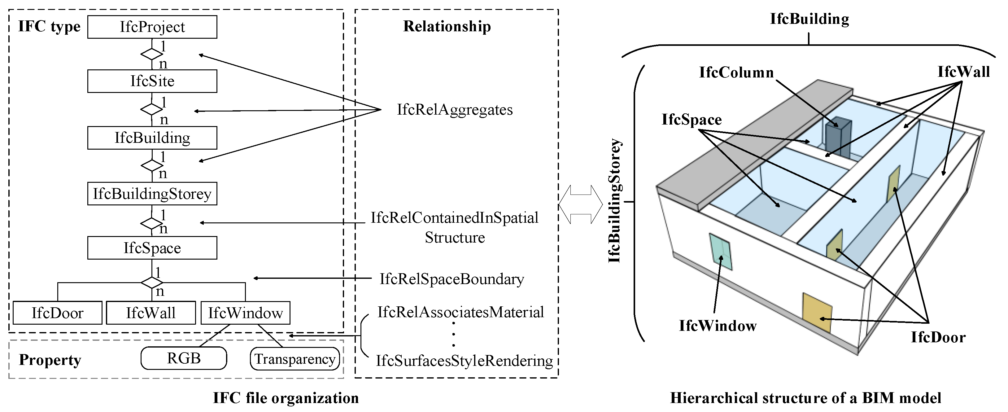
3.1. BIM Semantics

BIM semantics mainly describe architectural details (more than 600 definitions of building entities and 300 definitions of component types) and semantic connections between various building entities [14,27]. As seen in Figure 1, a hierarchical project structure defined by BIM/IFC comprises a well-defined set of semantic information, which includes basic building entities (e.g., IfcProject, IfcSite, IfcBuilding, IfcBuildingStorey) and the relationship called IfcRelAggregates. IfcWindow is associated with properties such as color and transparency via IfcSurfacStyleRendering and other semantics. A detailed description can be found in the IFC4 standard [28].

For a better explanation, we define the term “visibility” based on BIM semantics. And the term “visibility” represents portal entities and relevant attributes affecting the visible range of viewpoints in the building. Specifically, when “visibility” is true, the building type is a portal entity, and spaces connected by the portal are visible to each other (e.g., the opening-closing state of the door is open;

Table 1. Definition of “visibility”.

Class	IFC Type	Description
Portal entity	IfcDoor	Door
	IfcWindow	Window
	IfcStair	Stair
Property	IfcSurfaceStyleShading	Transparency (value between 0 and 1)
	IfcSurfaceStyleRendering	Transparency (value between 0 and 1)
	IfcProperty	Custom property (e.g., opening-closing state of door)

).

3.2. Semantic-Based Data Organization for Large-Scale BIM Models in 3D GIS

We investigated semantic data organization for large-scale BIM models in 3D GIS. Previously, georeferencing has linked local coordinates inside the BIM model with corresponding real-world coordinates, by which a single building or construction is placed within the geographical environment [29,30,31,32]. However, to address the technological challenge of visualizing large-scale BIM models in indoor/outdoor GIS with limited computing resources, we proposed a two-part data organization approach. For the indoor space, we refined the BIM model to construct an index structure (i.e., multilayer cell-and-portal graph) according to BIM/IFC semantics [33]. For the outdoor scene of the building, we extended the exterior building entities of the BIM model based on a LLG index on a virtual globe, and achieved scheduling in a multi-source and multi-scale environment [12,34].

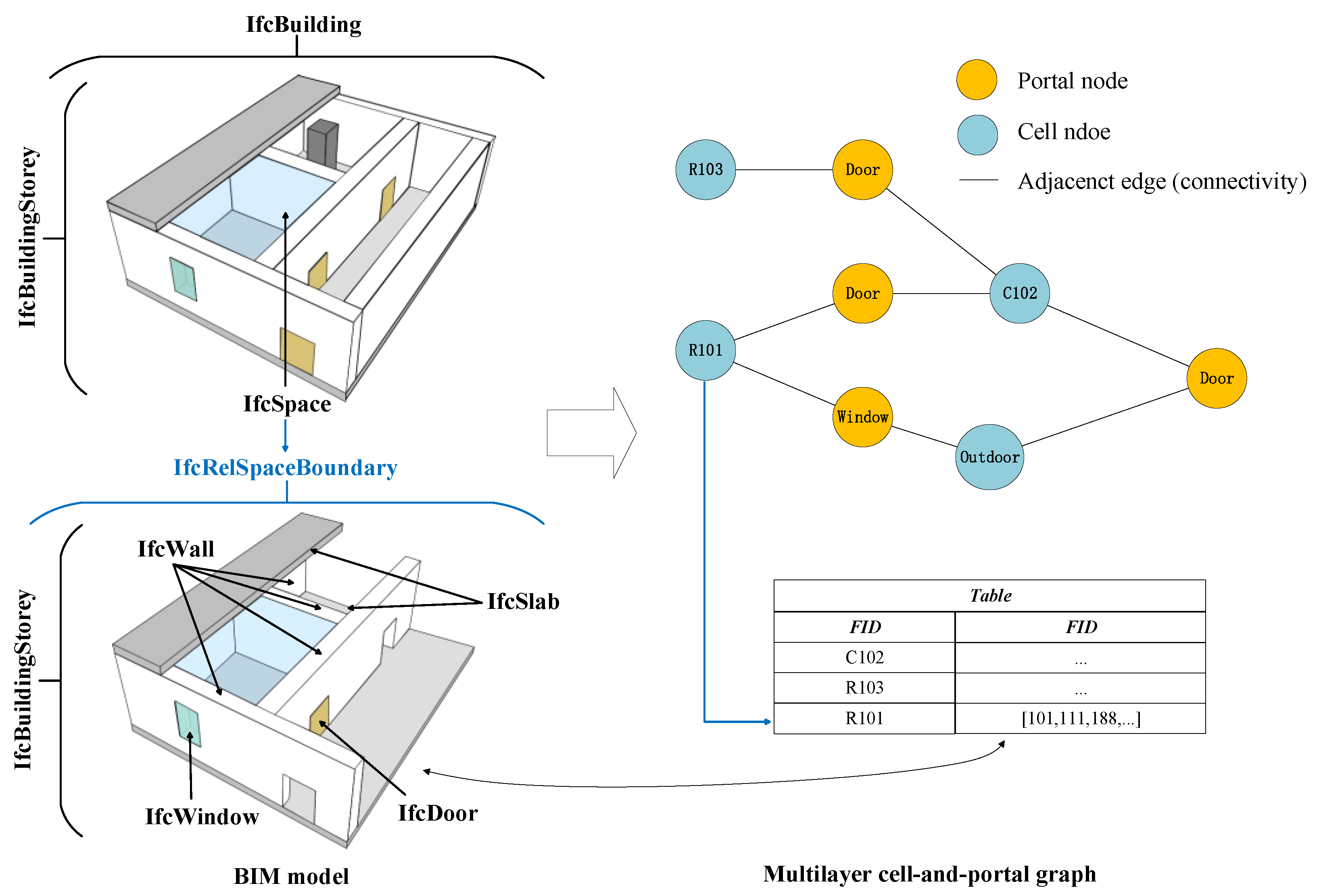
3.2.1. Semantic-Based Data Organization for Indoor Scenes in BIM Models

As shown in Figure 2, according to the IFC structure, we proposed a multilayer cell-and-portal graph for data index, represented by $G\left(V,E\right)$. The IfcSpace or outdoor space is abstracted as a node of the spatial structure $V_{cell}$. The node adds type, FID, and building entities associated with the associated space.

Portal entities (e.g., IfcWindow, IfcDoor, and IfcStair) define portal nodes ($V_{portal}$) in the graph (e.g., type, FID, and “visibility”, as described in Section 3.1). The edge in the graph represents the connection between nodes. Each building floor (IfcBuildingStorey) can create a single-layer cell-and-portal graph, and then floors are associated with each other through $V_{portal}\left(type=IfcStair\right)$, which finally forms the multilayer cell-and-portal graph in the BIM model.

The $V_{cell}\left(type=IfcSpace\right)$ can obtain related building entities based on semantics. For example, we can extract entities making up the room (or corridor) from the IfcRelSpaceBoundary in Figure 2. The related entities are stored in the $Table\left(FID,FIDs\right)$, where $FID$ denotes the unique identifier of IfcSpace, and $FIDs$ represent unique identifiers of building entities. Similarly, $V_{portal}$ stores two associated $V_{cell}$ in the $Table\left(FID,FID\right)$, where $FID$ indicates the unique identifier of IfcSpace. When $FID=-1$, $V_{cell}$ represents outdoor scenes.

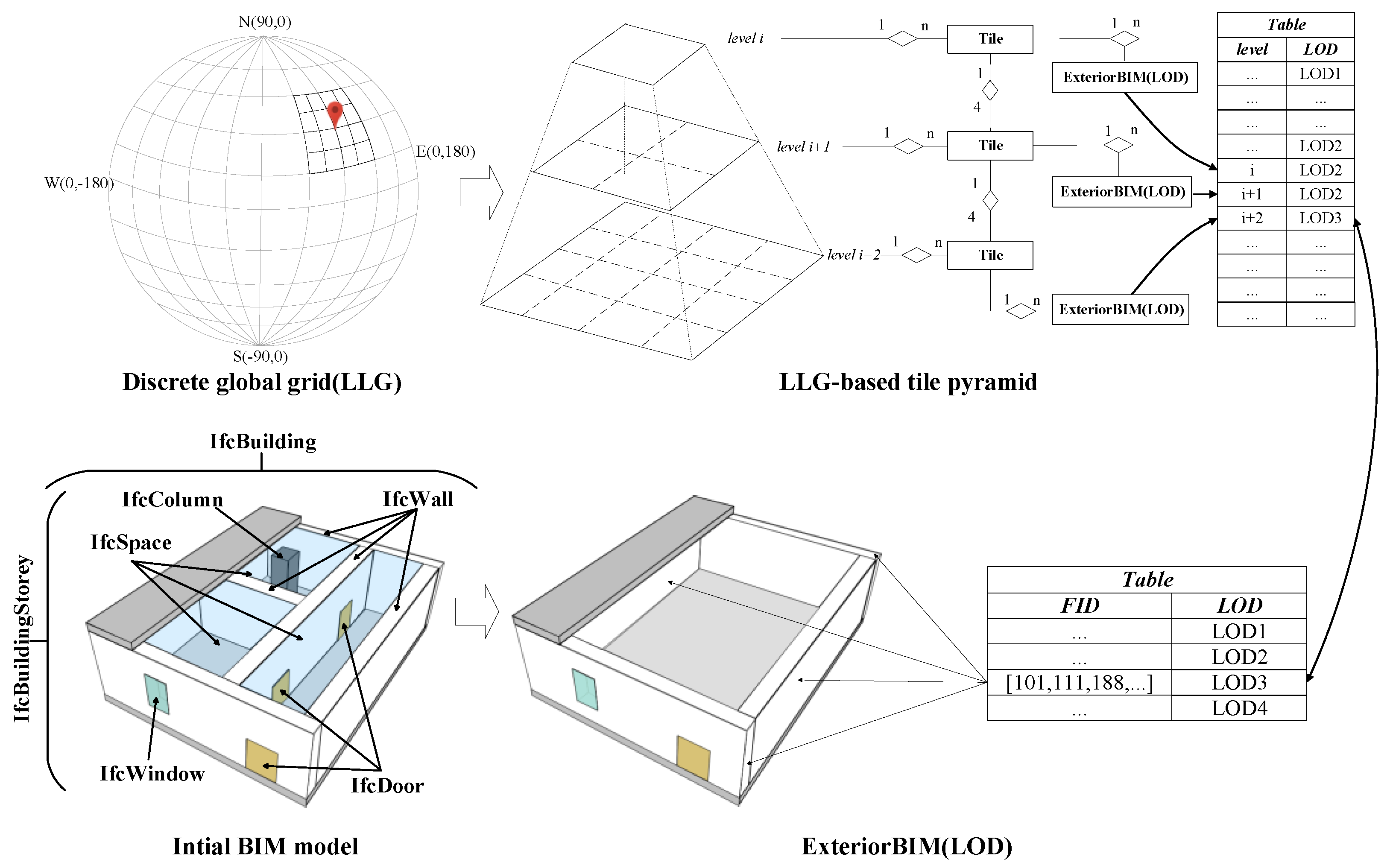
3.2.2. Semantic-Based Data Organization for Outdoor Scenes in BIM Models

As shown in Figure 3, exterior building entities ($ExteriorBIM$) first are obtained from each BIM model using previous algorithms that aim to reduce the computing burden [18,19]. Then, similar to other multi-scale GIS data sources (e.g., terrain, satellite imagery, and oblique aerial images) in virtual globes, we employ the LLG-based tile pyramid of the discrete global grid to organize the $ExteriorBIMs$ [12,34]. The $ExteriorBIM$ in the upper-level tile is simplified geometrically by the $ExteriorBIM$ in the lower-level tile. Explicitly, the multilayer cell-and-portal graph index building entities inside the $ExteriorBIM$ (Figure 2) and the portal node in the $ExteriorBIM$ have the following property: $FID=-1$ in two associated $V_{cell}$.

The geometric simplification means that the $ExteriorBIM$ is classified into different levels according to semantics, and each level contains entities of specified semantics. As shown in

Table 2. Hierarchical level of detail (LOD) for Building Information Modeling (BIM) models.

Level	IFC Type	Geometric Type
LOD1	IfcSite	Body
LOD2	IfcSlab, IfcRoof	Body
LOD3	IfcWall, IfcColumn	Body
LOD4	Other entities	Body

, we generated four LOD models from the $ExteriorBIM$ by IFC type. The continuous LOD strategy is inspired by Xu et al. (2020). For example, the LOD1 model only includes building entities named IfcSite. The LOD2 model consists of building entities named IfcSlab, IfcRoof, and IfcSite from the LOD1 model. Each LOD model includes an index table $Table\left(FIDs,LOD\right)$, in which $FIDs$ represents unique identifiers of building entities, LOD indicates the tile level, and $Table\left(FIDs,LOD\right)$ indexes the relationship between tiles and LOD. When LOD = 4, $ExteriorBIM\left(LOD\right)=ExteriorBIM$.

In particular, tiles and $ExteriorBIM\left(LOD\right)$ only are used as indices, and the geometry and semantics still are stored in the BIM model. The loading and rendering the BIM model depends on the distance from the viewpoint to the model center when browsing scenes.

3.3. Semantic-Based Scheduling Algorithm for Indoor/Outdoor Scenes in 3D GIS

According to the data organization in Section 3.2, we developed a semantic-based scheduling algorithm for indoor/outdoor scenes in 3D GIS (Algorithm 1). Algorithm 1 includes the following parts based on scene types: (1) semantic-based scheduling algorithm for indoor scenes in 3D GIS, (2) semantic-based scheduling algorithm for outdoor scenes in 3D GIS.

Since different method are used in different scene types, we first proposed a ray intersection algorithm to determine the current scene type. As shown in Figure 4, we constructed the central ray between the viewpoint and central point of the camera. The intersection result can identify the scene type. For example, when the ray intersects with the model and the first intersection is the IfcSpace, the scene type is indoors, otherwise it is outdoors. $ExteriorBIMs$ organized by an LLG-based tile pyramid can be quickly traversed to obtain visible data combined with view-frustum culling; this reduces the time needed to update the results [33].

Algorithm 1. Semantic-based scheduling algorithm for indoor scenes in 3D GIS
Input: Camera; Root node of LLG-based tile pyramid.
Output: BIM-GIS visualization.
1:	$\mathrm{Initialize}\mathrm{the}\mathrm{potential}\mathrm{visibility}\mathrm{set}:PVS=NULL$$;\mathrm{Set}type\left(environment\right)=outdoor$.
2:	$\mathrm{Calculate}\mathrm{the}\mathrm{current}\mathrm{extent}\mathit{Extent}({\mathit{lon}}_{\mathit{min}},{\mathit{lat}}_{\mathit{min}},{\mathit{lon}}_{\mathit{max}},{\mathit{lat}}_{\mathit{max}})$ from the camera.
3:	$\mathrm{Traverse}\mathrm{LLG}-\mathrm{based}\mathrm{tile}\mathrm{pyramid}\mathrm{according}\mathrm{to}\mathit{Extent}$$,\mathrm{and}\mathrm{thus}\mathrm{obtain}\mathrm{visible}\mathrm{tile}\mathrm{set}Tiles$.
4:	for$\mathrm{each}Tile$$\mathbf{in}Tiles$
5:	$\mathrm{Obtain}ExteriorBIMs$$\mathrm{from}Tile$.
6:	$\mathbf{for}\mathrm{each}ExteriorBIM$$\mathbf{in}ExteriorBIMs$
7:	$\mathbf{if}\mathrm{the}\mathrm{central}\mathrm{ray}\mathrm{from}\mathrm{camera}\mathrm{intersect}\mathrm{with}ExteriorBIM$ and the type of first intersection is IfcSpace
8:	$type\left(environment\right)=indoor$, go to Step2.
9:	end if
10:	end for
11:	end for
12:	if$type\left(environment\right)=indoor$
13:	$\mathrm{Step}1.\mathrm{semantic}-\mathrm{based}\mathrm{scheduling}\mathrm{algorithm}\mathrm{for}\mathrm{indoor}\mathrm{scenes}\mathrm{in}3\mathrm{D}\mathrm{GIS},\mathrm{return}\mathit{PVS}$.
14:	else
15:	$\mathrm{Step}2.\mathrm{semantic}-\mathrm{based}\mathrm{scheduling}\mathrm{algorithm}\mathrm{for}\mathrm{outdoor}\mathrm{scenes}\mathrm{in}3\mathrm{D}\mathrm{GIS},\mathrm{return}\mathit{PVS}$.
16:	end if
17:	$\mathrm{Send}PVS$ in the central processing unit (CPU) to the graphic processing unit (GPU) for model rendering.

3.3.1. Semantic-Based Scheduling Algorithm for Indoor Scenes in 3D GIS

For visualizing large-scale BIM models in indoor scenes, two issues must be addressed: (1) retaining only currently visible interior building entities from indoor views to reduce the computing burden; and (2) for the realistic visualization, the algorithm must identify the “visibility” to decide whether to load associated multi-scale GIS data, such as $ExteriorBIM\left(LOD\right)$ and oblique aerial images.

We proposed a semantic-based scheduling algorithm for indoor scenes in 3D GIS (Algorithm 2). This algorithm includes three key steps. First, building entities associated with the current IfcSpace are obtained according to the camera combined with the multilayer cell-and-portal graph (see Section 3.2.2); the entities are added to the $PVS$. Second, “visibility” is recognized by a similar method as described in Section 3.3.1, and used to determine whether the associated information is loaded. As shown in Figure 5, if “visibility” is false, the far plane of the camera is set as the diameter of the bounding sphere from the BIM model (Figure 5a); if “visibility” is true, the far plane is expanded, and associated entities and other multi-scale GIS data are added into the $PVS$ by view-frustum culling (Figure 5b). Finally, the $PVS$ is sent to the GPU for drawing.

Algorithm 2. Semantic-based scheduling algorithm for indoor scenes
Input: Camera; IfcSpace; $\mathit{threshold}=\mathrm{10,000}$.
Output:$\mathit{P}\mathit{V}\mathit{S}$.
1:	Set $PVS=NULL$ and $Distance=0$.
2:	Obtain building entities associated with IfcSpace and insert into $PVS$ by Section 3.2.2.
3:	Construct multiple rays parallel to the center ray in algorithm 1 around the view and obtain the intersection entity set $Set$.
4:	for each building entity in $Set$
5:	if “visibility” is true
6:	Obtain other $FID$ associated with the portal node by $Table\left(FID,FID\right)$.
7:	if $FID\ne -1$
8:	Obtain associated entities inside the BIM model, and add them into $PVS$ by $Table\left(FID,FIDs\right)$.
9:	$Distance=2\times radius$.
10:	else
11:	$Distance=threshold$.
12:	end if
13:	end if
14:	end for
15:	Set the distance of the far plane inside the camera is $Distance$, and add other $ExteriorBIMs$ into $PVS$ by view-frustum culling.
16:	return $PVS$.

3.3.2. Semantic-Based Scheduling Algorithm for Outdoor Scenes in 3D GIS

For visualizing large-scale BIM models on a virtual globe, a number of issues should be considered. First, efficient scheduling for BIM models combined with multi-scale GIS data (terrain, satellite imagery, and oblique aerial images) needs to be addressed. Second, the algorithm recognizes the semantic information from BIM/IFC, and then determines the “visibility” in the current view to realize a realistic visualization. For example, if there are transparent windows in the current scene, the associated entities in the indoor space should be loaded.

We proposed a semantic-based scheduling algorithm for outdoor scenes in 3D GIS, which is based on the scheduling algorithm in a virtual globe (Algorithm 3). First, visible $ExteriorBIM\left(LOD\right)s$ and multi-source GIS data can be filtered in the current view; they are then added into the potential visibility set ($PVS$). In particular, based on the LLG-based tile pyramid, the algorithm can quickly obtain the $PVS$ by view-frustum culling and can remove invisible data in time. Second, the algorithm identifies semantics (building type and property inside the BIM/IFC) to determine whether to load interior building entities. As shown in Figure 6, the algorithm generates multiple rays parallel to the central ray to intersect with $ExteriorBIM\left(LOD\right)$, and thus to acquire “visibility”. If “visibility” is true, the algorithm adds the interior entities to $PVS$ through the multilayer cell-and-portal graph (see Section 3.2.2). Finally, the $PVS$ is sent to the GPU for rendering.

Algorithm 3. Semantic-based scheduling algorithm for outdoor scenes
Input: Camera; Scene root.
Output: $\mathit{P}\mathit{V}\mathit{S}$.
1:	$\mathrm{Set}PVS=NULL$$\mathrm{and}\mathit{threshold}=15$.
2:	$\mathrm{Obtain}\mathrm{visible}ExteriorBIM\left(LOD\right)s$ and other GIS data sources by view-frustum culling.
3:	for$\mathrm{each}ExteriorBIM\left(LOD\right)$in$ExteriorBIM\left(LOD\right)s$.
4:	$\mathrm{Calculate}\mathrm{the}\mathrm{distance}\mathrm{from}\mathrm{the}\mathrm{viewpoint}\mathrm{to}\mathrm{the}ExteriorBIM\left(LOD\right)$ cener.   $\mathrm{Entities}\mathrm{of}\mathrm{LOD}\mathrm{models}\mathrm{are}\mathrm{added}\mathrm{to}PVS$$\mathrm{by}Table\left(FIDs,LOD\right)$$\mathrm{from}ExteriorBIM\left(LOD\right)$.
5:	end for
6:	$\mathrm{Construct}\mathrm{multiple}\mathrm{rays}\mathrm{parallel}\mathrm{to}\mathrm{the}\mathrm{center}\mathrm{ray}\mathrm{in}\mathrm{algorithm}1\mathrm{around}\mathrm{the}\mathrm{view}\mathrm{and}\mathrm{intersect}\mathrm{with}\mathrm{each}\mathrm{model}\mathrm{in}ExteriorBIM\left(LOD\right)$.
7:	if$\mathrm{rays}\mathrm{intersect}\mathrm{with}\mathrm{a}\mathrm{portal}\mathrm{node}\mathrm{and}\mathrm{the}\mathrm{intersected}\mathrm{distance}\mathrm{is}\mathrm{less}\mathrm{than}threshold$
8:	if “visibility” is true
9:	Obtain ID of the IfcSpace associated with the portal node.
10:	$\mathrm{Obtain}\mathrm{associated}\mathrm{entities}\mathrm{associated}\mathrm{with}\mathrm{the}\mathrm{IfcSpace},\mathrm{and}\mathrm{add}\mathrm{them}\mathrm{into}PVS$$\mathrm{according}\mathrm{to}Table\left(FID,FIDs\right)$.
11:	end if
12:	end if
13:	return$PVS$.

4. Results

4.1. Experimental Setup

To verify the validity of our proposed approach, the method was implemented in IfcPlusPlus for parsing IFC files and osgEarth, which is an open-source virtual globe. Experiments were conducted on a laptop with an Intel^® Core(TM)^® CPU i7-8750H @2.20GHz (Intel, Santa Clara, CA, USA), with one NVIDIA GeForce GTX1060 (NVIDIA, Santa Clara, CA, USA) and 8GB RAM (Samsung, Seongnam City, Gyeonggi Province, Korea).

As shown in Figure 7, different types of GIS data are available for the experimental region, located in China (labeled in yellow in Figure 7); these mainly include global satellite imagery from Google, oblique aerial images of ~2.51 GB in size, and BIM models. The $ExteriorBIM$ was extracted from the original IFC data, and divided into a four-level LOD hierarchy, in which the maximum visible distance is 1000 m. Building entities of the IfcSite were loaded when the distance was 1000 m(LOD1 model), and all building entities from $ExteriorBIM$ were loaded when the distance was 50 m(LOD4 model). Detailed geometric information for the experimental BIM model are given in

Table 3. Statistical results for the experimental model.

Type	No. of IfcProduct	No. of Vertices	No. of Triangles	Visible Distance (m)
Original BIM model	785	451,536	175,540	-
LOD1 model	1	1092	436	500~1000
LOD2 model	27	4356	1712	200~500
LOD3 model	75	107,456	40,567	50~200
$ExteriorBIM$ (LOD4 model)	282	209,800	80,508	<50

. Note, limited by the number of experiment data models, the experimental model was repeatedly loaded into the virtual globe 402 times to form large-scale BIM models in the virtual globe. The total data volume (of ~4.06 GB) included 180,614,400 vertices and 70,216,000 triangles.

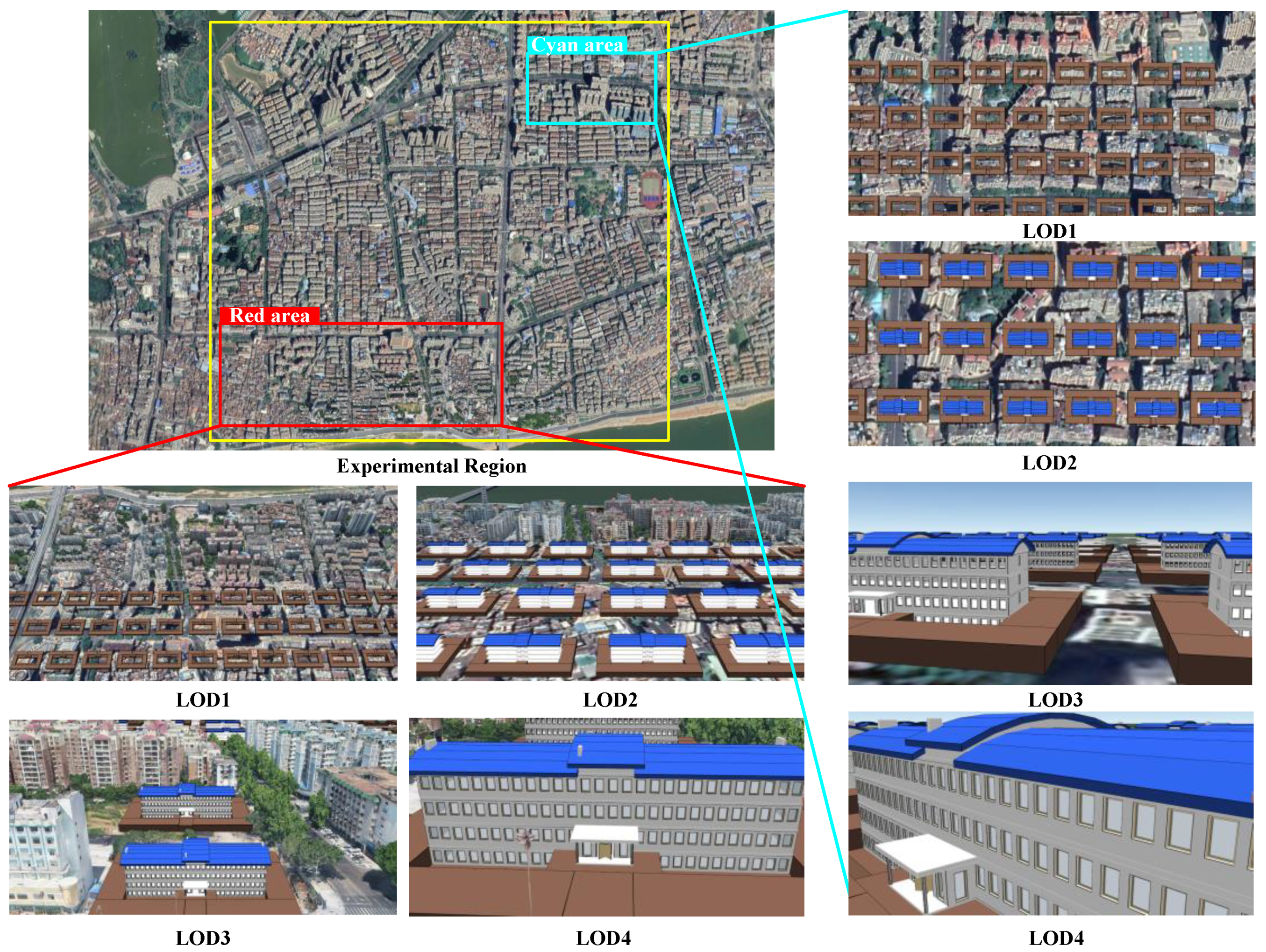
4.2. Validity Analysis of Large-Scale BIM Models in the Virtual Globe

To verify that our method can visualize huge BIM models in the virtual globe, the red area and cyan area in Figure 7 are selected to record the rendering efficiency of large-scale BIM models loaded at different distances. The average frames per second (FPS) at different distances can be found in Figure 8. Obviously, the average frame rate of both areas is higher than 60 FPS. Among them, the red area contains oblique aerial images and large-scale BIM models, and the average frame rate of this area is more than 83.60 FPS. Visual result about part results can be shown in Figure 8; The cyan area only contains BIM model data, and the average frame rate of this area is 78.28 FPS, and Figure 9 shows the part result; The cyan area only contains BIM model data, and the average frame rate of this area is 78.28 FPS, and visual results can be found in Figure 10. Therefore, the proposed method can maintain a higher frame rate from outdoor views when loading huge BIM models in the virtual globe, according to the above experiments.

4.3. Comparative Analysis of Experimental Results

Given that the method of Liu et al. (2016) optimizes the visualization of outdoor and indoor scenes, and also is a common strategy, we used it for the comparison with our proposed method. Note, we mainly simulated the indoor or outdoor visualization strategy for Liu’s method in the virtual globe.

4.3.1. Visualizing Outdoor Scenes

As shown in Figure 11, we selected two experimental areas with transparent windows for comparative analysis (labeled in green in Figure 11).

Using the Liu et al. (2016) method (Figure 12), when the viewpoint is located outdoors, interior building entities cannot be loaded when observing through a window. In contrast, using the proposed method, interior entities corresponding to the window are loaded when the viewpoint is close to the model and there is a transparent window (Figure 13).

When loading the interior entities inside the model at a close distance, our method inevitably increases the geometric data compared with the Liu et al. (2016) method. However, only entities associated with the portal are loaded, and the volume of increased geometry is limited (

Table 4. Statistical results for the experimental test.

Experimental Area	IfcProduct Number	No. of Vertices	No. of Triangles
Area 1	8	3418	1304
Area 2	11	3938	1507

).

As shown in Table 4, the numbers of incremental triangles relative to the original data for area 1 and area 2 were just 1.62% and 1.87%, respectively. For area 1, the average frames per second (FPS) before and after loading were 59.07 and 62.68 (Figure 14), respectively; for area 2, the average FPS before and after loading were 64.82 and 62.02 (Figure 15), respectively. The lack of significant change in FPS verifies the effectiveness of our proposed method.

4.3.2. Visualizing Indoor Scenes

The visualization of indoor GIS scenes mainly includes two cases: (1) the outdoor space is visible from the viewpoint and (2) the outdoor space is not visible from the viewpoint. These scenarios were compared using the Liu et al. (2016) method (Figure 16) and our proposed method (Figure 17).

When the outdoor scene is visible, the Liu et al. (2016) method results in an incomplete and unrealistic environment (Figure 16a), because it removes all outdoor models from indoor views, ignoring BIM/IFC semantics such as IfcWindow and transparency. In contrast, when the outdoor scene is not visible, interior entities are loaded completely (Figure 16b). In contrast, when using our proposed method, visible data (e.g., BIM models and oblique aerial images) were loaded and ensure a realistic environment when the view outdoors is visible (Figure 17a). When there is no view outdoors (Figure 17b), the visualization result is the same as those using the model of Liu et al. (2016).

Table 5. Statistical information for interior building entities when the outdoors is not visible.

Experimental Area	IfcProduct Number	No. of Vertices	No. of Triangles
Proposed method	50	30,360	11,577
Liu et al. (2016)	785	451,536	175,540

compares the statistical results for the different methods when the outdoor scene is not visible. The result proved that our method effectively reduced the geometric information: the building entities decreased by 735, and numbers of vertices and triangles were reduced by 421,176 and 163,963. In summary, our proposed method not only loads visible entities to indoor views, but also effectively reduces the computing burden by removing invisible indoor spaces in the building.

As shown in Figure 18, the average FPS over 1 min for the Liu et al. (2016) method and the proposed method were similar (~100 FPS).

Table 6. Statistical information for all building entities when the outdoors is visible.

Experimental Area	IfcProduct Number	No. of Vertices	No. of Triangles
Proposed method	332	240,160	92,085
Liu et al. (2016)	785	451,536	175,540

compares the statistical results for the different methods when the outdoor scene is visible. Using our proposed method, the building entities decreased by 453, the number of vertices decreased by 211,376, and number of triangles decreased by 83,455.

As shown in Figure 19, the average FPS over 1 min for the Liu et al. (2016) method higher than that of for our proposed method was (~100 FPS; lowest value = 98.64 FPS). These results confirm that our proposed method can more effectively ensure a realistic effect and simultaneously maintain a high frame rate.

5. Conclusions

For integrated visualization of BIM and 3D GIS, an outline culling algorithm can remove all occluded entities inside the BIM model from outdoor or indoor views; this reduces the geometric data volume while retaining the geometric accuracy and spatial characteristics of the BIM [18,19]. Nonetheless, previous studies have neglected special BIM semantics, and simply eliminated all building entities from indoor views or removed interior building entities from outdoor views, which resulted in a loss of geographic features and led to unreasonable visualization. Moreover, the methods explicitly did not focus on the visualization optimization in the indoor space, which may have required significant hardware resources for loading large and complex indoor buildings.

Therefore, we proposed a semantics-based method for visualizing large-scale BIM models within indoor and outdoor geographic environments. We analyzed the visualization and efficiency of our proposed method, and compared it with a previous method or strategy to verify the effectiveness of our approach:

(1)

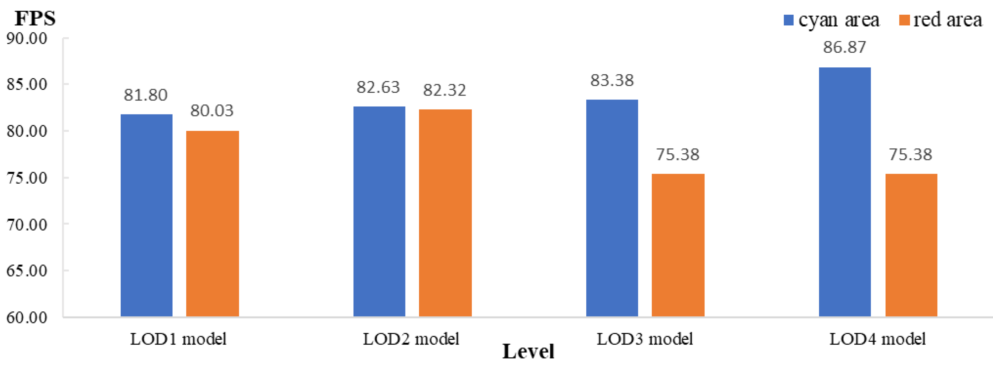
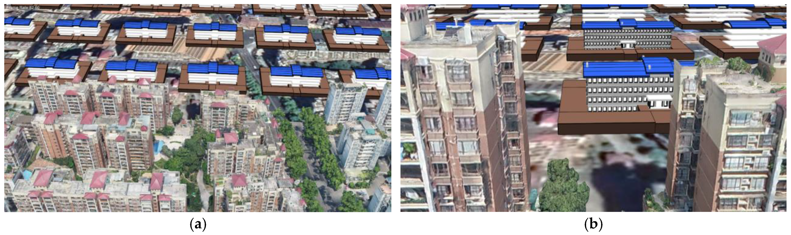
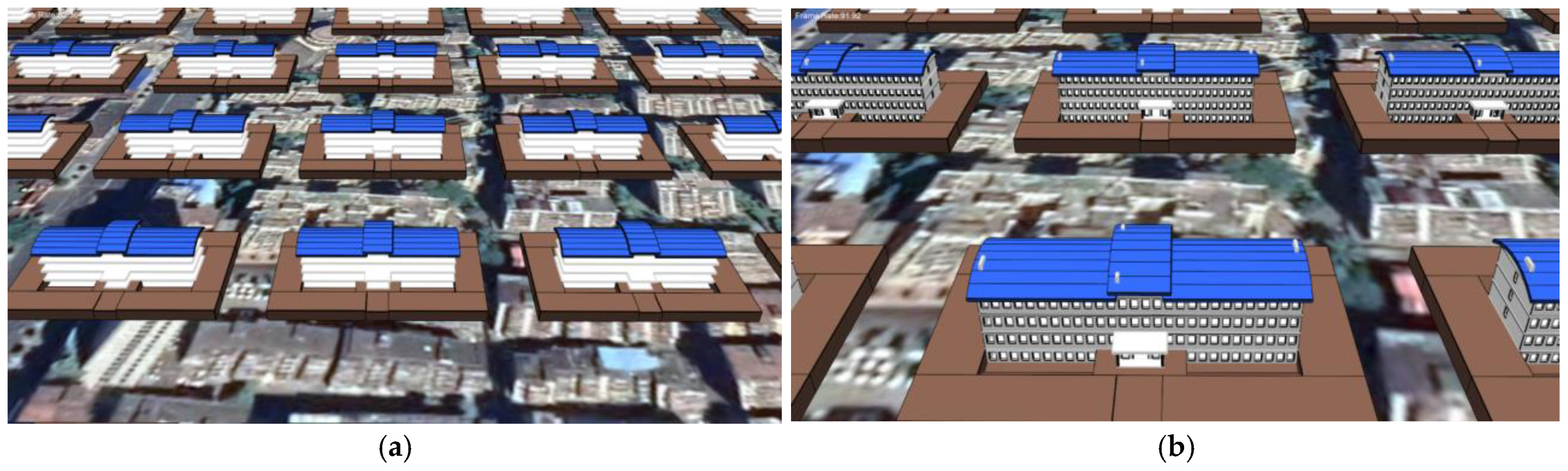
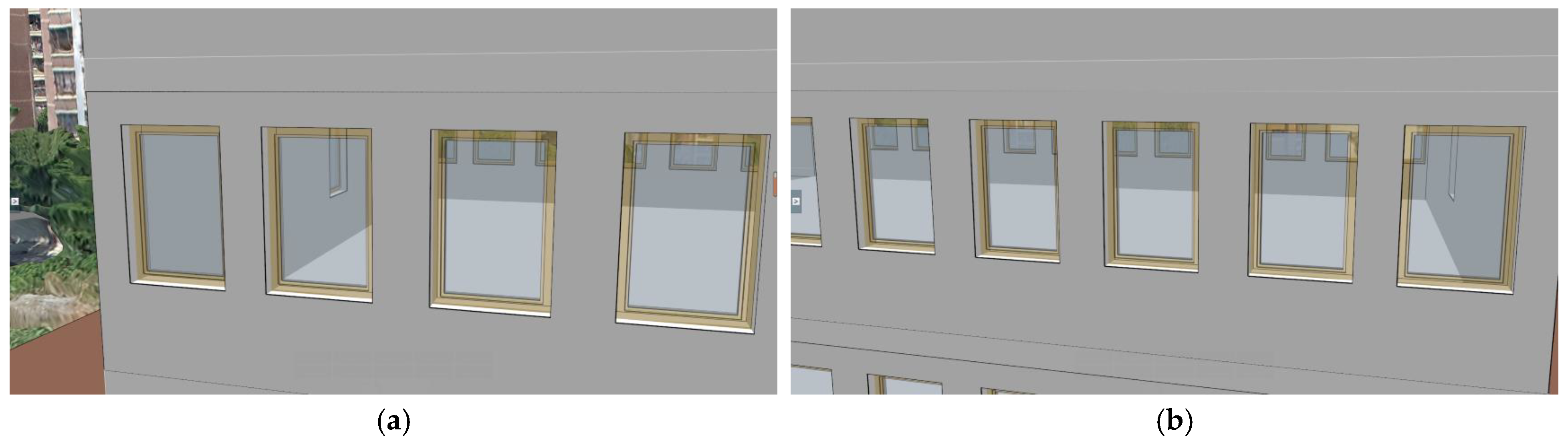
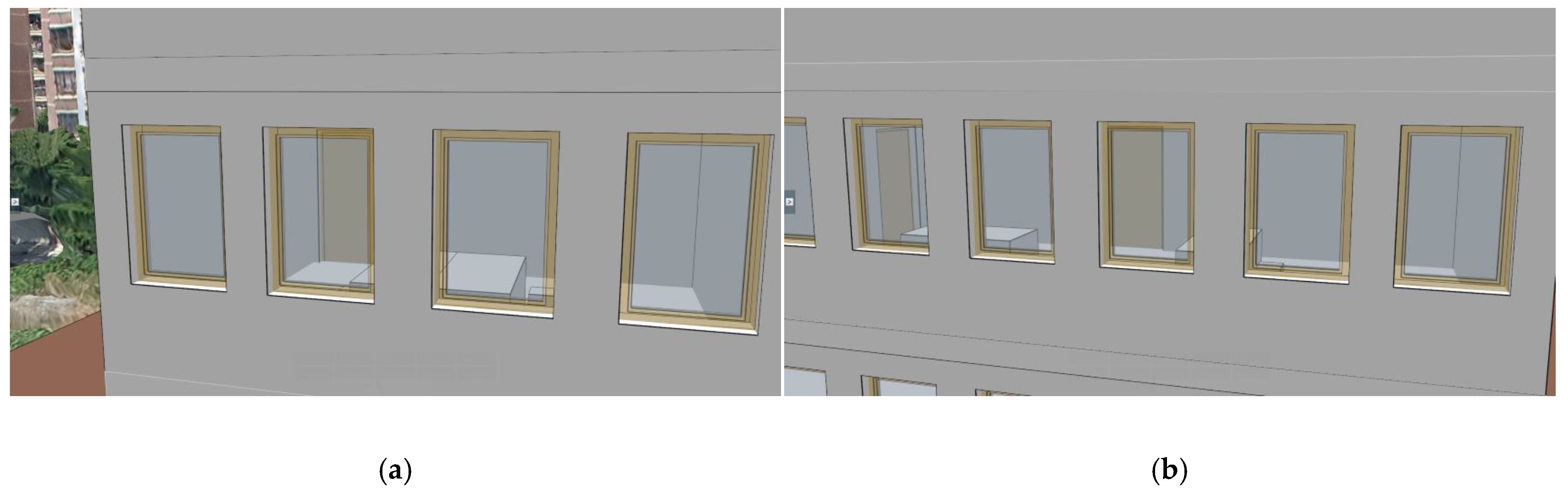
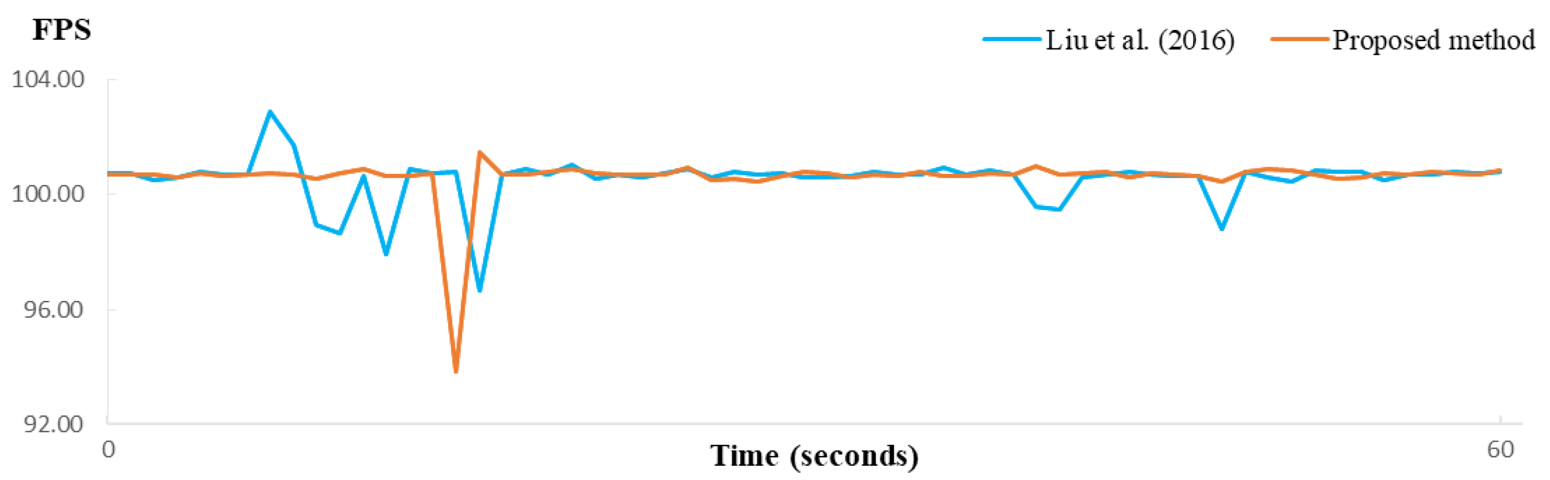
For outdoor scenes, the proposed LLG-based tile pyramid can effectively meet the visualization of large-scale BIM models on the virtual globe. When browsing windows and exterior entities, visible entities of the interior spaces viewed from outdoors are loaded, ensuring realistic visualization (Figure 12 and Figure 13) while effectively maintaining stable computing resources (Figure 14 and Figure 15).

(2)

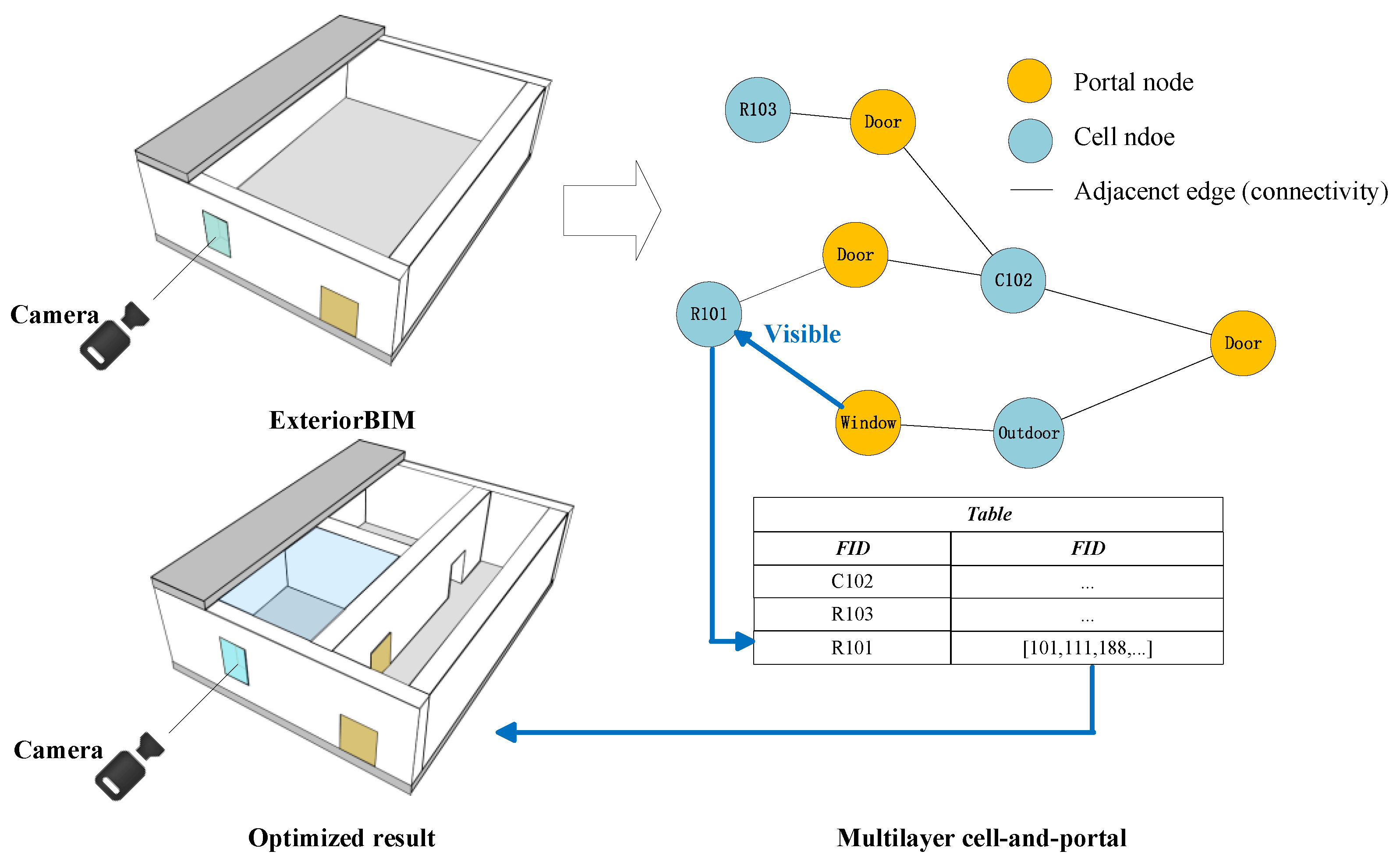
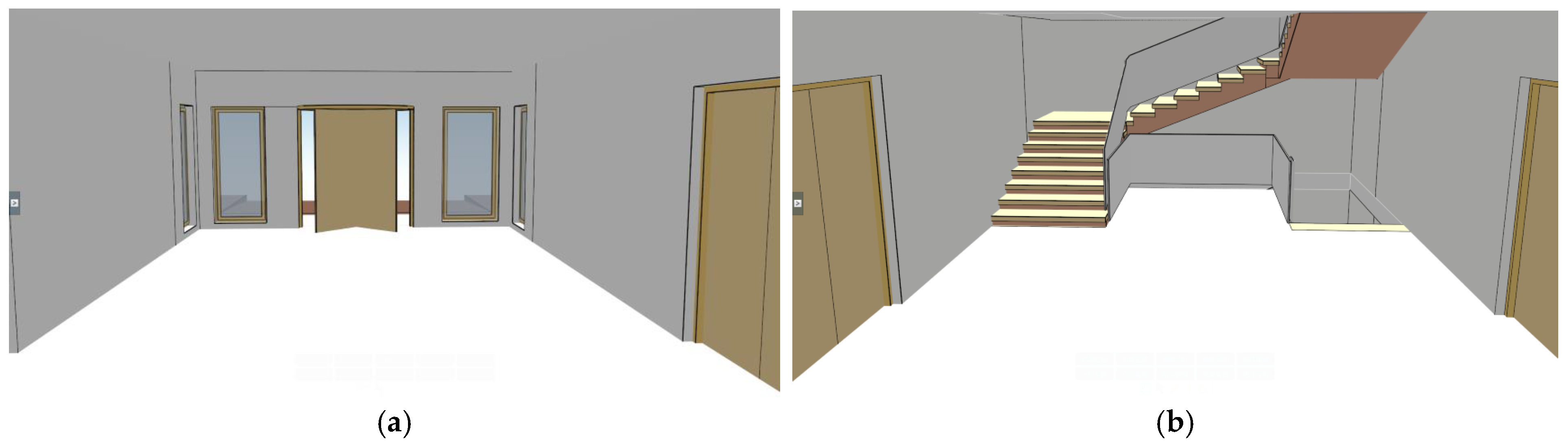
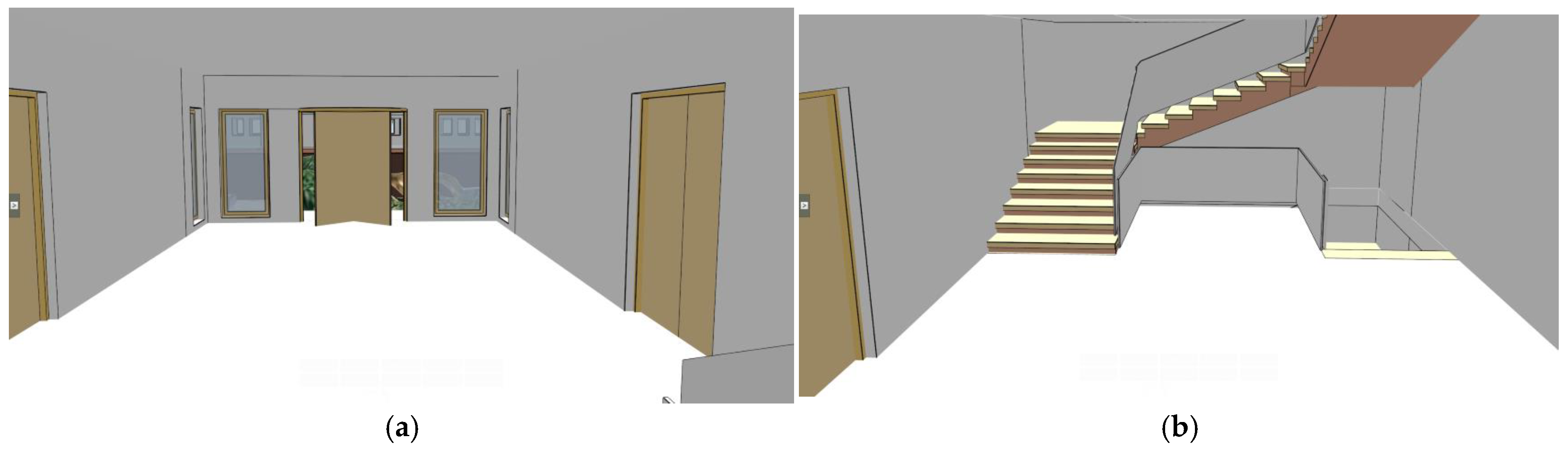
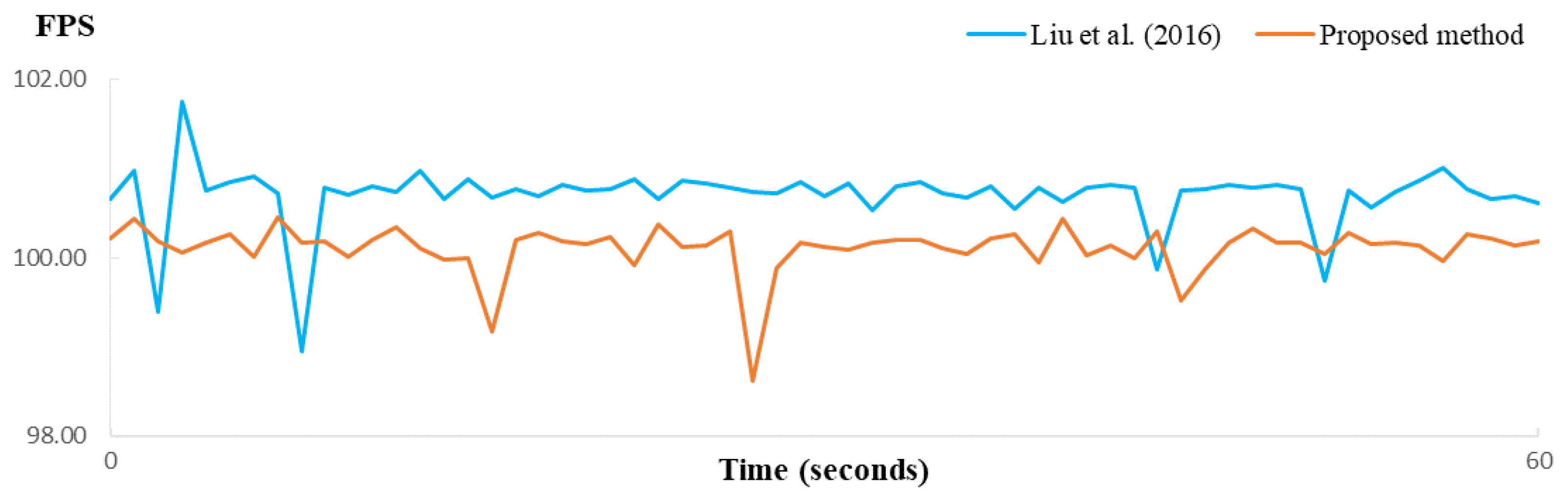
For indoor scenes, a multilayer cell-and-portal graph can effectively reduce the geometric data volume. For example, when browsing windows and interior entities, our method can unload other spaces (e.g., rooms) and load entities of current space according to the current location of the indoor space. Moreover, invisible BIM data from outdoor scenes is removed, which not only ensures realistic visualization (Figure 16 and Figure 17) but also effectively reduces the volume of geometric data (Figure 18 and Figure 19).

Our method can provide a solution for large-scale BIM models in the virtual globe. Besides, the study can observe indoor-outdoor environments from “visibility” components (such as a transparent window or open door) and retain a lower computing burden. Specifically, visible outdoor entities can be observed by the transparent window from indoor views, while other invisible entities are unloaded (or vice versa), which better facilitates the spatial analysis and application of the complex geometry and semantics of indoor and outdoor environments. For example, the study can support the roaming process from indoor to outdoor environments and solar radiation and lighting analyses in the green building [20], which avoid the shortcomings of previous studies.

However, our method still has some limitations. For example, we classify geographic scenes into two types (indoor and outdoor), and the proposed method cannot be directly applied to BIM models with no clear distinction between indoor and outdoor spaces. Besides, the indoor space of the building needs to be physically enclosed totally for indoor organization. Therefore, in the future, we will focus on a visualization method for the special BIM models mentioned above, such as special tree index, light-weighted technology, and other strategies. Moreover, achieving stable and efficient rendering of BIM models with different levels of hardware performance holds considerable promise.

References

1. Song, Y.; Wang, X.; Tan, Y.; Wu, P.; Sutrisna, M.; Cheng, J.; Hampson, K. Trends and Opportunities of BIM-GIS Integration in the Architecture, Engineering and Construction Industry: A Review from a Spatio-Temporal Statistical Perspective. ISPRS Int. J. Geo-Inf. 2017, 6, 397. [Google Scholar] [CrossRef] [Green Version]
2. Liu, X.; Wang, X.; Wright, G.; Cheng, J.; Li, X.; Liu, R. A State-of-the-Art Review on the Integration of Building Information Modeling (BIM) and Geographic Information System (GIS). ISPRS Int. J. Geo-Inf. 2017, 6, 53. [Google Scholar] [CrossRef] [Green Version]
3. IFC in ArcGIS—Bringing Open Standard BIM Data into GIS Workflows. Available online: https://technical.buildingsmart.org/idea/ifc-in-arcgis-bringing-open-standard-bim-data-into-gis-workflows/ (accessed on 3 November 2021).
4. Ivanov, R. An Approach for Developing Indoor Navigation Systems for Visually Impaired People Using Building Information Modeling. J. Ambient Intell. Smart Environ. 2017, 9, 449–467. [Google Scholar] [CrossRef]
5. Mahdaviparsa, A.; McCuen, T. Comparison between Current Methods of Indoor Network Analysis for Emergency Response Through BIM/CAD-GIS Integration. In Advances in Informatics and Computing in Civil and Construction Engineering; Mutis, I., Hartmann, T., Eds.; Springer International Publishing: Cham, Switzerland, 2019; pp. 627–635. ISBN 978-3-030-00219-0. [Google Scholar]
6. Teo, T.-A.; Cho, K.-H. BIM-Oriented Indoor Network Model for Indoor and Outdoor Combined Route Planning. Adv. Eng. Inform. 2016, 30, 268–282. [Google Scholar] [CrossRef]
7. Atazadeh, B.; Kalantari, M.; Rajabifard, A.; Ho, S.; Ngo, T. Building Information Modelling for High-Rise Land Administration. Trans. GIS 2017, 21, 91–113. [Google Scholar] [CrossRef]
8. Barzegar, M.; Rajabifard, A.; Kalantari, M.; Atazadeh, B. 3D BIM-Enabled Spatial Query for Retrieving Property Boundaries: A Case Study in Victoria, Australia. Int. J. Geogr. Inf. Sci. 2020, 34, 251–271. [Google Scholar] [CrossRef]
9. Shojaei, D.; Rajabifard, A.; Kalantari, M.; Bishop, I.D.; Aien, A. Design and Development of a Web-Based 3D Cadastral Visualisation Prototype. Int. J. Digit. Earth 2015, 8, 538–557. [Google Scholar] [CrossRef]
10. Amirebrahimi, S.; Rajabifard, A.; Mendis, P.; Ngo, T. A Framework for a Microscale Flood Damage Assessment and Visualization for a Building Using BIM–GIS Integration. Int. J. Digit. Earth 2016, 9, 363–386. [Google Scholar] [CrossRef]
11. Yamamura, S.; Fan, L.; Suzuki, Y. Assessment of Urban Energy Performance through Integration of BIM and GIS for Smart City Planning. Proc. Eng. 2017, 180, 1462–1472. [Google Scholar] [CrossRef]
12. Goodchild, M.F.; Guo, H.; Annoni, A.; Bian, L.; de Bie, K.; Campbell, F.; Craglia, M.; Ehlers, M.; van Genderen, J.; Jackson, D.; et al. Next-Generation Digital Earth. Proc. Natl. Acad. Sci. USA 2012, 109, 11088–11094. [Google Scholar] [CrossRef] [Green Version]
13. Yu, L.; Gong, P. Google Earth as a Virtual Globe Tool for Earth Science Applications at the Global Scale: Progress and Perspectives. Int. J. Remote Sens. 2012, 33, 3966–3986. [Google Scholar] [CrossRef]
14. Xu, Z.; Zhang, L.; Li, H.; Lin, Y.-H.; Yin, S. Combining IFC and 3D Tiles to Create 3D Visualization for Building Information Modeling. Autom. Constr. 2020, 109, 102995. [Google Scholar] [CrossRef]
15. Zhan, W.; Chen, Y.; Chen, J. 3D Tiles-Based High-Efficiency Visualization Method for Complex BIM Models on the Web. ISPRS Int. J. Geo-Inf. 2021, 10, 476. [Google Scholar] [CrossRef]
16. Tolmer, C.-E.; Castaing, C.; Diab, Y.; Morand, D. CityGML and IFC: Going Further than LOD. In Proceedings of the 2013 Digital Heritage International Congress (DigitalHeritage), Marseille, France, 28 October–1 November 2013; pp. 645–648. [Google Scholar]
17. Kim, J.-S.; Li, K.-J. Simplification of Geometric Objects in an Indoor Space. ISPRS J. Photogramm. Remote Sens. 2019, 147, 146–162. [Google Scholar] [CrossRef]
18. Zhou, X.; Zhao, J.; Wang, J.; Su, D.; Zhang, H.; Guo, M.; Guo, M.; Li, Z. OutDet: An Algorithm for Extracting the Outer Surfaces of Building Information Models for Integration with Geographic Information Systems. Int. J. Geogr. Inf. Sci. 2019, 33, 1444–1470. [Google Scholar] [CrossRef]
19. Liu, X.; Xie, N.; Tang, K.; Jia, J. Lightweighting for Web3D Visualization of Large-Scale BIM Scenes in Real-Time. Graph. Models 2016, 88, 40–56. [Google Scholar] [CrossRef]
20. Lu, Y.; Wu, Z.; Chang, R.; Li, Y. Building Information Modeling (BIM) for Green Buildings: A Critical Review and Future Directions. Autom. Constr. 2017, 83, 134–148. [Google Scholar] [CrossRef]
21. Peterson, P.R. Discrete Global Grid Systems. In International Encyclopedia of Geography: People, the Earth, Environment and Technology; Richardson, D., Castree, N., Goodchild, M.F., Kobayashi, A., Liu, W., Marston, R.A., Eds.; John Wiley & Sons, Ltd.: Oxford, UK, 2017; pp. 1–10. ISBN 978-0-470-65963-2. [Google Scholar]
22. de Laat, R.; van Berlo, L. Integration of BIM and GIS: The Development of the CityGML GeoBIM Extension. In Advances in 3D Geo-Information Sciences; Kolbe, T.H., König, G., Nagel, C., Eds.; Springer: Berlin/Heidelberg, Germany, 2011; pp. 211–225. ISBN 978-3-642-12669-7. [Google Scholar]
23. Donkers, S.; Ledoux, H.; Zhao, J.; Stoter, J. Automatic Conversion of IFC Datasets to Geometrically and Semantically Correct CityGML LOD3 Buildings: Automatic Conversion of IFC Datasets to CityGML LOD3 Buildings. Trans. GIS 2016, 20, 547–569. [Google Scholar] [CrossRef] [Green Version]
24. Deng, Y.; Cheng, J.C.P.; Anumba, C. Mapping between BIM and 3D GIS in Different Levels of Detail Using Schema Mediation and Instance Comparison. Autom. Constr. 2016, 67, 1–21. [Google Scholar] [CrossRef]
25. Chen, Y.; Shooraj, E.; Rajabifard, A.; Sabri, S. From IFC to 3D Tiles: An Integrated Open-Source Solution for Visualising BIMs on Cesium. ISPRS Int. J. Geo-Inf. 2018, 7, 393. [Google Scholar] [CrossRef] [Green Version]
26. Varduhn, V.; Mundani, R.P.; Rank, E. Real Time Processing of Large Data Sets from Built Infrastructure. J. Syst. Cybern. Inform. 2011, 9, 63–67. [Google Scholar]
27. Borrmann, A.; König, M.; Koch, C.; Beetz, J. (Eds.) Building Information Modeling: Technology Foundations and Industry Practice; Springer International Publishing: Cham, Switzerland, 2018; ISBN 978-3-319-92861-6. [Google Scholar]
28. Liebich, T. IFC4—The New BuildingSMART Standard; AEC3 Ltd.: High Wycombe, UK, 2013. [Google Scholar]
29. Uggla, G.; Horemuz, M. Geographic Capabilities and Limitations of Industry Foundation Classes. Autom. Constr. 2018, 96, 554–566. [Google Scholar] [CrossRef]
30. Arroyo Ohori, K.; Diakité, A.; Krijnen, T.; Ledoux, H.; Stoter, J. Processing BIM and GIS Models in Practice: Experiences and Recommendations from a GeoBIM Project in The Netherlands. ISPRS Int. J. Geo-Inf. 2018, 7, 311. [Google Scholar] [CrossRef] [Green Version]
31. Chen, Q.; Chen, J.; Huang, W. Method for Generation of Indoor GIS Models Based on BIM Models to Support Adjacent Analysis of Indoor Spaces. ISPRS Int. J. Geo-Inf. 2020, 9, 508. [Google Scholar] [CrossRef]
32. Diakite, A.A.; Zlatanova, S. Automatic Geo-Referencing of BIM in GIS Environments Using Building Footprints. Comput. Environ. Urban Syst. 2020, 80, 101453. [Google Scholar] [CrossRef]
33. Cohen-Or, D.; Chrysanthou, Y.L.; Silva, C.T.; Durand, F. A Survey of Visibility for Walkthrough Applications. IEEE Trans. Vis. Comput. Graph. 2003, 9, 412–431. [Google Scholar] [CrossRef] [Green Version]
34. Dong, Q.; Chen, J. A Tile-Based Method for Geodesic Buffer Generation in a Virtual Globe. Int. J. Geogr. Inf. Sci. 2018, 32, 302–323. [Google Scholar] [CrossRef]
Figure 1. Building information modeling (BIM)/Industry Foundation Classes (IFC) data organization.
Ijgi 10 00756 g001
Figure 2. Multilayer cell-and portal graph.
Ijgi 10 00756 g002
Figure 3. Data organization for large-scale Building Information Modeling (BIM) models in outdoor scenes.
Ijgi 10 00756 g003
Figure 4. Intersection of the center ray and building. (a) Outdoor and (b) indoor scenes.
Ijgi 10 00756 g004
Figure 5. Semantic-based scheduling algorithm for outdoor scenes. Scheme to (a) remove outdoor Building Information Modeling (BIM) models and (b) load outdoor BIM models.
Ijgi 10 00756 g005
Figure 6. Ray intersection for outdoor scenes.
Ijgi 10 00756 g006
Figure 7. Oblique view of the experimental region from different distance.
Ijgi 10 00756 g007
Figure 8. Average frames per second (FPS) for cyan area and red area.
Ijgi 10 00756 g008
Figure 9. BIM models and oblique aerial images for the red area: (a) LOD2 (level-of-detail) models; (b) LOD3 models.
Ijgi 10 00756 g009
Figure 10. BIM models for the cyan area: (a) LOD2 models; (b) LOD3 models.
Ijgi 10 00756 g010
Figure 11. Experimental areas (within green dashed lines) for testing outdoor scenes.
Ijgi 10 00756 g011
Figure 12. Results of the Liu et al. (2016) method. (a) Area 1 and (b) area 2 of Figure 11.
Ijgi 10 00756 g012
Figure 13. Results of the proposed method. (a) Area 1 and (b) area 2 of Figure 11.
Ijgi 10 00756 g013
Figure 14. Average frames per second (FPS) before and after loading for experimental area 1.
Ijgi 10 00756 g014
Figure 15. Average frames per second (FPS) before and after loading for experimental area 2.
Ijgi 10 00756 g015
Figure 16. Model output based on the Liu et al. (2016) strategy. (a) Visible and (b) invisible outdoor scenes.
Ijgi 10 00756 g016
Figure 17. Model output based on the proposed method. (a) Visible and (b) invisible outdoor scenes.
Ijgi 10 00756 g017
Figure 18. Average frames per second (FPS) for indoor scenes inside the Building Information Model (BIM) model when the outdoors is not visible.
Ijgi 10 00756 g018
Figure 19. Average frames per second (FPS) for indoor scenes inside the Building Information Model (BIM) model when the outdoors is visible.
Ijgi 10 00756 g019