Geospatial and Machine Learning Regression Techniques for Analyzing Food Access Impact on Health Issues in Sustainable Communities

Abstract

Food access is a major key component in food security, as it is every individual’s right to proper access to a nutritious and affordable food supply. Low access to healthy food sources influences people’s diet and activity habits. Guilford County in North Carolina has a high ranking in low food security and a high rate of health issues such as high blood pressure, high cholesterol, and obesity. Therefore, the primary objective of this study was to investigate the geospatial correlation between health issues and food access areas. The secondary objective was to quantitatively compare food access areas and heath issues’ descriptive statistics. The tertiary objective was to compare several machine learning techniques and find the best model that fit health issues against various food access variables with the highest performance accuracy. In this study, we adopted a food-access perspective to show that communities that have residents who have equitable access to healthy food options are typically less vulnerable to health-related disasters. We propose a methodology to help policymakers lower the number of health issues in Guilford County by analyzing such issues via correlation with respect to food access. Specifically, we conducted a geographic information system mapping methodology to examine how access to healthy food options influenced health and mortality outcomes in one of the largest counties in the state of North Carolina. We created geospatial maps representing food deserts—areas with scarce access to nutritious food; food swamps—areas with more availability of unhealthy food options compared to healthy food options; and food oases—areas with a relatively higher availability of healthy food options than unhealthy options. Our results presented a positive correlation coefficient of R² = 0.819 among obesity and the independent variables of transportation access, and population. The correlation coefficient matrix analysis helped to identify a strong negative correlation between obesity and median income. Overall, this study offers valuable insights that can help health authorities develop preemptive preparedness for healthcare disasters.

1. Introduction

City planning for sustainable communities requires equitable distribution of and access to healthy food options for inhabitants. This study examined the statistical association between food access on people’s health and its connection to income and mobility access. The unbalanced distribution of food may have consequences concerning health and other factors. In this study, we examined these issues in Guilford County, North Carolina. Guilford County was ranked as the highest in food scarcity in North Carolina by the Food Research and Action Center in 2020 [1]. Since then, the county has worked to analyze the factors associated with food scarcity, studying the area’s income, education, and poverty rates. To advance Guilford County from a scarcity condition to sustainable equal distribution condition, an estimate of the scarcity situation and an analysis of the geographic areas for improvements in food access were needed. A key objective of sustainable communities is to effectively manage the health issues of their inhabitants. The process included gauging food access distribution by spatial methods, analyzing potential factors, and finding areas with remarkable numbers to start development. Recent studies have examined the distribution of food outlets and peoples’ buying habits and their food options. However, there are several studies that have presented the investigation of food outlets’ distribution geographically by integrating the health issues correlations to people’s habits or food distribution. This study focused on the density of food outlets, the health issues regarding the food outlets’ distribution, food access areas, and its correlation in terms of income, vehicle access, and health issues. Ultimately, we also simulated an improvement to provide suggestions and strategies for enabling Guilford County to become a smart, sustainable community in terms of food access.

Planning future cities requires scientists’ and planners’ points of views in solving current issues and prioritizing the service sectors according to the areas’ needs. As a result, concepts, such as smart cities, intelligent cities, sustainable cities, and creative cities, were invented. The definitions of these concepts vary from one author to another based on the planning priorities. Several models have been applied to investigate health-related issues. A socio-ecological model (SEM) is an approach that investigates health as influenced by environment, social, policy, and physical factors [2]. SEM investigates levels of influence at the interpersonal, institutional, community, and public policy levels [2]. This model investigated factors at each layer to understand their relationships [3]. Nevertheless, this model estimated prediction [4]. For instance, a study presented the application of the SEM model to investigate obesity-related variables such as vesical activities [3]. The layers that presented the strongest on predicting childhood obesity were neighborhood characteristics, parent demographics, and parent participation in their community [3].

According to [5], more advanced management technology can be used to manage a city’s resources and provide security [5]. In city planning, food access is primarily analyzed by scientists and decision makers to show its influence on the health of people living in these areas [6]. Food security and access were measured using several methods. Several techniques and methods were applied to measure food distribution and security. Measuring the geographical location of food outlets was performed based on applying GIS methods and tools. GIS is a software manager that analyzes data based on their geographical location [7]. GIS is applied to a wide range of problems such as natural hazards and public health [8]. GIS methods were used in different food analyses such as buffering, kernel density estimation, and spatial clustering [7]. More methods were applied depending on surveys and statistical data. For instance, an example method was based on the retail food environment index (RFEI) [9]. However, some methods have limitations concerning the application and presentation of results. The RFEI method has the limitation of not covering all tracts because of the need of calculating all food outlets categories such as supermarkets [9]. A study performed in California showed that data maples covered only 3719 out of 7049 based on the RFEI method [9].

Techniques, such as machine learning, are now used for research related to food security, as they are highly data-driven models. Machine learning (ML) is a programming technique that is used to solve nonlinear problems efficiently. It has models and algorithms, where the algorithm executes on the data to create the model [10]. It has serval different models to investigate relationships and compare results. The ML techniques were used to solve major problems such as classification, regression, reinforcement, and clustering [11]. The regression analysis was applied to detect continuous metric output [12]. Regression problems were investigated by several models, for instance, linear and nonlinear regression. These models also worked in hyper feature space for illustrating the relationship and were applied to different scientific fields [13]. A further example is the K-nearest neighbors regression model, which presents appealing results for small data [14]. Random forest regression models, as part of tree multioutput regression, were used to predict the variables [12]. More than one regression analysis can be used in comparison to find the best-suited model for higher performance. A study investigated food security using machine learning models (extreme gradient boosting, random forest, and CatBoost) to predict monthly variations [15]. This study investigated data involving food choices, income, geographical location, and climate [15]. It showed Xgboost was the best model and better results were presented when fewer changes in time and place accrued [15]. A further study in food security discussed the application of machine learning techniques to predict the modified retail food environment index (mRFEI) and found that a food desert differs from a food swamp thereby necessitating the application of different policies [16].

Furthermore, sustainable communities give priority to people’s health [5]. However, currently, it is recommended to use smart and sustainable terms as one concept, which converges the application of data-driven technologies of smart cities with the key goal of creating sustainable communities to provide an equal right to the benefits and an equal access to healthy food [17].

Studying the distribution of food outlets involves studying the distribution of groceries, restaurants, and residents’ density. Food access can be analyzed by studying the two key elements known as a food desert and a food swamp. Food swamps are areas with more unhealthy food options than healthy food options [18]. On the other hand, food deserts represent areas with low access to healthy food, and the expected distance was 500 meters, 0.3 miles, or 5–7 minutes of walking [19]. The characteristics of food deserts include availability of inexpensive food, poor nutrition, and limited healthy items in small stores [18]. Food insecurity is not only the critical area to be investigated. The availability of food sources is also very important. Food oases represent areas where people have an abundance of healthy food options rather than unhealthy food options [20]. In another study, the difference between food item prices was investigated with respect to food access areas, food deserts, food swamps, and food oases, and it was determined that there were no remarkable differences in the process [20].

Several studies investigated the influence between food distribution and other variables such as location, transportation, time, and behavior. A study of 36 counties of a suburban area showed that these areas suffered because residents needed to travel up to 30 miles for healthy food access [21]. Another study analyzed food access in the suburban areas and rural areas of Louisiana and determined that suburban areas near urbanization had greater access to healthy food [22]. Time could be analyzed by two dimensions including the time of events (such as weather events) and the time of source existence (such as food trucks and farmers’ markets) [6]. For example, the accessibility of food by walking was found to be different in summer than in winter, as the time of the year and day were different. As a result, in the case of a health disaster, socially isolated communities with food scarcity were most severely affected [23]. A study applied GIS and analyzed people’s access to transportation where the results indicated the importance of transportation access to improve people’s food choices [24]. Another study analyzed people’s behavior using data from an application designed for people to donate food [25]. The results showed a correlation between a higher number of donations points and more bus stops as a means of access to transportation [25].

Analyzing food access is a complex process that includes observing the current distribution of food outlets and analyzing the residents using different methods, factors, and scenarios. These factors were transportation access to supermarkets, the ethnic group of population distribution in food deserts, economic status, and chain and non-chain stores [26]. A study by Eckert and Shetty (2011) used block methods in geographic information systems (GIS), which applied network analysis to determine the distance between each resident and the grocery store (considering the residents’ ethnic group and income) [27]. The result showed that there was no connection between income and ethnic group in relation to food access [27]. Regarding chain and non-chain stores, a report by the Economic Research Service (ERS) explained that smaller stores sold smaller packages at a higher cost compared to supermarkets and non-chain stores [26]. Moreover, they were typically situated in poorer areas [26]. Another study showed that more options for greater food items were available with lower prices in supermarkets compared to small stores [28].

One study on food access and its consequences examined the relationship between fast-food restaurants and obesity in the surrounding areas [29]. The study considered two miles as the accessibility distance to analyze the health records but found no connection between obesity and fast-food accessibility [29]. Another study in Philadelphia, which was considered the second lowest in food access among major cities nationally, concluded that many low-income and food access neighborhoods had a high number of health challenges such as diabetes, heart diseases, and cancer [26]. An additional study also found a connection between food deserts, low income, lack of transportation, and diabetes [30].

There have been several studies on the consequences of inadequate food distribution, and they included the number of diseases spreading. Healthy food access was a key factor in the obesity epidemic, and the high consumption of unhealthy food was a critical factor in diabetes, hypertension, cancer, high mortality rates, and life loss [18]. There were some studies on the health risks and mortality rates regarding food access, and some of these suggested looking into the factors of these rates after mapping them. A study by Cossman and others (2003) mapped the mortality rates in every county in the United States for 30 years and determined the highest and lowest mortality rates [31]. The study suggested looking into the continuous high mortality in a county and analyzing it to determine the involved factors [31]. Another study looked into mapping health issues, such as tuberculosis, and the correlation with human development such as food access, income, education, and health [32]. The study concluded that there was a connection between human development and tuberculosis [32], where neighborhoods with less than the average income and education had higher tuberculosis rates [32]. A further study illustrated the investigation of type 2 diabetes per county level by machine learning [33]. Its results illustrated no correlation between the health issue and the variables of physical activities, access to exercise, and food environment [33].

Several limitations on food access were presented in recent studies. A large percentage of studies focused on only one to two outlets or categories, and only a few investigated the effect of all types of food outlets [34]. Another method’s limitation involved hypothesizing that people’s health was only influenced by the stores located closed to their residential location [34]. A further limitation involved using separate methods concerning food, where nutrition studies were separated from food environment research (combining them with the support of more methods and techniques would present a comprehensive overview of food access and health consequences) [34].

The reviewed literature illustrated that several studies focused on a few parts or variables of the overall problem regarding food access, health issues, and regional distribution. We studied all food access areas together with their influence on three health issues as a holistic case and to help local authorities in decision making for future planning. According to the literature review, food scarcity was studied in the form of a food desert and food swamp but lacked their influence on health conditions and the comparison to food abundance. The research questions in this study were:

Using GIS spatial mapping, can we find possible correlations between food access distribution and health risk issues?

Do health issues depend solely on univariate food access distribution or multivariate analysis of transportation access, income, population, and food access?

Can the linear or nonlinear ML regression models be developed for dependent variable health risks with better determinant coefficient?

This study addressed the gap by finding the correlations of food desert factors, food swamps, and food oases impacting on health issues and mortality using geospatial in-formation analysis, surveys, and machine learning techniques. Our contributions in this study included reporting the results of:

Investigating the geospatial correlation between food distribution and health issues;

Comparing the number of health issues between food access areas;

Estimating the statistical correlation between health issues and several variables;

Comparing the results of the regression analysis models regarding health issues related to several variables.

2. Materials and Methods

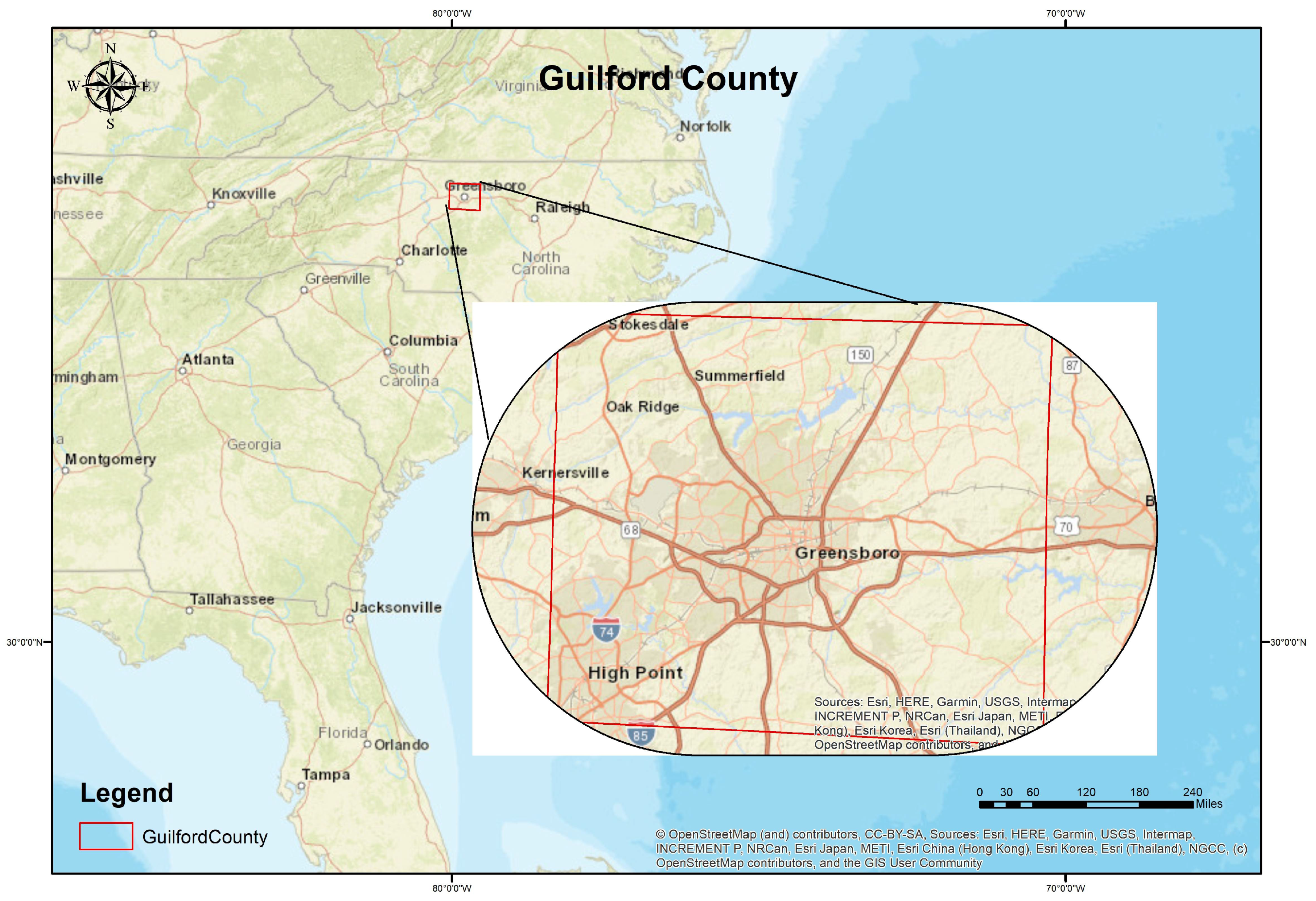
We examined Guilford County in North Carolina as our study area (Figure 1) including tabular attribute data. Data were obtained from the Health Department in Greensboro based on a crude survey, USDA Environmental Atlas, and the American Community Survey. Health records were collected by the North Carolina Department of Public Health. These data were geolocated by tracts. The data included income, food outlets, health records, low transportation aces, and mortality rates. Health records included (i) high cholesterol, where cholesterol was higher than 240 mg/dL and higher than 18% lipoprotein density; (ii) high blood pressure, where the systolic was 140 mm and diastolic was 90 mm or higher; (iii) obesity as defined by the World Health Organization, when an individual’s body mass was greater than 30 [35,36,37]. At the time of this study, Guilford County aimed to become a smart, sustainable community. With a population of 533,670 within 645.70 square miles, it was the third most populated county in North Carolina and was also among the top five most densely populated counties in the state of North Carolina [20]. It was also the largest county in terms of acreage [38,39]. Guilford County had 118 census tracts, and it covered the cities of Greensboro and Highpoint and eight towns consisting of Gibsonville, Jamestown, Oak Ridge, Pleasant Garden, Sedalia, Stokesdale, Summerfield, and Whitsett. The county was identified primarily as a food desert in 2014 [1]. The median household income in this county was $51,072 [39]. Methods (see Figure 2) included applying GIS and regression analysis. The GIS method was selected to investigate the geographical correlation, and the regression analysis was conducted to combine it with statistical association. Regression analysis is a machine learning technique that can be applied to forecast prediction or investigate relationships [40]. Regression models were applied (as multioutput regression and multiple linear regression) to present relationship and compare their results. The mathematical foundation lies in deriving the nonlinear relationship of the dependent variable against the multivariate independent variables. We based our nonlinear multivariate regression model with a polynomial of the order 3 and 3 independent variables giving up to 2ⁿ − 1 coefficients. We compared this model against the other ML models and found that the random forest regression model performed better next to the nonlinear multivariate regression model. The hyper dimensional feature space transformation in the random forest technique yielded a better performance.

2.1. GIS Method

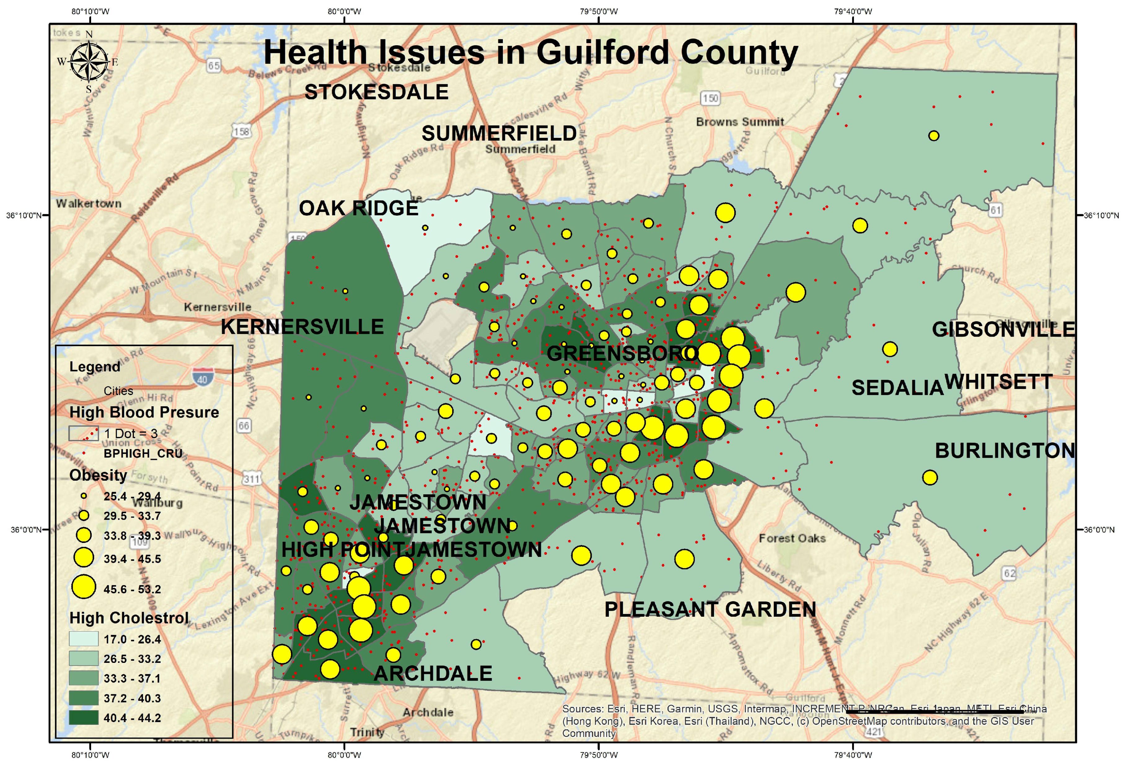
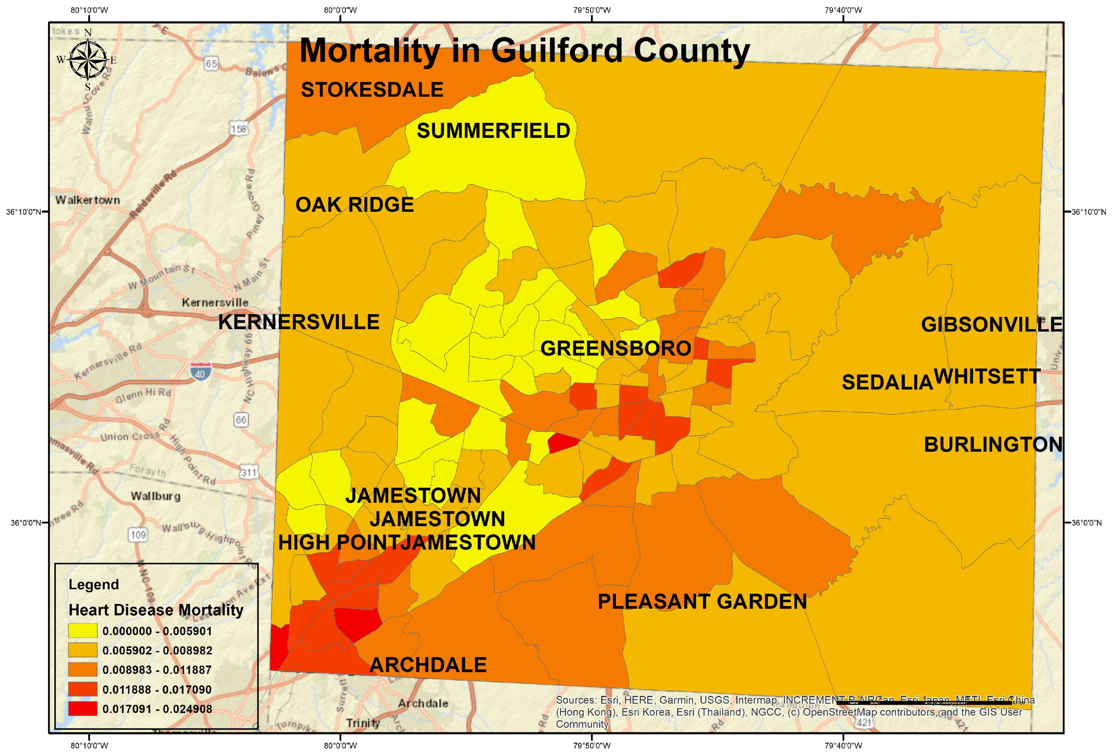
First, we developed the geospatial maps of health (Figure 3) and mortality outcomes for Guilford County. Figure 4 llustrates the geospatial map of heart disease-related mortality rates in Guilford County by percent in each census tract. The descriptive statistics of these health issues are presented in

Table 1. Descriptive statistics.

Statistics	Median Income (USD)	Population	High Blood Pressure	High Cholesterol	Obesity
Mean	51,440.06	3979.78	34.10%	35.70%	35.87%
SD	25,725.97	1498.57	7.59%	5.01%	7.13%
Minimum	14,695.00	1300.00	13.30%	17.00%	25.40%
25% Quartile	33,889.00	2862.00	28.80%	32.80%	29.90%
50% Quartile	47,500.00	3903.00	33.10%	36.20%	34.20%
75% Quartile	60,653.00	5063.00	38.00%	39.60%	53.20%
Maximum	170,625.00	7791.00	55.00%	44.20%	53.20%

.

The mortality rate due to the fact of heart diseases ranged between 0.002% and 0.008% per census tract. Figure 3 shows that there was a high density of obesity and high blood pressure in central Greensboro, Downtown, and Highpoint (outlined in the bounding box). It also coincided with the high density of high cholesterol issues. Notice that the density markers of high cholesterol had higher percentages than hypertension markers. These density maps were developed using the point density tool in ArcGIS software and were overlayed against the obesity density map. Interestingly, the west part of Guilford County showed low obesity numbers. However, high cholesterol and high blood pressure numbers were shown in few census tracts. The distribution of high blood pressure and high cholesterol showed a higher density around Greensboro and Highpoint, too. 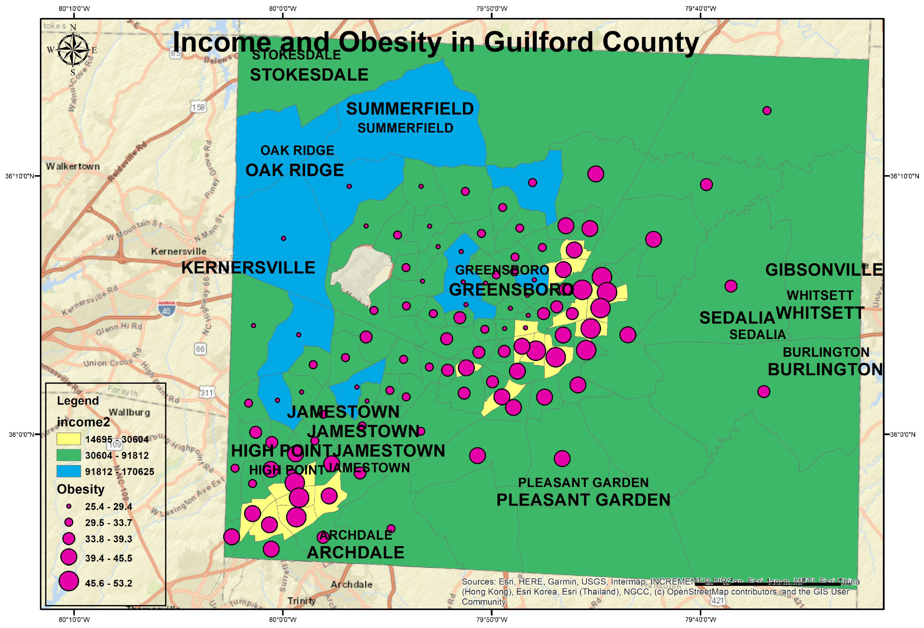Figure 5 shows the mean household income distribution of Guilford County with obesity distribution. A low income was from USD 0 to 30,604, a middle income was between USD 30,604 and 91,812, and a high income was more than USD 91,819 per year [41]. The overall mortality rate map shows a similar pattern in the downtown Greensboro and High Point cities.

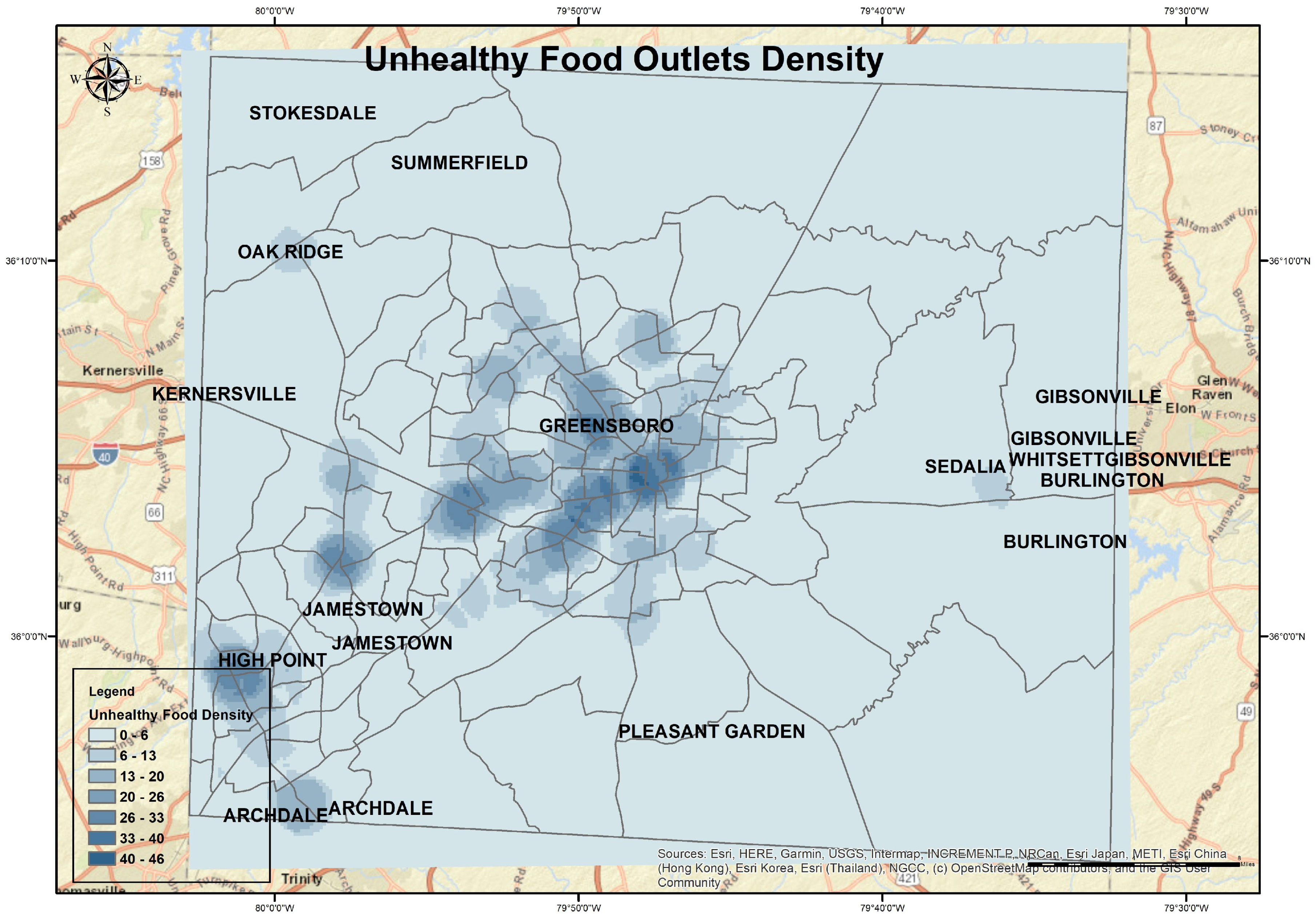
Later, we calculated the total number of healthy and unhealthy food outlets per census tract using the tabulate intersect method, which gave the result in a tabular format. Afterward, the resultant table was joined to the study area using the “Mathematical Join” option. The census tract shapefile was used to find the areas with higher unhealthy food from the intersection of healthy and unhealthy outlet maps in Figure 6 and Figure 7. We then performed spatial analysis using the clip tool in the ArcGIS software to find the number of health issues and the mortality rates in all three food access areas (see

Table 2. The statistics (mean and standard deviation) of health issues, density, income, and mortality rates in each food access area.

	Income (USD)	Population; Acreage	High Cholesterol (Mean, SD)	Obesity (Mean, SD)	Hypertension (Mean, SD)	Mortality (SD)
Food Deserts	41,369.35	105,695, 1418 acres	36.5%, 5.34%	42%, 6.52%	38.8%, 8.38%	0.01%
Food Swamps	51,783.43	189,166, 6485 acres	35%, 4.39%	34%, 6.63%	32%, 6.75%	0.0085%
Food Jungle	60,595.80	13,847, 27,584 acres	37%, 5.58%	35%, 7.84%	36.25%, 7.00%	0.0079%

).

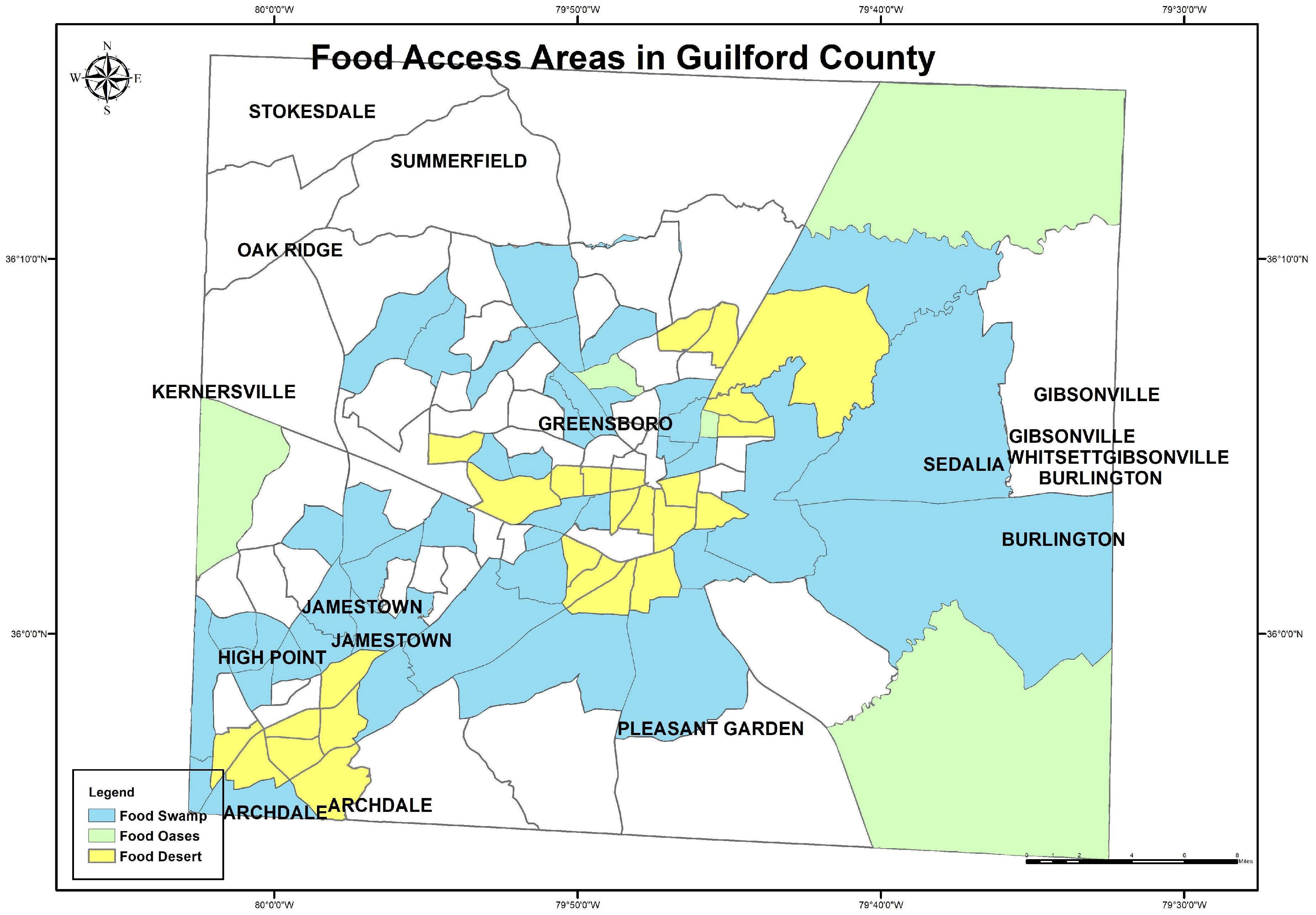
Next, we developed geospatial maps of the three food access areas. Based on healthy food access, Guilford County was divided into three food geographies: food deserts, food swamps, and food oases (Figure 8). Food deserts were measured based on the USDA Economic Research Service definition as the census that had a poverty rate defined as more than 20–30% of its people living more than 1 mile away from a full-service supermarket [42]. In addition, we included where the minority rate was higher, i.e., more than 30% of the total population [43,44]. A food desert is presented in the equation below:

Food desert = low access to supermarkets (the tracts with more than 30% of its people in more than one mile from supermarket) + low car access (households with no personal transportation) + high poverty rate + low income (<USD 30,000 p.a.).

The food desert method started by buffering 1 mile around supermarkets and applying the symmetric differences tool to find the tracts with 30% of the population living one mile away from supermarkets. After that, we applied the intersect tool to the previous layer with the layers of low income, low car access, and high poverty.

The method started by buffering 1 mile around supermarkets and applying the symmetric differences tool to find the 30% of the population that was more than one mile to supermarkets. Afterward, we applied the intersect tool to the previous layer with the layers of income and poverty. Then food deserts showed areas where residents had scarce access to nutritious food. Geospatial mapping of food deserts in Guilford County was developed by identifying areas with the following overlapping characteristics: (i) healthy and unhealthy food density (Figure 6 and Figure 7); (ii) high population density; (iii) high poverty and low income (Figure 5); (iv) low access to transportation. A food desert is a census tract that has less than a 20% poverty rate and at least 30% of its population lives more than one mile from supermarkets.

Afterward, we identified food swamps and food oases. A food swamp had more unhealthy food outlets than healthy outlets, but a food oasis had more healthy than unhealthy food options. Food outlets were categorized as healthy based on fresh food availability such as supermarkets and farmers’ markets. Unhealthy food outlets were packed, and fast food was sold in various places such as restaurants and convenience stores. 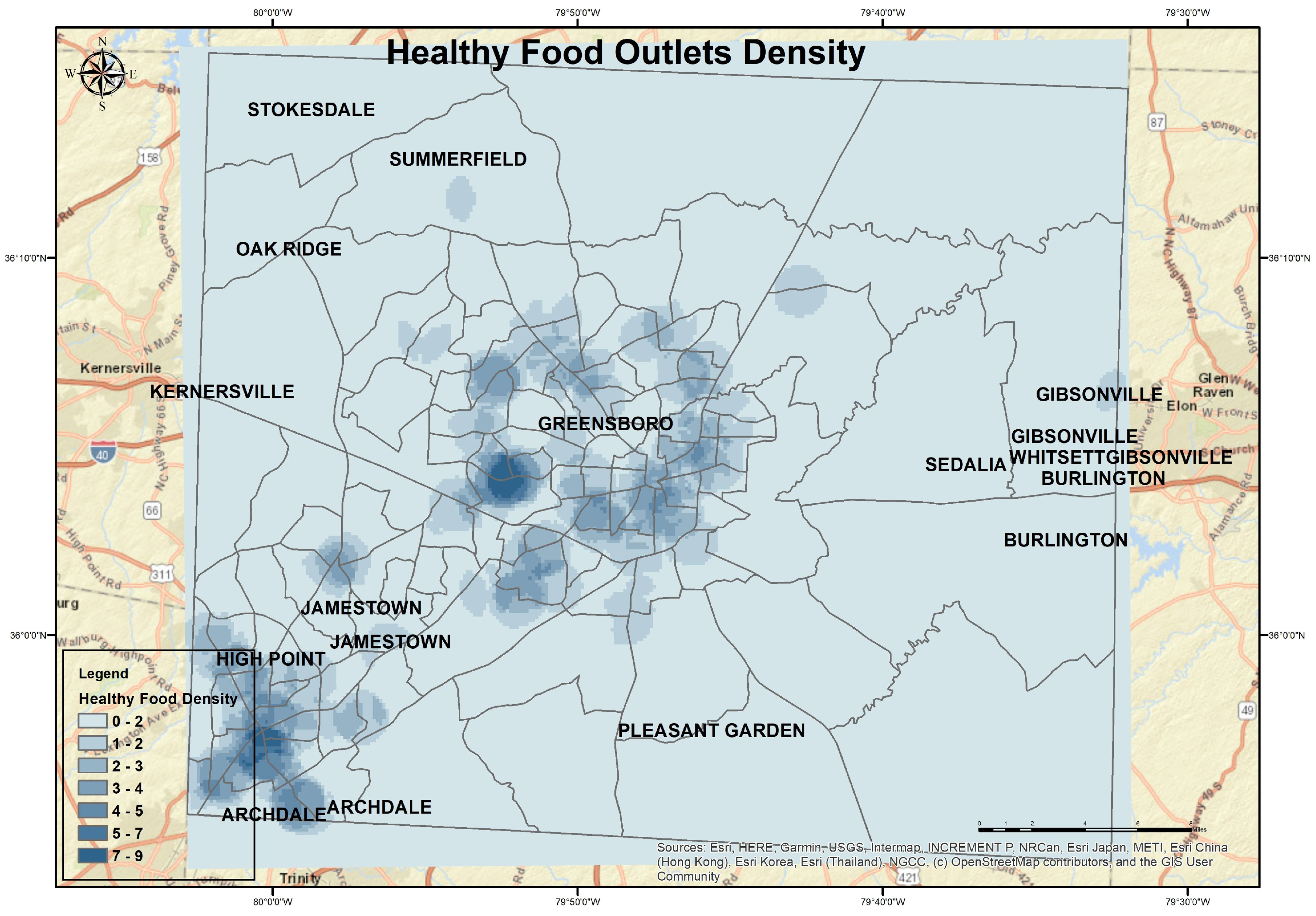To develop the food oases and swamp geo-maps, we categorized healthy and unhealthy food outlets (Figure 6 and Figure 7). The healthy outlets were where fresh vegetables, fruit, and meat were available. This category contained supermarkets, grocery stores, meat markets, farmers’ markets, community gardens, farm road stands, and food parties. Although the second category represented relatively unhealthy food, it comprised convenience stores, dollar stores, and restaurants. We computed the density maps for healthy and unhealthy food outlet stores (Figure 6 and Figure 7) using the region growing density tool. These density maps present the volume of stores for each category. For healthy food outlets, the highest number of stores ranged between 5 and 6 (dark spots in Figure 6), and the lowest was 0−2. For unhealthy food outlets, the highest number of outlets ranged between 40 and 46 stores (dark sports in Figure 7), and the lowest was 0–6.

We computed the descriptive statistics (i.e., mean values and standard deviation) of each health issue in these food access areas for correlation analysis. We used the clip tool additionally to merge the income layer by each food access area to compute the mean household income for Table 2. After developing the overall map showing the three food access areas’ geographies (Figure 8), we compared the health records in each area to determine if there was an effect of healthy food access on health and mortality outcomes. The spatial analysis method showed positive correlations among food outlets and health issues, mortality rates, and income. The results are corroborated in Table 2.

In Table 2, the percentage of the population in food access areas may not provide a clear illustration of the number of people impacted by health issues. For instance, the quantity of 36.5% of the population in food deserts having high blood pressure was 38,578.674, which was higher than 37% of the population in the food jungle (consisting of 5123.39).

2.2. Multioutput Regression and Multiple Linear Regression

We used machine learning techniques to examine the quantitative analytics of population and median income on health issues by specifically applying multioutput regression and multiple linear regressions. Multioutput regressions are regression problems that involve predicting two or more numerical values given several independent variables. The multioutput algorithm is more efficient than the single-output algorithm, because the relations among outputs can be estimated simultaneously by the proposed prediction model. Moreover, application of more than one regression was necessary to compare their results. In this work, we predicted high blood pressure rates, high cholesterol rates, and obesity rates based on the inputs (independent variables) of population, income, and low car access.

The data set was divided into 80% training and 20% testing for multioutput model development. The training set contained eighty-seven (87) observations and twenty-two (22) observations in the testing set, and two different metrics: root mean square (RMS) and R-Squared (R^2) which were used to evaluate the models developed. The implementation of multioutput and multiple linear regression models was conducted with the Sklearn package in Python and MATLAB 2020a, respectively. The default parameters for the multioutput regression models are shown in

Table 3. Regression models’ parameters.

Model	Parameters
Linear Regression Model	copy_X=True, fit_intercept=True, n_jobs=None, normalize=False.
Decision Tress Regression Model	‘ccp_alpha’: 0.0, ‘criterion’: ‘mse’, ‘max_depth’: None,‘max_features’: None, ‘max_leaf_nodes’: None,‘min_impurity_decrease’: 0.0, ‘min_impurity_split’: None, ‘min_samples_leaf’: 1,‘min_samples_split’: 2, ‘min_weight_fraction_leaf’: 0.0, ‘presort’: ‘deprecated’, ‘random_state’: None, ‘splitter’: ‘best’
Random Forest Regression Model	bootstrap=True, ccp_alpha=0.0, critrion=‘mse’, max_depth=None, max_features=‘ato’, max_leaf_nodes=None, max_saples=None, min_impurity_decrease=0.0, min_imprity_split=None, min_samples_leaf=1, min_samples_split=2, min_weight_fraction_leaf=0.0, n_estimtors=100, n_jobs=None, oob_score=False, random_state=None, verbose=0, warm_start=False)
K-Nearest Neighbor Regression Model	lgorithm’: ’auto’, ’leaf_size’: 30,’metric’: ’minkowski’, ’metric_params’: None, ‘n_jobs’: None, ’n_neighbors’: 5, ‘p’: 2, ‘weights’: ‘uniform’

.

The below equation, based on multivariate linear regression, was applied to predict and investigate the relationship between variables, where 49.855 and 0.00029 were the coefficient for the median income variable, 13.233 was the coefficient for car access, and 0.00025 was the coefficient for the interaction between median income and low car access.

y = 49.855 − 0.00029 * MedIncome + 13.236 * Low Car Access − 0.00025 * MedIncome * Low Car Access.

3. Results and Discussion

3.1. Geospaital Correlation

Figure 5 and Figure 6 show geospatial maps of the density of healthy and unhealthy food outlets in Guilford County. In Figure 6, the highest density cluster represents nine healthy and fresh food stores. They were located in the southwest of the county central and the south of the county. In Figure 7, the unhealthy density shows that 42 was the highest number of unhealthy food outlets in a square mile. These clusters were in central Greensboro downtown and Highpoint downtown. Overall, some of the high-density clusters of healthy and unhealthy food were co-located, but the highest cluster for each one was in different areas and varied by four times. With respect to the high-density clusters of unhealthy food that were merged with the defined food desert areas, it appeared as though they had access to more unhealthy food. However, because of other factors (income, population density, and low access to transportation), it represented a food desert where people were unable to access them within a one-mile walking distance. When comparing the mean values of the two food deserts and food oases, it was evident the lower-income household areas had higher obesity, higher hypertension, and higher mortality rates, whereas the high cholesterol mean values were lower in food desert areas. The food swamp areas had low mean values in all health issues in comparison to food jungle areas.

The food access map (Figure 8) and Table 2 both show fewer health issues and mortality rates in food swamps and food oases compared to food deserts due to the better access to healthy food outlets in these two areas. In addition, there was a strong, positive correlation between income and food access, because it facilitates people with the ability to access food stores by car or via another affordable transportation type. Higher access to personal and public transportation showed a negative correlation between health issues and mortality rates. For example, higher-income areas in food oases had fewer health issues and lower mortality rates. The statistics also clearly showed that the food swamps with more unhealthy options were still better than food desert areas with no food access in a mile radius, causing a higher rate of health issues and mortality. These results showed the high numbers of health issues and mortality rates in food desert areas (where more health services, health awareness, and disaster risk preparedness were required for future planning by the county).

The food access map covered only part of the county based on the category qualification applied. However, some areas on the outskirts of the county were not categorized by any of the food access categories (Figure 8), and this could represent a balanced or neutral category of food access area with medium income, medium transportation access, medium food access, and medium population density. Moreover, these areas could have more variance in health statistics and less population density.

3.2. Regression Analysis Results

We conducted machine learning based regression analysis to validate the quantification of dependency relations the food deserts against health factors similar to spatial maps [26,27,28]. We used both linear and nonlinear models such as linear, K-nearest neighbors, decision trees, and random forest. The linear regression independent produced results for a single output at a time, while the other models produced all output at the same time. The aims of using these models were to explore all models, compare their results, and find the more suitable model for food distribution related problems. The Pearson correlation coefficients (R²) matrix indicates degrees of linear association among a set of variables as shown in the correlation matrix heatmap in Figure 9. R² values close to 1 indicate that there is a positive linear relationship between the data columns. Values close to −1 indicate that one column of data has a negative linear relationship to another column of data. The R² values close to or equal to 0 suggest there is no linear relationship between the data columns. The diagonal of the correlation matrix was 1 throughout because there was a positive relationship between all the variables with themselves. It can be observed from the correlation heatmap that there existed a strong correlation between high blood pressure and high cholesterol (R² = 0.82) in Figure 9. In addition, the same could be said for obesity and high blood pressure (R² = 0.77). However, there was a strong, negative correlation between income and obesity (R² = 0.7) in Figure 10. Moreover, there was no relationship between obesity and high cholesterol, as it did not show any negative or positive (R² = 0.34) and substantiated similar to the GIS map in Figure 4.

3.2.1. Multioutput Regression Models

Multioutput regressions are regression problems that involve predicting two or more numerical values given several independent variables. The multioutput algorithm is more efficient than the single-output algorithm because multiple outputs can be estimated simultaneously by the proposed prediction model.

Based on the R-Squared values in

Table 4. R-Squared values of the k-nearest neighbors, random forest, and decision tree for multioutput regression.

	R-Squared
Models	High Blood Pressure	High Cholesterol	Obesity
Linear regression for multioutput Regression	0.375	0.236	0.600
K-nearest neighbors for multioutput regression	0.349	0.045	0.771
Random forest for multioutput regression	0.350	0.054	0.797
Decision tree for multioutput regression	−0.261	−0.806	0.586

and

Table 5. Root mean square error (RMSE) values of k-nearest neighbors, random forest, and decision tree for multioutput regression.

	Root Mean Square Error
Models	High Blood Pressure	High Cholesterol	Obesity
Linear regression for multioutput regression	5.348	3.921	4.417
K-nearest neighbors for multioutput regression	5.50	4.385	3.347
Random forest for multioutput regression	5.457	4.363	3.149
Decision tree for multioutput regression	6.733	5.682	3.792

below, none of the multioutput regression models can be recommended. Nevertheless, the R-Squared values of all four models with obesity as a dependent variable consistently achieved a higher score, with the highest being approximately 79%. The independent variables, namely, median income, low car access, and population, had a significant influence on obesity rate and a negative correlation with high cholesterol.

3.2.2. Multiple Linear Regression Models

Implementation of the multiple linear regression models on the data set was evaluated considering the three dependent variables separately. The value of the coefficient of determination (r-squared) when high blood pressure and high cholesterol were used separately as dependent variables remained significantly low with or without interaction terms. The R-Squared value obtained from these models was below 40%. However, promising results were achieved when “obesity” was used in the multiple linear regression model as a dependent variable.

Table 6. Variables for multiple linear regression model development.

Inputs	Output
Population	Obesity Rate (Figure 2)
Median Income (Figure 6)
Low Car Access

presents the independent variables and dependent variables for the multiple regression model. The predictors or features were transformed to give interaction terms to improve the model (as presented in

Table 7. Results for the multiple linear regression using obesity as a regressor.

Interaction Terms	Normalization	Outlier Removal	Root Mean Square Error	p-Value	R-Squared
No	No	No	4.870	6.10 × 10−18	0.546
Yes	No	No	4.280	7.94 × 10−22	0.660
Yes	Yes	No	0.516	7.48 × 10−25	0.733
Yes	Yes	Yes	0.449	1.78 × 10−28	0.809
Yes	No	Yes	3.110	1.93 × 10−28	0.816

). This means approximately 81% of the variability in the obesity rate (dependent variable) was explained by the independent variables (high blood pressure rate, high cholesterol rate, and obesity) in the multiple linear regression model. There existed a significant interaction between the variables median income and low car and transportation access.

3.2.3. Multivariate Polynomial Regression Models

Implemented on all three variables (i.e., high blood pressure, high cholesterol, and obesity) separately as dependent variables yielded the results. The multivariate polynomial model of the second degree, with “obesity” as the dependent variable, again attained the highest accuracy score of approximately 81%. This was followed by the multivariate polynomial model of the second degree with “high blood pressure” as the dependent, scoring a slightly above 50%. The accuracy for the multivariate polynomial model of the second degree, with “high blood pressure” as the dependent variable, was better than the accuracy obtained for the same variable modeled with multiple linear regression (which fell below 40%). Figure 11 shows the predicted trend versus the test data. The peaks and troughs were very well in sync, using the multivariate polynomial regression for the obesity rate model. In addition, Figure 10 shows the R-Squared and RMSE comparison of multivariate polynomial regression based on second- and third-order polynomial functions. The performance of the model was quite similar in comparison.

4. Conclusions and Future Research

This research investigated the possibility of the geographic correlation of three health issues (i.e., high blood pressure, high cholesterol, and obesity) with food distribution and the statistical correlation with income and car access. These health issues were investigated together to provide a thorough analysis of the chronic health conditions in Guilford County. This study used geospatial technologies and machine learning techniques to provide insights into developing sustainable and healthy communities by examining the presence of food deserts, food swamps, and food oases. We demonstrated how access to healthy food options influenced health and mortality outcomes in one of the largest counties in the state of North Carolina, USA. Specifically, we co-intersected county-level data on representing food access, income distribution, and access to personal and public transportation with data on health or issues and mortality rates.

We started by showing the food outlets’ density and health records in the county. The density measuring technique was an alternative method to creating food access maps. The RFEI measure showed only the quantitative index value and may not have covered all tracts based on the equation’s requirements. Then, we analyzed the health records in the food desert, where people had limited access to healthy food options due to the low income and low transportation access. We also created geospatial maps of food swamps and food oases. Geospatial data presented the distribution of food deserts in Greensboro and Highpoint downtowns; high income distributes in the northwest of Greensboro, in Summerfield, Oakridge, and Kernersville; high density of food outlets, both healthy and unhealthy, in Greensboro and highpoint. The results clearly showed that food swamps had a higher density of unhealthy food outlets than healthy outlets, while a food oasis had a higher density of healthier than unhealthy food options. We then compared the health records in each of these food geographies to examine any influence of healthy food access on health issues.

This study was limited to the study area of Guilford County. The county-level was practical for showing the current stage and helping local decision makers. Involving more counties for comparison would have supported the study’s hypothesis that health issues had a positive correlation with food distribution.

The results of the GIS analysis demonstrated that food deserts with low income, high population density, and low access to transportation were less sustainable, as they showed a high correlation with severe health issues and mortality. Food swamps and oases showed lower health issues and mortality rates compared to food deserts due to the availability of transportation access and income higher than poverty in these areas. The food swamp was a better option than food desert because, nonetheless, the unhealthy food options were accessible. The study’s results presented the correlation of food environment with three health issues, unlike other studies. For instance, a study analyzed the numbers of healthy and unhealthy foods and the rate of obesity and found a correlation with unhealthy food options [45]. However, our study investigated more variables, such as income and car access, which were parts of food access areas.

Food deserts showed greater health issues. This could be related to one of the area’s characteristics: the availability of unhealthy food outlets, high poverty rates, and low access to transportation. Regarding the availability of unhealthy food, some studies showed no association between unhealthy food and health issues such as obesity and hypertension. A study applied statistical analysis to investigate the correlation between unhealthy food options and obesity and hypertension in children but found no significant correlation [46].

Regression models were used to detect relationships and predict results. The application of several regression models was objective in comparing their results. It illustrated the most correlated variables regarding health issues for inclusion in the development plan. Moreover, illustrating these strong variables would benefit stakeholders in directing new plans and investments. Multi-output regression and multiple linear regression analyses were used to examine the correlation between independent and dependent variables in the study area. Multi-output regression is a series of independent linear regressions. There are three outputs and three inputs. The linear regression for the multioutput model coefficients and intercepts is given in the table below (

Table 8. Models’ coefficients.

	Coefficients			Intercept
Models	MedIncome	Car_Access	Population
High blood pressure	−4.04 × 10−5	7.72	−4.18 × 10−4	35.64
High cholesterol	3.79 × 10−5	4.31	−7.89 × 10−4	35.37
Obesity	−1.47	4.05	2.65 × 10−4	41.44

) and the parameters in Table 3. We included different regression models for comparison and evaluated the model with the highest performance. In machine learning, it is not always straightforward that a better model will consistently give higher performances across all distributions of a data set.

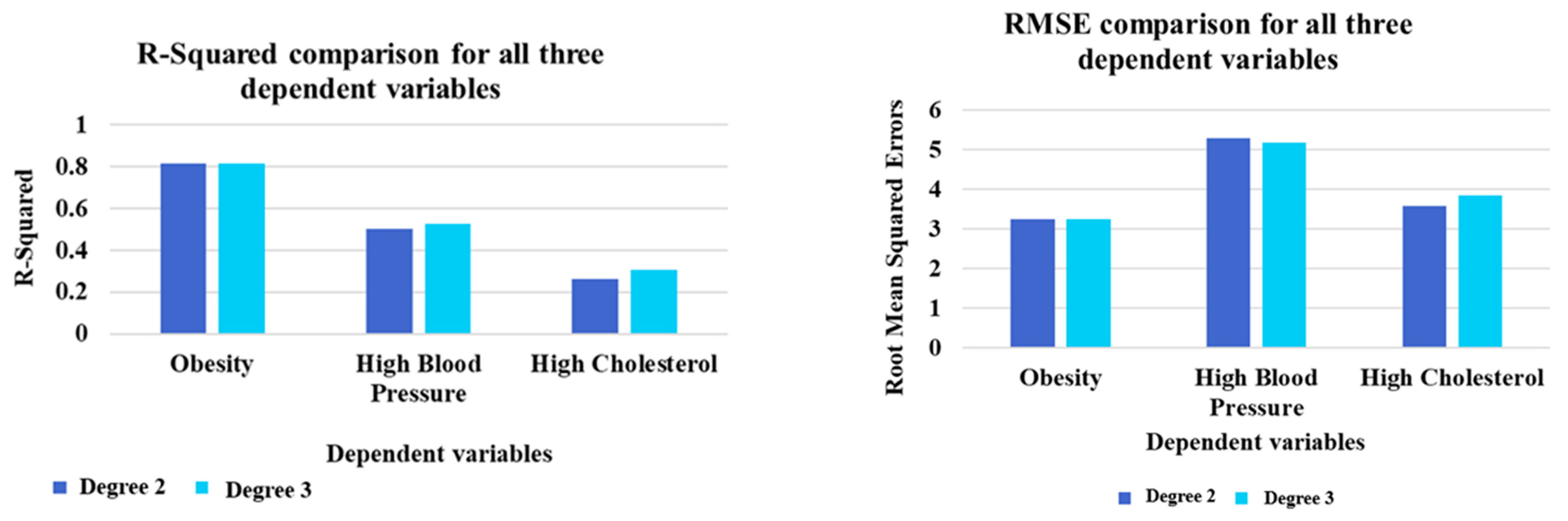
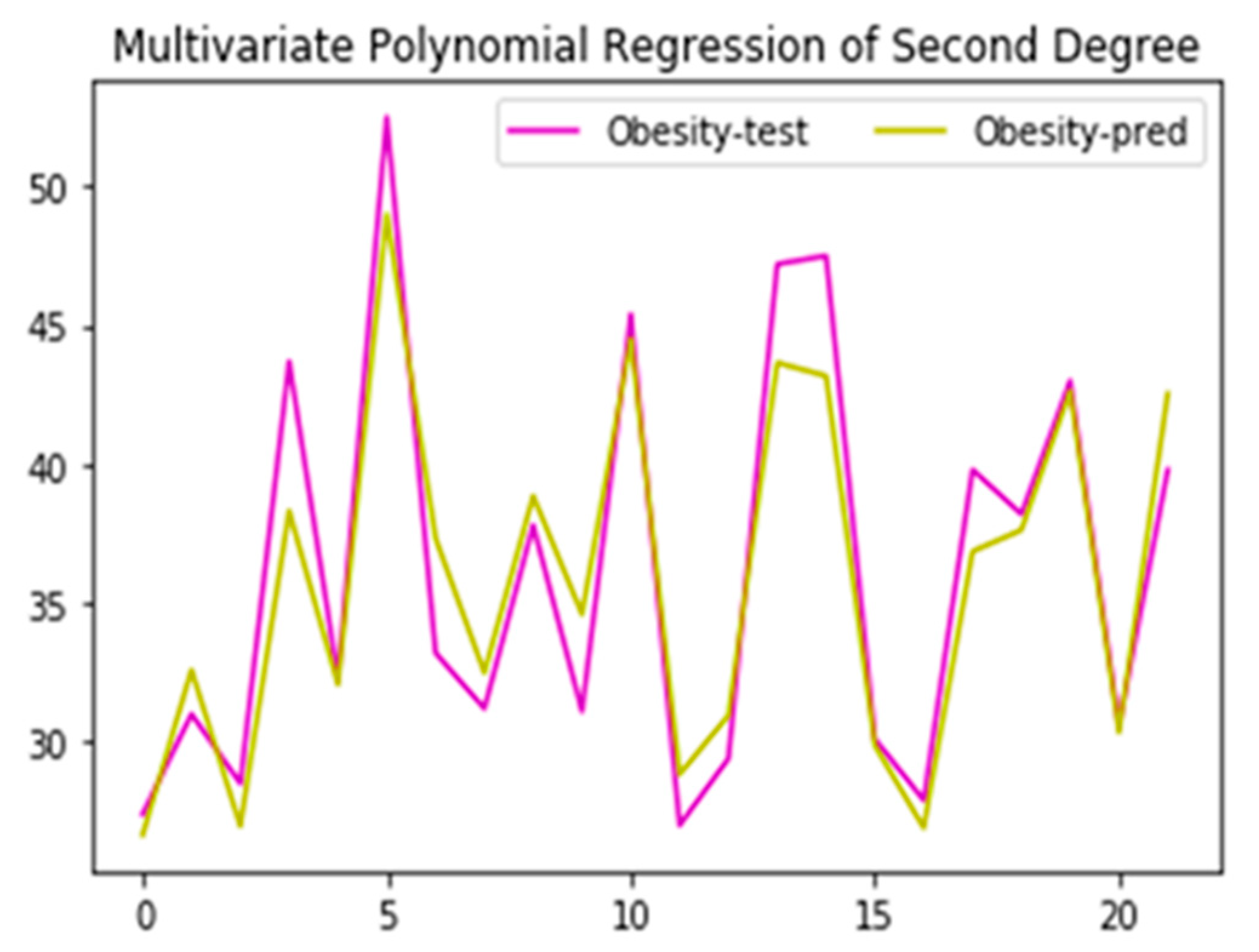
The obesity and high-cholesterol output variables showed high positive and negative correlations (R² = 0.79 and −0.81), respectively, based on the independent variables of low car access, population, and median income. The obesity and high cholesterol variables were modeled using random forest and decision trees for the above performance. In contrast, the linear and nonlinear regression models could only help to predict the dependent variable obesity with an R² value greater than 0.80.

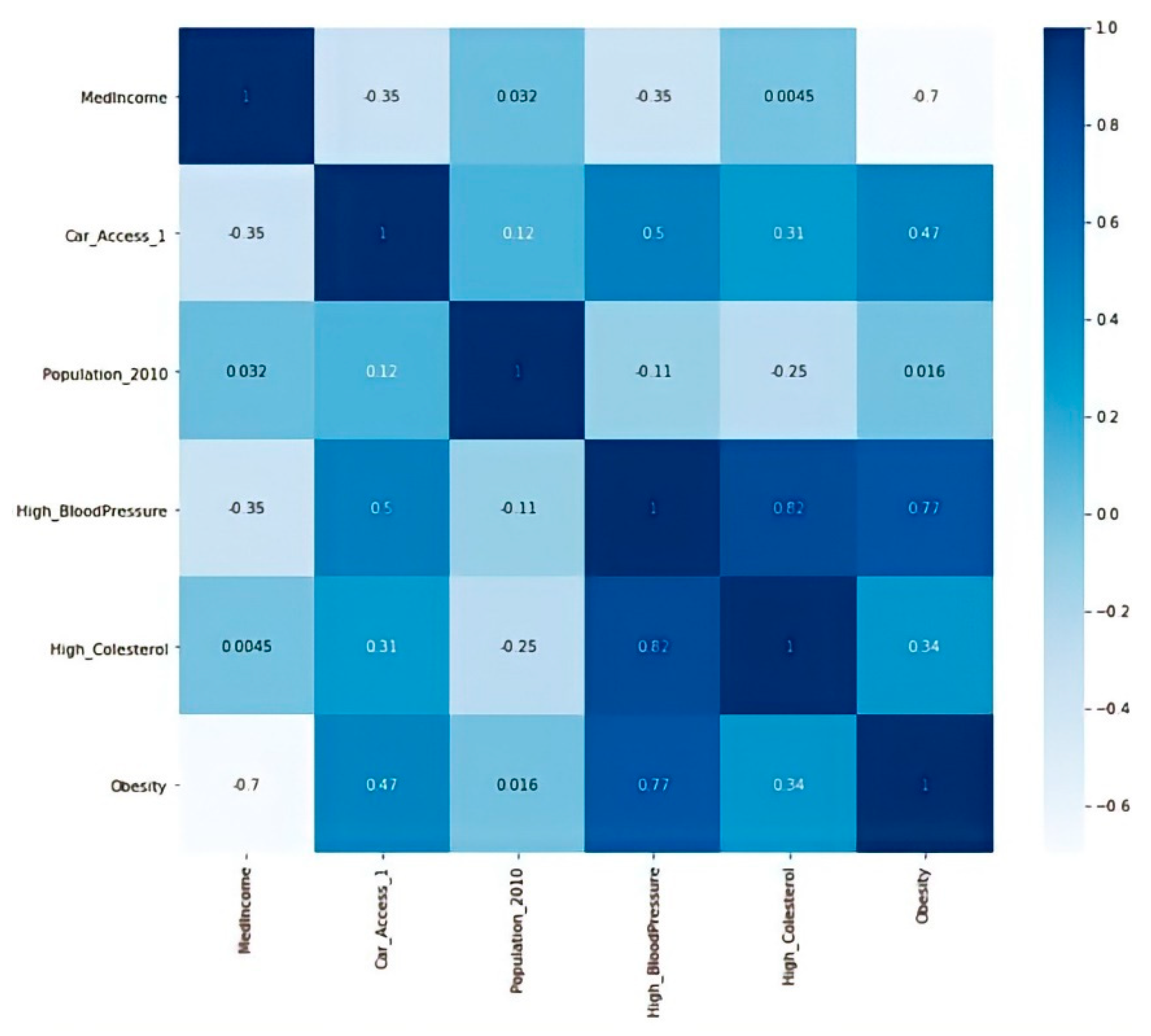
The correlation matrix results illustrated a strong, negative relationship between income and obesity and a positive relationship between independent variables, high blood pressure, and high cholesterol. In addition, it presented the correlation between obesity and income. There was more of a correlation of the independent variable with obesity than between high blood pressure and high cholesterol.

Overall, our results suggested that when compared to food swamps and food oases, food deserts would be the most vulnerable and would probably experience the highest mortality rates in the case of health-related disasters. The presence of such food deserts challenges the sustainable community goals of city and county administrators and directs the need for development in these areas for better future planning.

Future studies may examine the long-term statistical association of food with respect to commercial and governmental policies implemented and its impact on people’s health and conditions. More specific future studies may investigate the low rate of health issues in food swamp areas. Moreover, future research may investigate the increase in health issues and potential cause(s) in various areas over time and recommend possible solutions.