Encoding a Categorical Independent Variable for Input to TerrSet’s Multi-Layer Perceptron

Abstract

The profession debates how to encode a categorical variable for input to machine learning algorithms, such as neural networks. A conventional approach is to convert a categorical variable into a collection of binary variables, which causes a burdensome number of correlated variables. TerrSet’s Land Change Modeler proposes encoding a categorical variable onto the continuous closed interval from 0 to 1 based on each category’s Population Evidence Likelihood (PEL) for input to the Multi-Layer Perceptron, which is a type of neural network. We designed examples to test the wisdom of these encodings. The results show that encoding a categorical variable based on each category’s Sample Empirical Probability (SEP) produces results similar to binary encoding and superior to PEL encoding. The Multi-Layer Perceptron’s sigmoidal smoothing function can cause PEL encoding to produce nonsensical results, while SEP encoding produces straightforward results. We reveal the encoding methods by illustrating how a dependent variable gains across an independent variable that has four categories. The results show that PEL can differ substantially from SEP in ways that have important implications for practical extrapolations. If users must encode a categorical variable for input to a neural network, then we recommend SEP encoding, because SEP efficiently produces outputs that make sense.

1. Introduction

Empirical land-change modeling is a method of revealing the biophysical and anthropogenic patterns of land change, with the goals to understand and to extrapolate the dynamics of a land system, to inform decision-making for land-use planning [1,2]. Spatially-explicit, pattern-based, inductive models of land change rely on mathematical representations of the relationship between independent variables and past land change to extrapolate future land change [2,3]. Machine learning techniques that quantify these mathematical relationships have become popular compared to older parametric techniques, such as logistic regression [4].

The TerrSet software offers machine learning algorithms in its Land Change Modeler (LCM) [5]. Authors have used LCM for many publications [6,7,8,9,10,11]. The Multi-Layer Perceptron (MLP) was the only neural network in LCM for many years until TerrSet’s 2020 version. Our article analyzes the MLP because of its popularity. The MLP calibrates a relationship between independent variables and the transition from an earlier land class to a later land class. The MLP calibrates the relationship using three interconnected layers: the input layer, the hidden layer, and the output layer. Each layer is comprised of individual nodes [12,13,14]. The input nodes for the MLP neural network are the independent variables chosen by the researcher because the researcher believes the variables might be associated with a land cover transition. The MLP uses independent variables on the continuous closed interval from 0 to 1; therefore, all independent variables must be encoded as such. The output of MLP is a soft classification, called the transition potential for a particular land transition. A sigmoidal activation function in the MLP causes a smooth relationship between the encoded independent variable and the transition potential value [5].

Modelers must encode a categorical independent variable so that each category becomes a number on the continuous closed interval from 0 to 1 [15,16]. Sangermano et al. (2012) used likelihoods to encode categorical independent variables [17], but other articles neither explain nor justify their technique for encoding the categorical independent variables [18,19]. We and other authors found scant research concerning the impact of various types of encoding on model calibration [20]. If K is the number of categories in an independent variable, then one-hot encoding transforms each category into a dummy variable for which 0 indicates absence and 1 indicates presence of one of the categories. Thus, one-hot encoding produces a collection of K binary independent variables. Fitkov-Norris et al. (2012) tested four methods of encoding categorical variables in a binary format, including K, K-1, Thermometer K, and Thermometer K-1 encoding [20]. Their first method is one-hot encoding. The thermometer encoding method slightly outperformed K and K-1 encoding in classification accuracy. Binary encoding of a categorical variable that has K categories produces K binary variables, which can exceed computer storage capacity or hinder processing speed. Furthermore, the resulting binary variables are correlated with each other. Therefore, researchers have been searching for alternative encoding methods.

The Land Change Modeler manual recommends that users encode categorical variables based on the concept of Population Evidence Likelihood (PEL) [5]. Let k denote one of the K categories. The PEL for category k is the intersection of category k with the land change between two time points, divided by the size of the land change. Population evidence likelihood assigns the greatest value to the category with the largest change size.

$$\mathrm{Population}\mathrm{Evidence}\mathrm{Likelihood}\mathrm{for}\mathrm{category}k=\frac{\mathrm{size}\mathrm{of}\mathrm{change}\mathrm{on}\mathrm{category}k}{\mathrm{size}\mathrm{of}\mathrm{change}}$$

In contrast, the Geomod land-change simulation model encodes categorical variables based on the concept of population empirical probability (PEP), also known as change intensity [21,22,23]. The PEP for category k is the intersection of category k with the land change between two time points, divided by the size of category k. PEP encoding assigns the greatest value to the category with the greatest change intensity.

$$\mathrm{Population}\mathrm{Empirical}\mathrm{Probability}\mathrm{for}\mathrm{category}k=\frac{\mathrm{size}\mathrm{of}\mathrm{change}\mathrm{on}\mathrm{category} k}{\mathrm{size}\mathrm{of}\mathrm{category} k}$$

Eastman et al. (2005) state that a potential benefit of transforming categorical variables to PEL is that the calculated relationships are independent of the size of each category, and therefore PEL are transferrable across time and space, unlike PEP [4]. The benefit of transforming categorical variables as PEL was a speculation by the authors, who concluded PEL would probably outperform PEP. Their hypothesis was not tested, and we do not understand their reasoning. Furthermore, we could not find literature concerning whether machine learning algorithms find relationships that correspond to PEL, PEP, or some other concept. On the other hand, the PEP transformation of a categorical variable into a continuous transition potential makes intuitive sense to us, because PEP calculates change intensity relative to category size, whereas PEL ignores category size. PEP describes how intensively a gaining dependent variable targets or avoids various categories using the same logic as the transition-level of Intensity Analysis, which is a framework to quantify categorical transitions [23]. The size of change on a category is a product of the category’s size, times the category’s change intensity, thus it makes sense to envision PEP as independent of the category’s size.

To illustrate the fundamental conceptual difference between PEL and PEP, consider a process whereby builders build on a landscape that has various geological categories. If builders consider all geological categories as equally suitable, then builders have no incentive to target or to avoid any particular geological category. If builders were to build on each category with the same intensity, then all categories would have the same PEP while larger categories would have larger PELs. Through this logic, PEP indicates the category’s suitability, while PEL reflects the category’s size. On the other hand, if builders consider some geological categories as more suitable than other geological categories, then builders have an incentive to target the most suitable categories, in which case the more suitable categories would tend to have greater PEPs than the less suitable categories. If the most suitable categories are rare, while the less suitable categories account for the majority of the extent, then builders might build a larger area on the less suitable categories despite the builder’s preference, in which case the less suitable categories would have greater PELs, simply because the less suitable categories are large. It is not immediately clear whether any particular machine learning algorithm tends to learn patterns according to PEL, PEP, or some other criterion.

Our article examines how the MLP neural network in TerrSet’s Land Change Modeler computes transition potentials when the independent variable is categorical. Specifically, our article addresses the question: How should a modeler encode a categorical variable on the continuous closed interval from 0 to 1 for input to the MLP? Our article compares how the MLP neural network produces transition potentials, depending on three encoding methods. We illustrate the concepts using designed data and a practical example from the Plum Islands Ecosystems site of the United States National Science Foundation’s Long Term Ecological Research network.

2. Materials and Methods

2.1. Flow of Methods

Figure 1 shows the flow of steps when using TerrSet’s Land Change Modeler (LCM) with one independent variable that has categories. The legend at the top shows that each color indicates the step’s role in the LCM.

The LCM overlays the land cover maps from the earlier and later time points, to produce a land cover change map. Our manuscript compares three ways to use the land cover change map and the categorical independent variable map to encode the independent variable on the continuous closed interval from 0 to 1. The user must decide whether to encode the categorical independent variable as a collection of binary maps. If so, then the user produces one binary map for each category, where 1 indicates presence and 0 indicates absence of the category. Binary encoding does not use the land cover change map and produces as many binary maps as the number of categories in the independent variable, which consumes computer resources. Alternatively, the user can select an encoding method that produces a single encoded map, where each category receives a number on the continuous closed interval from 0 to 1. Our manuscript compares two ways to use the land cover change map to perform the encoding to a single map.

The Multi-Layer Perceptron reads the encoded independent variable map(s) and the land cover change map to produce a transition potential map for each transition from each losing land cover to each gaining land cover. The transition potential map guides the allocation of the extrapolated change. The LCM uses a Markov procedure that reads the land cover change map and the user-specified future time to extrapolate the size of each transition from a losing land cover to a gaining land cover during the extrapolation time interval. The LCM modifies the later land cover map by converting a number of pixels that matches the extrapolation size for each transition. The LCM allocates changes to the pixels that have the greatest transition potential values. The final output is a map of extrapolated cover change from the calibration interval’s later time to the future time. Our manuscript focuses on how to encode the independent categorical variable, and the encoding’s implications for the MLP’s algorithm to produce the transition potential map, which influences the allocation of extrapolated change.

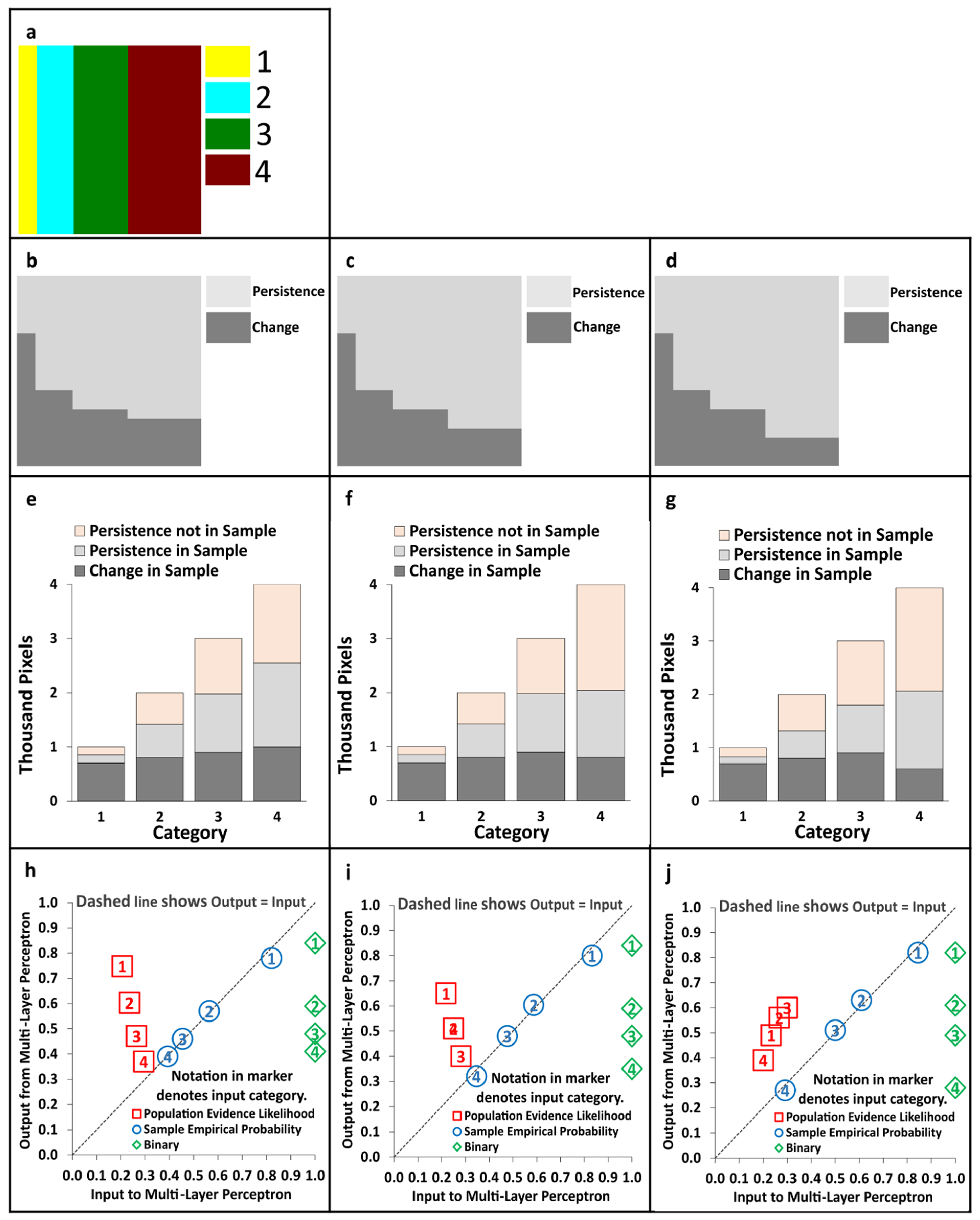
2.2. Theoretical Analysis Illustrated with Designed Data

We designed data with purposeful patterns for three cases to reveal how the MLP neural network uses a categorical variable. Figure 2 shows the designed data, where each image has 100 rows and 100 columns of pixels, which forms 10 thousand pixels. Figure 2a is the independent variable, with four categories named 1, 2, 3, and 4. Category 1 has 1000 pixels; category 2 has 2000 pixels; category 3 has 3000 pixels; category 4 has 4000 pixels. Figure 2b–d shows the dependent variable respectively for cases I, II, and III. The dark grey pixels are the change and the light grey pixels are the persistence between two arbitrary time points. The height of the dark grey region reflects each category’s change intensity, which is the size of change on the category divided by the size of the category. The change intensity decreases from left to right within each of the three cases, as category 1 has the greatest intensity and category 4 has the least intensity. The change intensities of categories 1, 2, and 3 are, respectively, 0.70, 0.40, and 0.30 in all three cases. The change intensity of category 4 shrinks from 0.25 to 0.20 to 0.15 from cases I to II to III. Consequently, cases I, II, and II have change sizes of 3400, 3200, and 3000 pixels, respectively. Figure 2e–g quantifies how the change aligns with the categories for cases I, II, and III. The height of each bar shows the size of each category. The dark grey segment at the bottom of each bar is the change size for each category. The change size remains the same across all three cases on categories 1, 2, and 3. However, the change size on category 4 shrinks from cases I to II to III. Category 4 contains a larger change size than any other category for case I because category 4 is the largest and despite category 4 having the lowest change intensity. Category 4 contains the same change size as category 2 for case II. Category 4 contains a smaller change size than any other category for case III. MLP uses inputs where the number of change pixels equals the number of persistence pixels to avoid the class imbalance problem [24]. However, Figure 2 shows fewer change pixels than persistence pixels, which is typical in practice. Therefore, TerrSet’s MLP uses all of the change pixels and samples an equal number of pixels randomly from the persistence pixels. For example, case I has 3400 change pixels, thus the MLP randomly samples 3400 pixels from the 6600 persistent pixels as input for case I. Consequently, MLP uses 68% of the extent’s ten thousand pixels. Similarly, MLP uses 3200 change pixels and 3200 sampled persistent pixels as input for case II, where MLP uses 64% of the extent’s pixels. MLP uses 3000 change pixels and 3000 sampled persistent pixels as input for case III, where MLP uses 60% of the extent’s pixels.

The light grey segments in Figure 2e–g show the expected number of sampled persistence pixels in each category. The peach-colored segments show the remaining unsampled persistence pixels, which the MLP ignores. Thus, the union of the dark gray and light gray segments in the bars of Figure 2e–g constitutes the input pixels for a run of MLP. MLP then randomly selects half of the input pixels for testing and uses the remaining half for testing the fit for each run of the neural network.

We derived equations to compute the expected number of sampled persistence pixels in each category, which we then used to encode a categorical variable onto the continuous closed interval from 0 to 1 for entry into the MLP.

Table 1. Mathematical notation for Equations (1)–(3).

Symbol	Meaning
k	Identifier for an arbitrary category in the independent variable
K	Number of categories in the independent variable
Ck	Number of change pixels on category k
Dk	Number of persistence pixels on category k
Ek	Expected number of sampled persistence pixels on category k
Sk	Sample Empirical Probability for category k
Pk	Population Evidence Likelihood for category k

gives the notation for the equations.

$$E_k=\left({\displaystyle \sum }_{k=1}^K{C}_k\right)\left\{D_k/\left[{\displaystyle \sum }_{k=1}^K{D}_k\right]\right\}$$

(1)

$$S_k=C_k/\left(C_k+E_k\right)$$

(2)

$$P_k=C_k/\left({\displaystyle \sum }_{k=1}^K{C}_k\right)$$

(3)

Equation (1) computes the expected number of sampled persistence pixels on each category k by multiplying the number of change pixels in the extent times a ratio. The parentheses in Equation (1) contain the number of change pixels in the extent. MLP requires the number of change pixels to equal the number of sampled persistence pixels. The braces in Equation (1) contain a ratio where the numerator is the persistence in category k, while the denominator is the extent’s persistence where the random sampling occurs. Equation (1) generates the light grey segments in Figure 2e–g. Equation (2) uses the dark grey and light grey segments to compute the Sample Empirical Probability for each category k, which is analogous to the population empirical probability in our manuscript’s introduction. However, the Sample Empirical Probability uses the sampled persistence, not the entire persistence. Equation (3) uses the notation to express the Population Evidence Likelihood, as in our manuscript’s introduction. Equation (3) is a function of exclusively the dark grey segments in Figure 2e–g, thus the sampling does not influence Equation (3).

Figure 2h–j compares three encoding methods, where the green diamonds are binary encoding, the blue circles are SEP encoding, and the red squares are PEL encoding. The number within each shape denotes the category. Binary encoding transforms each category to a binary variable, where 1 indicates presence and 0 indicates absence of the category. We ran MLP once for each binary variable. Thus, the green diamonds derive from six MLP runs, consisting of one run for each of categories 1, 2, and 3, plus three runs for the three cases of category 4. SEP requires one MLP run for each of the three cases, where SEP encodes into a single map the four categories onto the continuous closed interval from 0 to 1, which MLP reads in one run for each case. Similarly, PEL requires one MLP run for each of the three cases. A laptop computer completed each run in less than a minute.

Binary encoding is the default method in the profession. Binary encoding makes conceptual sense but requires an onerous amount of computer resources because binary encoding converts one categorical variable of K categories into a collection of K binary variables. The green diamonds in Figure 2h–j shows how binary encoding produces the transition potential as the output for each category. In all of the cases, binary encoding produces the greatest output values for categories that have the greatest change intensity, meaning category 1 has the greatest output value, then category 2, then category 3, and then category 4 has the least output value.

SEP encoding produces output nearly identical to binary encoding, meaning the categories that have more intensive change are the categories that have greater output values. Furthermore, the blue circles are on, or near, the diagonal Output=Input line in the scatter plots of Figure 2h–j. This indicates that the SEP input is nearly identical to the MLP output, implying that SEP gives MLP the answer for which the neural network searches, thus MLP does not need to modify the SEP encoding. The randomness in the sampling causes the sampled number of persistence pixels in each category to deviate slightly from the expected number, which accounts for the slight deviations of some of the blue circles from the Output = Input line.

The PEL encoding is fundamentally different from binary and SEP encoding. Case I in Figure 2h shows a decreasing relationship between the PEL input and MLP output, which indicates that PEL does not give MLP the direct signals for which MLP searches. Figure 2h shows that PEL generates nearly the same outputs as SEP and binary for case I, which is possible because SEP encodes a unique input for each category for case I. However, Figure 2i shows how SEP encoding creates the same input value for categories 2 and 4 because categories 2 and 4 contain the same change size. Therefore, MLP has no opportunity to differentiate between categories 2 and 4, so both categories receive the same output value. Figure 2j shows an even more severe problem with SEP, which relates to the sigmoidal activation function in the neural network, which produces a smooth and possibly non-linear relationship between the input and output values. Sigmoidal functions can constrain overfitting to noisy data, which might be desirable when an independent variable is continuous [25], but our original independent variable is categorical. For Case III in Figure 2j, category 4 has the least SEP and the least output value. Furthermore, category 4 is larger than the other categories; thus, we suspect category 4 has more influence than the other categories in the sigmoidal function. This causes category 4 to pull down the output for category 1 and to push up the output for category 3 relative to cases I and II, even though cases I, II, and III are identical concerning the input data for categories 1, 2, and 3. The sigmoidal function allows one category to influence the output of another category for the SEP encoding, which is an influence that does not exist for the binary encoding and is minor for the PEL encoding.

The output from the binary encoding reflects what the MLP is designed to learn. We suspect that SEP encoding produces output similar to the binary output because SEP gives the MLP the values that MLP is designed to learn. Those values are the change intensities in the sample data. The SEP encoding generates values on the Output=Input line; thus, the smoothing does not have as much effect on SEP as the smoothing has on PEL. The PEL encoding produces two interrelated problems. First, PEL fails to give the intensities that the MLP is designed to learn; second, the sigmoidal smoothing function forces the output of one category to influence the output for other categories, which violates the logic for the analysis of categories.

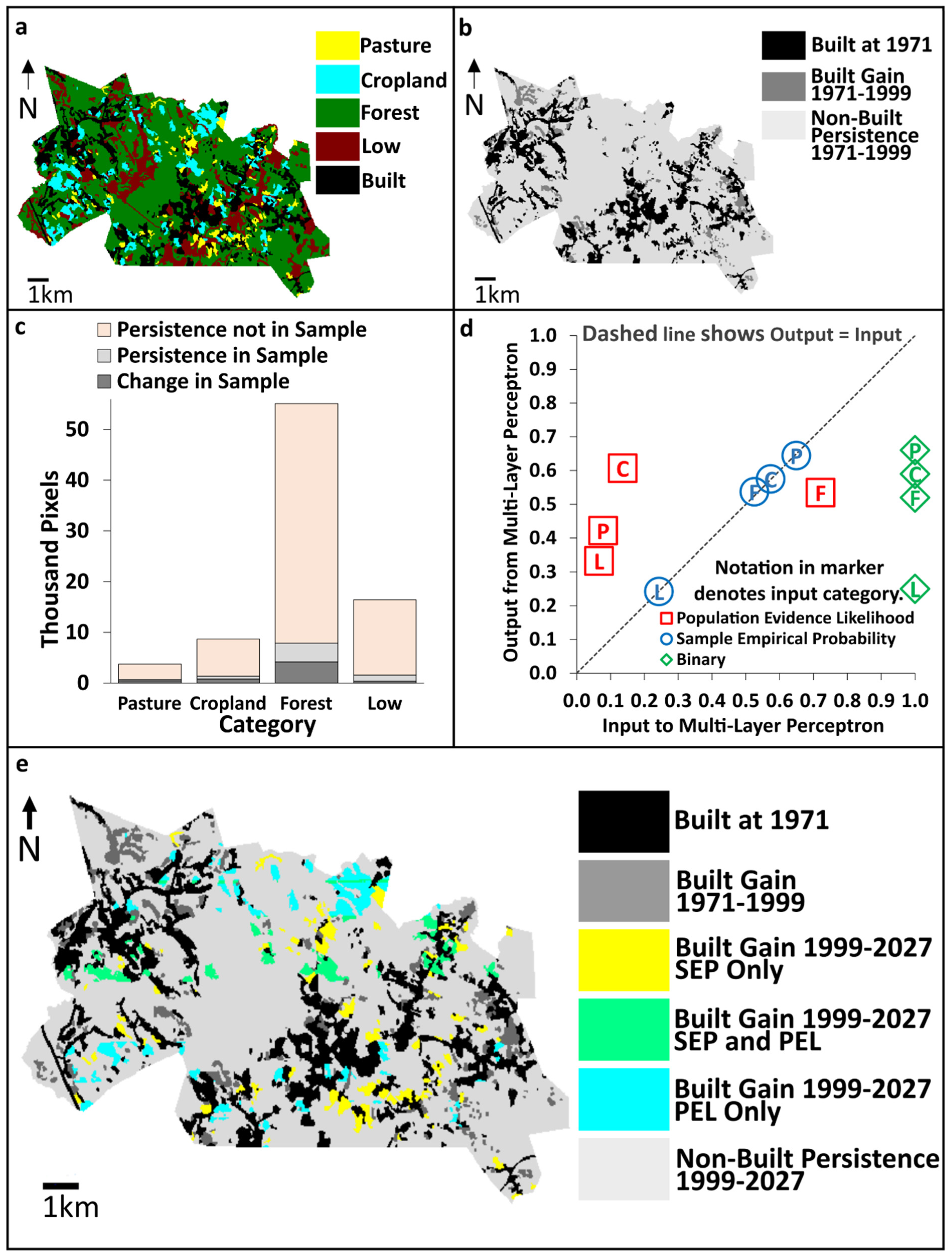
2.3. Practical Application

Figure 3 shows the location of the application to suburban growth in the Plum Island Ecosystems (PIE). The spatial extent is three towns in Massachusetts, USA. Figure 4 shows one independent variable to illustrate the methodological concepts that apply to many possible independent categorical variables, such as soil, zoning, and bins of a continuous variable, such as slope, elevation, and distance to roads. Limited availability of consistent data guided the selection of variables and years. The data derive from maps for the years 1971 and 1999 of the same 21 land categories available from the Commonwealth of Massachusetts [26]. Figure 4a shows the independent categorical variable, which is the 1971 land cover consisting of four categories: Pasture, Cropland, Forest, and Low. These four categories have the potential to transition from 1971 to the Built category because they were not Built at 1971. Low is an aggregation of small land cover categories, most of which have a low transition intensity to Built during 1971–1999. Figure 4b shows the dependent variable of change from non-Built to Built between 1971 and 1999. The Built area at 1971 is excluded from the encoding because the Built area cannot transition to Built. Figure 4c shows the size of each category as the sum of the category’s change, sampled persistence, and unsampled persistence. Forest is the largest category, which is why Forest has the largest change. Cropland has the next largest change, followed by Pasture, then Low. The change size on each category dictates the PEL. Figure 4d shows that the PEL is greatest for Forest, followed by Cropland, Pasture, and least for Low. Figure 4d shows that SEP is greatest for Pasture, followed by Cropland, Forest, and least for Low. We ran MLP as we did with the designed data, meaning with three encoding methods: binary, SEP, and PEL.

TerrSet’s Land Change Modeler simulates change beyond 1999 by extrapolating the quantity distinctly from the allocation of change [5]. A Markov chain extrapolates the quantity of change from the 28-year calibration interval 1971–1999 to the 28-year extrapolation interval 1999–2027. The duration of the calibration interval equals the duration of the extrapolation interval, which makes the Markov chain extrapolation straightforward. MLP’s transition potentials rank the pixels by priority, to allocate Built’s gain. The extrapolation allocates Built’s gain during 1999–2027 to the pixels that have the greatest transition potential values. We generated two sets of transition potential values based on two coding methods: SEP and PEL. Therefore, we make two extrapolations, both of which have the same quantity of Built’s gain during 1999–2027. One extrapolation allocates based on the SEP transition potentials, while the other allocates based on the PEL transition potentials.

3. Results

The results for the PIE data are consistent with the behavior that the designed data demonstrated. For the PIE data, Figure 4d compares the results of the three encoding methods. Binary encoding causes the MLP to produce transition potentials that follow the sequence of the categories’ change intensities. Pasture has the greatest change intensity and receives the greatest transition potential. Low has the least change intensity and receives the least transition potential. SEP encoding causes the MLP to produce transition potentials nearly identical to binary encoding. The SEP input is nearly identical to the output from MLP for each category; thus, the blue circles align with the Output=Input line in Figure 4d. PEL encoding causes the MLP to generate transition potentials different from binary and SEP encoding. PEL encoding causes Cropland to receive the greatest transition potential, followed by Forest, Pasture, then lastly Low. Pasture has the greatest change intensity but the PEL encoding causes Pasture to receive a relatively low transition potential because the sigmoidal function forces Pasture to fit smoothly between the transition potentials for Low and Cropland. The smoothing pulls down the transition potential of Pasture, just as the smoothing pulled down the transition potential for category 1 in the designed data. The smoothing function causes the transition potentials from PEL to follow neither the change intensities nor the change sizes. Repeated runs with the same inputs revealed that MLP’s random sampling does not influence these findings.

Figure 4e shows the extrapolation in PIE during 1999–2027. SEP causes the model to allocate Built’s gain first on all of Pasture, then secondarily on some Cropland. PEL causes the model to allocate all of Built’s gain on Cropland. Consequently, the two allocations have more disagreement than agreement. Figure 4e shows that SEP allocates Built’s gain on the yellow and green regions, while PEL encoding simulates the gain of Built on the green and blue regions. Both allocations show Built’s gain on some of the Cropland.

4. Discussion

4.1. Implications of Results

Some modelers criticize machine learning algorithms as black boxes, where the machine learns, while the modeler does not learn. Our results reveal that the MLP learns by following change intensities, which matches how we and the Geomod model learn about patterns of change. Both binary and SEP encoding reflect categorial intensities. SEP encoding is more efficient than binary encoding because binary encoding increases the number of independent variables. SEP allows the modeler to encode the data as one variable to read into MLP. Our results illustrate that SEP encoding and binary encoding produce similar output values, which rank the categories consistently in sequence of change intensity.

Eastman et al. (2005) proposed PEL to encode a categorical variable while avoiding the creation of a collection of binary variables [4]. SEP meets this same desirable property, which conserves computer resources. The proponents of PEL believed the Multi-Layer Perceptron would benefit from an encoding technique that disconnects the size of each category from the size of change on each category. In contrast, our manuscript indicates that the MLP learns the categorical intensity, which SEP measures by considering the size of the category when accounting for the size of change on the category. Categories that have distinct SEP values might have the same PEL, in which case the MLP has no opportunity to distinguish among categories that differ in terms of category intensity. If PEL encodes the categorical variable, then the effect of MLP’s sigmoidal smoothing function can cause the neural network to not necessarily assign greater output values to the categories with greater change intensities, in which case the smoothing causes nonsensical output.

A comparison among the three designed cases demonstrates that category 1 maintains the same PEL, but the output value for category 1 varies among the cases in response to the PELs of other categories. In cases I and II, category 1 has the least PEL but receives the greatest output value in a decreasing relationship between PELs and output values. In case III, category 4 receives the least output value causing category 1 to receive an output value less than in the previous cases. This change in transition potential for category 1 is an artifact of the sigmoidal function that smooths the relationship between input and output of the MLP. Category 4 is the largest category and thus contributes more pixels to the MLP than category 1, so we suspect that category 4 has a strong influence on the smoothing that corrupts the output for category 1.

The PIE extrapolation exemplifies the key conclusions that the designed cases illustrate. First, the binary and SEP encoding methods produce similar output values. Second, the sigmoidal smoothing function likely influences the output values from PEL in undesirable ways that hinder interpretation. Binary and SEP encoding cause Pasture to receive the greatest output value, whereas PEL encoding causes Pasture to receive the second greatest output value. The smoothing function interacts with the PEL encoding to cause the output value for Pasture to shrink because the PEL for Pasture becomes trapped between the PEL for the categories Low and Cropland. The ranking of categories according to output value influences the allocation when extrapolating change. SEP dictates that Built gains first from Pasture, while PEL dictates that Built gains first from Cropland. The number of pixels extrapolated to transition to Built is larger than the number of pixels of Pasture; therefore, the SEP allocates Built’s gain on all of Pasture and some of Cropland, because Cropland has the second-greatest transition potential. PEL allocates all of Built’s gain to Cropland, thus the two extrapolations intersect on portions of Cropland, while the two extrapolations disagree more than they agree.

Some researchers have been tempted to judge an extrapolation model by its predictive power, through validation with an empirical reference map at the extrapolated time point. Varga et al. (2019) explain several reasons why that is a flawed criterion by which to judge an extrapolation model [27]. Most importantly, the purpose of an extrapolation model is to capture the signal of change during a calibration time interval and then to extrapolate the signal during the extrapolation time interval, to help to understand the implications of a continuation of historic trends. If the empirical trends during the calibration interval are not consistent with the empirical trends during the extrapolation interval, then validation will show errors even when the model accomplishes what the model is designed to do. Validation shows the ability of a model to predict the future, which is not the purpose of the MLP. The MLP is designed to characterize the relationship between the dependent and independent variables that the MLP reads. Our manuscript uses methods to assess how efficiently MLP accomplishes its goal for the coding of a categorical independent variable.

4.2. Next Steps

Our manuscript examines the behavior of the MLP by using designed data and a practical application. We used our understanding of machine learning algorithms to guide our research. However, we did not examine the computer code of the MLP as programmed into TerrSet. Thus, our analysis begs the following questions for future research.

First, the scatter plots in Figure 2 and Figure 4 show that the SEP input nearly equals the neural network’s output for each category. The likely reason for the slight deviations between SEP input and SEP output is that the randomization in the sampling can cause slight deviations between the randomly selected number and the expected number of persistence pixels in the sample for each category. If SEP is the value that the neural network is designed to learn for each category, then SEP already gives the answer that the neural network seeks. Therefore, why should modelers use the neural network when modelers could quickly compute what the neural network takes time to learn?

Second, the neural network’s sampling uses less information than is easily available, which is a wasted opportunity. The neural network uses random sampling to select a subset of the persistence. The motivation for the sampling is to generate input data where the number of change pixels is equal to the number of persistence pixels. However, the sampling constitutes a loss of information and an introduction of randomness, merely to surrender to the requirements of the neural network’s complex fitting algorithm. Thus, again we ask, why should modelers use the neural network when a more direct, comprehensive, and interpretable computation is available?

Third, the combination of Equations (1) and (2) implies that SEP for each category is a function of four factors: the category’s number of change pixels, the category’s number of persistence pixels, the extent’s number of change pixels, and the extent’s number of persistence pixels. The third and fourth factors imply that pixels outside a category affect the category’s SEP, which renders SEP challenging to interpret.

Table 2. Mathematical notation for Equations (4)–(7).

Symbol	Meaning
k	Identifier for an arbitrary category in the independent variable
K	Number of categories in the independent variable
Ck	Number of change pixels in category k
Dk	Number of persistence pixels in category k
R	Extent’s proportion of change
Gk	Population empirical probability for category k
Ek	Expected number of sampled persistence pixels in category k
Sk	Sample Empirical Probability for category k

contains notation for Equations (4)–(7), which give insight into the interpretation of SEP. Equation (4) expresses the extent’s change prevalence, which is the ratio of the number of change pixels to the sum of change and persistence pixels. We assume the number of change pixels is positive, thus, R is positive; otherwise, the calibration procedure would have no signal of change. Equation (5) expresses the population empirical probability for category k, denoted as G_k because the Geomod model uses this computation [21]. Equation (5) implies Equation (6), which assumes G_k > 0 to avoid division by zero. Equation (7) begins with Equation (2), and then uses algebra and substitution with Equations (4)–(6) to express S_k as a function of G_k and R.

$$0<R=\frac{{{\displaystyle \sum }}_{k=1}^K{C}_k}{{{\displaystyle \sum }}_{k=1}^K\left(C_k+D_k\right)}\le 1$$

(4)

$$0\le G_k=\frac{C_k}{C_k+D_k}\le 1$$

(5)

$$D_k=\frac{C_k}{G_k}-C_k=\frac{C_k-G_k{C}_k}{G_k}=\frac{\left(1-G_k\right)C_k}{G_k}\mathrm{when}{G}_k\text{≠}0$$

(6)

$$\begin{array}{ll}{S}_k=\frac{C_k}{C_k+E_k}& =\frac{C_k}{C_k+\left({\displaystyle \sum {}_{k=1}^K}\right)\left\{D_k/\left[{\displaystyle \sum {}_{k=1}^K{D}_k}\right]\right\}}\\ & =\frac{\left[{\displaystyle \sum {}_{k=1}^K{D}_k}\right]C_k}{\left[{\displaystyle \sum {}_{k=1}^K{D}_k}\right]C_k+\left({\displaystyle \sum {}_{k=1}^K{C}_k}\right)\left\{D_k\right\}}=\frac{\left(1-R\right)C_k}{\left(1-R\right)C_k+R{D}_k}\\ & =\frac{\left(1-R\right)C_k}{\left(1-R\right)C_k+R\frac{\left(1-G_k\right)C_k}{G_k}}=\frac{G_k\left(1-R\right)}{G_k\left(1-R\right)+R\left(1-G_k\right)}\\ & =\frac{G_k\left(1-R\right)}{G_k\left(1-R\right)+R-R{G}_k}=\frac{G_k\left(1-R\right)}{G_k\left(1-2R\right)+R}\\ & =\frac{1-R}{1-2R+\left(R/G_k\right)}\end{array}$$

(7)

The ratio (R/G_k) in the final expression of Equation (7) shows that S_k increases as G_k increases. As G_k approaches 0, S_k approaches 0. If G_k = R then S_k = 1/2. As G_k approaches 1, S_k approaches 1. If C_k = 0, then S_k = G_k = 0. Therefore, S_k is a one-to-one function of G_k on the continuous closed interval from 0 to 1, thus S_k has information equivalent to G_k. The implication is that the MLP neural network uses random sampling and a complex process to learn the same information that Geomod computes more intuitively without random sampling. Geomod lacks smoothing between the categories because smoothing is not appropriate for a categorical variable. MLP’s smoothing has no influence with binary encoding, little influence with SEP encoding, and potentially corruptive influence with PEL encoding. Geomod and SEP follow the same type of logic based on categorical intensities, but Geomod uses G_k, which has a more direct interpretation concerning the calibration data than SEP. The set of G_k gives the categorical intensities in the calibration data, while SEP does not. MLP requires sampling that makes SEP deviate from the categorical intensities in the calibration data. Therefore, the same question applies, why should modelers use the neural network when a more direct, comprehensive, and interpretable computation is available?

Fourth, the profession needs additional research regarding the smoothing influence of the sigmoidal activation function. We can imagine an infinite number of ways to smooth a curve, while it is unclear under what conditions particular types of smoothing are desirable. If the software does not allow the user to set the smoothing separately from other parameters that influence the MLP’s output, then it is difficult to isolate the influence of the smoothing. If we could control the smoothing, then we could address the following question. If smoothing were absent while each category has a unique PEL, then would PEL encoding generate output identical to both SEP and binary encodings?

Fifth, our manuscript analyzes three ways of encoding a categorical variable onto the continuous closed interval from 0 to 1. We found that MLP learns a relationship that relates to the intensity of land change at various places along that continuum. However, it is not clear how to compute the change intensity for a continuous variable. One approach is to break the continuous variable into a set of ordered bins, as a histogram does, then treat the continuous variable as a categorical variable; thus, our manuscript’s insights might apply. What are the implications of our manuscript’s insights for how a neural network learns when the original input variable is continuous, such as distance to roads?

Our sixth question for future research concerns whether the insights we have revealed for the MLP apply to other machine learning algorithms. Do our insights concerning intensities, sampling, and smoothing apply to algorithms such as Decision Forest, Weighted Normalized Likelihood, Support Vector Machines, and SimWeight, which TerrSet recently included in its Land Change Modeler?

5. Conclusions

If modelers use a neural network to fit an independent categorical variable, then we recommend users adopt the Sample Empirical Probability (SEP) encoding method, because SEP efficiently generates interpretable results, while avoiding the creation of a burdensome number of correlated binary variables. SEP allows researchers to encode a categorical independent variable as a single variable on the continuous closed interval from 0 to 1 for input to the Multi-Layer Perceptron neural network. We recommend that TerrSet’s Land Change Modeler discontinue its recommendation to transform a categorical variable into Population Evidence Likelihood, and instead, recommend transforming a categorical variable into SEP.

References

1. Costanza, R.; Ruth, M. Using dynamic modeling to scope environmental problems and build consensus. Environ. Manag. 1998, 22, 183–195. [Google Scholar] [CrossRef] [PubMed]
2. Verburg, P.; Schot, P.; Dijst, M.; Veldkamp, A. Land-use change modeling: Current practice and research priorities. GeoJournal 2004, 61, 309–324. [Google Scholar] [CrossRef]
3. Mas, J.; Kolb, M.; Paegelow, M.; Camacho Olmedo, M.T.; Houet, T. Inductive pattern-based land use/cover change models: A comparison of four software packages. Environ. Model. Softw. 2014, 51, 94–111. [Google Scholar] [CrossRef] [Green Version]
4. Eastman, J.R.; Van Fossen, M.; Solorzano, L. Transition potential modeling for land cover change. In GIS, Spatial Analysis and Modeling; ESRI Press: Redlands, CA, USA, 2005; pp. 339–368. [Google Scholar]
5. Eastman, J.R. TerrSet Geospatial Monitoring and Modeling System; Clark University: Worcester, MA, USA, 2020; Available online: https://clarklabs.org (accessed on 1 October 2021).
6. Areendran, G.; Raj, K.; Mazumdar, S.; Puri, K.; Shah, B.; Mukerjee, R.; Medhi, K. Modeling REDD+ baselines using mapping technologies: A pilot study from Balpakram-Baghmara Landscape (BBL) in Meghalaya, India. Int. J. Geoinformat. 2013, 9, 61–71. [Google Scholar] [CrossRef]
7. Gong, H.; Simwanda, M.; Murayama, Y. An Internet-based gis platform providing data for visualization and spatial analysis of urbanization in major Asian and African cities. ISPRS Int. J. Geo-Inf. 2017, 6, 257. [Google Scholar] [CrossRef] [Green Version]
8. Kefi, M.; Mishra, B.K.; Kumar, P.; Masago, Y.; Fukushi, K. Assessment of tangible direct flood damage using a spatial analysis approach under the effects of climate change: Case study in an urban watershed in Hanoi, Vietnam. ISPRS Int. J. Geo-Inf. 2018, 7, 29. [Google Scholar] [CrossRef] [Green Version]
9. Megahed, Y.; Cabral, P.; Silva, J.; Caetano, M. Land cover mapping analysis and urban growth modelling using remote sensing techniques in greater Cairo Region—Egypt. ISPRS Int. J. Geo-Inf. 2015, 4, 1750. [Google Scholar] [CrossRef] [Green Version]
10. Nath, B.; Wang, Z.; Ge, Y.; Islam, K.; Singh, R.P.; Niu, Z. Land use and land cover change modeling and future potential landscape risk assessment using Markov-CA model and analytical hierarchy process. ISPRS Int. J. Geo-Inf. 2020, 9, 134. [Google Scholar] [CrossRef] [Green Version]
11. Rimal, B.; Zhang, L.; Keshtkar, H.; Haack, B.N.; Rijal, S.; Zhang, P. Land Use/land cover dynamics and modeling of urban land expansion by the integration of cellular automata and Markov chain. ISPRS Int. J. Geo-Inf. 2018, 7, 154. [Google Scholar] [CrossRef] [Green Version]
12. Pijanowski, B.; Shellito, B.; Bauer, M.; Sawaya, K. Calibrating a neural network-based urban change model for two metropolitan areas of the upper Midwest of the United States. Int. J. Geogr. Inf. Sci. 2005, 19, 197–215. [Google Scholar] [CrossRef]
13. Rosenblatt, F. The perceptron: A probabilistic model for information storage and organization in the brain. Psychol. Rev. 1958, 65, 386–408. [Google Scholar] [CrossRef] [Green Version]
14. Rumelhart, D.E.; Hinton, G.E.; Williams, R.J. Learning internal representations by error propagation. In Parallel Distributed Processing: Explorations in the Microstructure of Cognition, Vol. 1: Foundations; MIT Press: Cambridge, MA, USA, 1986; pp. 318–362. [Google Scholar]
15. Potdar, K.; Pardawala, T.; Pai, C. A Comparative study of categorical variable encoding techniques for neural network classifiers. Int. J. Comput. Appl. 2017, 175, 7–9. [Google Scholar] [CrossRef]
16. Hancock, J.T.; Khoshgoftaar, T.M. Survey on categorical data for neural networks. J. Big Data 2020, 7, 28. [Google Scholar] [CrossRef] [Green Version]
17. Sangermano, F.; Toledano, J.; Eastman, J.R. Land cover change in the Bolivian Amazon and its implications for REDD+ and endemic biodiversity. Landsc. Ecol. 2012, 27, 571–584. [Google Scholar] [CrossRef]
18. Bradley, A.V.; Rosa, I.M.D.; Brandão, A.; Crema, S.; Dobler, C.; Moulds, S.; Ahmed, S.E.; Carneiro, T.; Smith, M.J.; Ewers, R.M. An ensemble of spatially explicit land-cover model projections: Prospects and challenges to retrospectively evaluate deforestation policy. Model. Earth Syst. Environ. 2017, 3, 1215–1228. [Google Scholar] [CrossRef]
19. Zheng, X.; He, G.; Wang, S.; Wang, Y.; Wang, G.; Yang, Z.; Yu, J.; Wang, N. Comparison of machine learning methods for potential active landslide hazards identification with multi-source data. ISPRS Int. J. Geo-Inf. 2021, 10, 253. [Google Scholar] [CrossRef]
20. Fitkov-Norris, E.; Vahid, S.; Hand, C. Evaluating the impact of categorical data encoding and scaling on neural network classification performance: The case of repeat consumption of identical cultural goods. In Engineering Applications of Neural Networks; Jayne, C., Yue, S., Iliadis, L., Eds.; Springer: Berlin/Heidelberg, Germany, 2012; pp. 343–352. [Google Scholar]
21. Pontius, R.G., Jr.; Cornell, J.D.; Hall, C.A.S. Modeling the spatial pattern of land-use change with GEOMOD2: Application and validation for Costa Rica. Agric. Ecosyst. Environ. 2001, 85, 191–203. [Google Scholar] [CrossRef] [Green Version]
22. Andaryani, S.; Sloan, S.; Nourani, V.; Keshthar, H. The utility of a hybrid GEOMOD-Markov Chain model of land-use change in the context of highly water-demanding agriculture in a semi-arid region. Ecol. Inform. 2021, 64, 101332. [Google Scholar] [CrossRef]
23. Quan, B.; Pontius, R.G., Jr.; Song, H. Intensity analysis to communicate land change during three time intervals in two regions of Quanzhou City, China. GIScience Remote Sens. 2020, 57, 21–36. [Google Scholar] [CrossRef]
24. Amadlou, M.; Karimi, M.; Pontius, R.G., Jr. A new framework to deal with the class imbalance problem in urban gain modeling based on clustering and ensemble models. Geocarto Int. 2021. [Google Scholar] [CrossRef]
25. Hsieh, W.W. Machine Learning Methods in the Environmental Sciences: Neural Networks and Kernels; Cambridge University Press: Cambridge, UK, 2009. [Google Scholar] [CrossRef] [Green Version]
26. Commonwealth of Massachusetts. 2016. Available online: https://www.gismanual.com/lookup/MassGISLandUse.html (accessed on 1 October 2021).
27. Varga, O.G.; Pontius, R.G., Jr.; Singh, S.K.; Szabó, S. Intensity analysis and the figure of merit’s components for assessment of a Cellular AutomataMarkov simulation model. Ecol. Indic. 2013, 101, 933–942. [Google Scholar] [CrossRef]
Figure 1. Flow diagram of the Land Change Modeler when using one independent variable that shows categories. Our manuscript addresses the user decision concerning the method of encoding a categorical independent variable and the decision’s implications for the transition potential map and the subsequent extrapolated land cover map.
Ijgi 10 00686 g001
Figure 2. Designed data shows that Sample Empirical Probability is robust to smoothing, unlike Population Evidence Likelihood. (a) The independent categorical variable. (b) Case I dependent variable, where change intensity declines from categories 1 to 4. (c) Case II dependent variable, where the change intensity of category 4 shrinks from case I. (d) Case III dependent variable, where the change intensity of category 4 shrinks from case II. (e) Case I bars, where category 4 has the largest change size. (f) Case II bars, where category 4 has the same change size as category 2. (g) Case III bars where category 4 has the smallest change size. (h) Case I scatter plot, where the three encoding methods produce similar output. (i) Case II scatterplot, where PEL renders the MLP unable to distinguish between categories 2 and 4. (j) Case III scatter plot, where PEL produces a category ranking different from the other encoding methods.
Ijgi 10 00686 g002
Figure 3. The Plum Island Ecosystems site consisting of the towns of Topsfield, Hamilton, and Wenham in northeastern Massachusetts, USA.
Ijgi 10 00686 g003
Figure 4. PIE data demonstrates that Sample Empirical Probability and Population Evidence Likelihood produce different results when used to extrapolate into the future. (a) The independent variable of land cover at 1971. (b) The dependent variable of change from non-Built at 1971 to Built at 1999. (c) Sizes of the categories, where Pasture has the greatest change intensity, while Forest has the largest change size. (d) Scatterplot, where each marker contains the first letter of the category. (e) Comparison of the allocation from the Sample Empirical Probability (SEP) and Population Evidence Likelihood (PEL) for the extrapolation from 1999 to 2027, where SEP favors Pasture first then Cropland, while PEL favors Cropland.
Ijgi 10 00686 g004