HiIndex: An Efficient Spatial Index for Rapid Visualization of Large-Scale Geographic Vector Data

Abstract

In the big data era, rapid visualization of large-scale vector data has become a serious challenge in Geographic Information Science (GIS). To fill the gap, we propose HiIndex, a spatial index that enables real-time and interactive visualization of large-scale vector data. HiIndex improves the state of the art with its low memory requirements, fast construction speed, and high visualization efficiency. In HiIndex, we present a tile-quadtree structure (TQ-tree) which divides the global geographic range based on the quadtree recursion method, and each node in the TQ-tree represents a specific and regular spatial range. In this paper, we propose a quick TQ-tree generation algorithm and an efficient visualization algorithm. Experiments show that the HiIndex is simple in structure, fast in construction, and less in memory occupation, and our approach can support interactive and real-time visualization of billion scale vector data with negligible pre-treatment time.

1. Introduction

Geographic vector data plays an important role in urban planning, land use, environmental factor analysis, and many other fields. Visualization can make intricate data more intuitive to human readers, which is important to discover implicit information and support further decisions [1]. To display geographic vector data on the screen, it is often necessary to rasterize the vector objects. At the same time, points, linestrings, and polygon edges should be visualized with a certain pixel width, and the process will be extremely time-consuming when the data size increases dramatically. In our previous work, we proposed a display-driven computing model (DisDC) [2]. DisDC directly takes pixels as the calculation units to get the final display effects. Based on the core idea of DisDC, the visualization of geographic vector data can be converted into the key process for determining whether the spatial location of a pixel is within a certain pixel width of the boundary of vector objects. To achieve a quick determination of the above spatial relationship between the pixel and vector objects, a common approach is to use existing spatial indexing methods to indirectly determine the spatial relationship through the spatial retrieval results.

Spatial indexing methods are an important means for massive data retrieval. There are various spatial indexing methods for different application scenarios [3], typical index structures include the grid index [4,5], the KD-tree index [6], the quadtree index [7], and the R-tree index [8], as well as the improvement, union, and variation of the above indexes. With the development of computer hardware, the distributed storage system is widely used in the organization and management of spatial data [9,10,11,12]. Distributed indexes significantly improve the efficiency of data retrieval. Through parallel data partitioning and parallel spatial query, several traditional spatial indexing algorithms have been implemented in a parallel environment [10,13,14]. However, current spatial indexing methods mainly focus on some specific scenarios: the balanced tree index structure ensures query performance but brings large construction and update costs; the unbalanced tree structure ensures the efficiency of construction and update, but it is difficult to deal with the problem of data skew in the clustering model. Although the adoption of distributed technology improves the index retrieval efficiency, it increases the communication overhead between cluster nodes and makes the index structure more complex, and the index must fully consider the overall framework of the distributed system and the way of organizing data, which increases the cost of index construction and fails to achieve high-performance in data pre-processing and visualization at the same time.

We have designed a rapid visualization method called HiVision [15]. It enables fast discrimination of the above spatial relationship by constructing an R-tree spatial index on the vector data. HiVision outperforms traditional methods (e.g., HadoopViz [16], GeoSparkViz [17] and Mapnik [18]) and provides real-time visualization of large-scale geographic vector data [15]. However, in the practical application, we found that with the increase of the scale of vector data, the method has the problems of long index construction time and large index memory occupation, which affect the popularization and application in practice. The reason is that existing spatial indexing methods do not fit well with the requirements for fast data pre-processing and fast pixel generation in the visualization of vector data based on DisDC. The key to fast pixel generation is the direct determination of the spatial relationship between pixels and spatial objects, rather than producing substantive retrieval results. Although the requirement for fast pixel generation can be achieved by the current spatial indexing methods, which enables fast spatial retrieval and uses the retrieval results to indirectly determine the spatial relationship between pixels and spatial objects, the current spatial indexing methods are oriented towards data retrieval needs, data pre-processing efficiency is not a major concern and the original data needs to be retained in the index for retrieval purposes, which inevitably leads to the problems in HiVision when the data size is large.

Considering that, we need to further investigate a specific indexing method suitable for the rapid visualization of vector data based on DisDC. The purpose is not to enable the retrieval of vector data, so it is not necessary to retain the original vector data, but rather to use the vector data to build an index structure to meet the requirements: (1) indexes can be constructed quickly and with a small index memory occupation; (2) indexes can quickly determine the spatial relationships whether the spatial location of a pixel is within a certain pixel width of the boundary of vector objects.

To meet the above two requirements, we present HiIndex, an efficient spatial indexing method for the visualization of vector data based on DisDC. In HiIndex, we design a special tile-quadtree (TQ-tree) structure that does not require storage of vector data. The global spatial range is set to the index range of the root node in the TQ-tree so that the index range of each node in the TQ-tree is aligned with a specific spatial range of a tile or a pixel, and each node is encoded according to its spatial range by the Geohash encoding method. Then a TQ-tree generation algorithm (TQTG) is proposed based on the original vector data. TQTG quickly creates the index nodes by determining whether the vector object intersects the resulting spatial range by recursive division. In addition, a TQ-tree-based visualization algorithm (TQTBV) is designed, which is designed only to make an existential judgment of nodes in the constructed TQ-tree. This eliminates the need for time-consuming spatial retrieval operations and further improves the rate of pixel value generation. Experiments with billion-scale vector point, line, and polygon data have demonstrated the good performance of HiIndex.

HiIndex realizes the visualization of large-scale vector data based on DisDC, and the contributions of HiIndex can be summarized as follows:

• Analyzes the demand for pixel generation, points out the limitations of applying current spatial indexing methods, and designs a TQ-tree index structure that can quickly determine pixel values without storing the original data, based on the characteristics of DisDC, the TQ-tree index is designed to enable rapid visualization of vector data through a simple structure.
• Designs an enhanced vector data visualization method based on DisDC, including the TQTG algorithm and the TQTVB algorithm, which contributes to faster index construction, smaller index memory occupation, and further improvements in visualization efficiency.

The rest of this paper proceeds as follows. Section 2 highlights the core idea of the DisDC model and the researches of spatial indexing methods. In Section 3, the techniques of HiIndex are described in detail. The experimental results are presented and analyzed in Section 4, and the conclusions are drawn in Section 5.

2. Related Work

The visualization of large-scale geographic vector data, as a significant means of spatial analysis, is a core issue in map cartography. In traditional visualization methods, the computing units are vector objects: the vector objects within the screen are first acquired, then the vector data are rasterized one by one according to the image resolution and the results are combined to produce the final visualization image. The computational scale expands rapidly when the size of the data within the screen area is large. To address the issue, we proposed a display-driven computing model, it transforms the problem of how to achieve fast rasterization of vector data in the traditional data-driven methods into the problem of how to quickly generate pixel values, and the key to generating pixel values is to judge spatial topological relationships between pixels and vector objects, spatial indexing methods can be used to determine the above relationships. So we focus on describing the display-driven computing model and current research on spatial indexing methods in this section.

2.1. Display-Driven Computing

Display-driven computing (DisDC) is a computing model that is especially suitable for data-intensive problems in GIS, which has a broad prospect of researches and applications in big data analysis [2]. In our previous works [15,19,20], we have successfully applied DisDC and solved some common spatial analysis problems in GIS. We have proposed HiVision, HiBuffer, and HiBO based on DisDC to realize the interactive visualization, spatial buffer analysis, and spatial overlap analysis of large-scale vector data. The computational efficiency of these methods in processing large-scale geographic vector data is much higher than that of traditional data-oriented methods, which verifies that DisDC has great advantages over traditional methods.

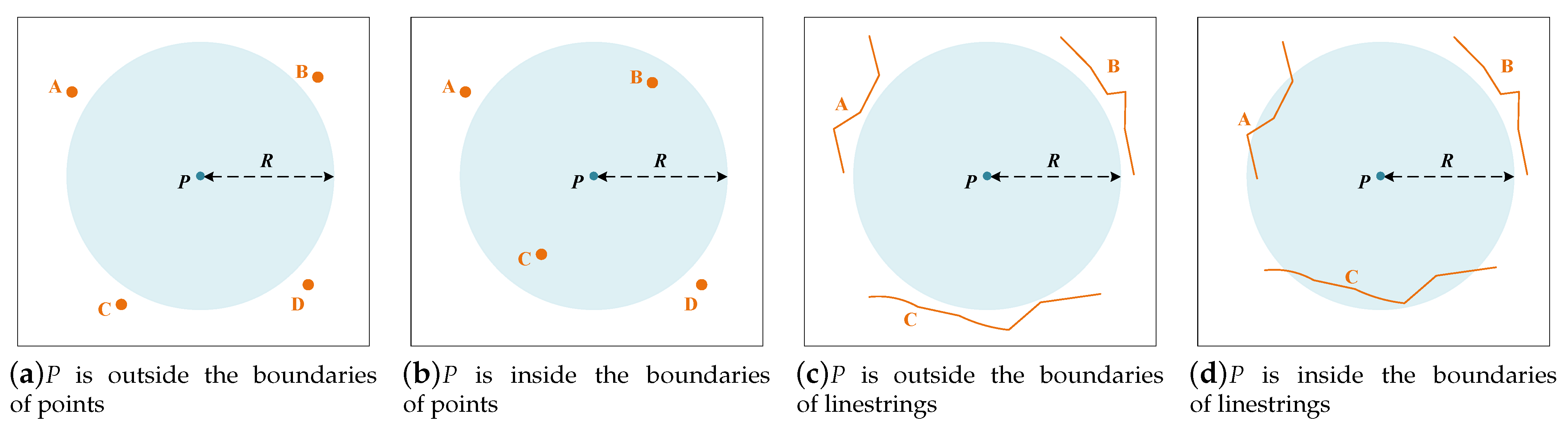
In DisDC, the computing units are pixels rather than spatial objects. In the visualization of vector data based on DisDC, the ultimate goal is to generate a screen display of the vector data, i.e., to generate the pixel values for the screen display, and the key to generating pixel values is to determine whether the spatial location of a pixel is within a certain pixel width of the boundary of vector objects. As shown in Figure 1, given the pixel width R, the problem in determining whether a pixel P is within the spatial range of vector objects with the radius R, can be abstracted as determining whether the circle centered at P with the radius R intersects any vector object. We conclude two features in the processing flow for calculating the pixel values:

• Since the pixels are discrete and regularly distributed, the circle used for intersection judgment is also regular when calculating the value of the pixel P, it must be centered on P with R as the radius to make the judgment.
• Since we only need to generate pixel values for the screen display, we do not need to generate substantial data results in the pixel value generation process, we just need to determine whether any vector objects intersect the circle to generate pixel values.

The process of the visualization of vector data based on DisDC can be divided into two steps: in the first step, to accommodate the above characteristics of spatial relationship determination, pre-processing of the vector data is required. In our previous work, the intuitive approach is to construct a spatial index structure based on the spatial indexing technique described in Section 2.2; in the second step, an efficient spatial range search is used to retrieve the vector objects that intersect the circle, so that the pixel values are generated indirectly from the search results. However, it is difficult to achieve efficient retrieval of large-scale vector data. Firstly, index construction can be very time-consuming, secondly, the index structure retains the vector data and the size of the index inevitably becomes larger as the size of the vector data increases. In HiVision, a current visualization method based on DisDC, the vector data are organized based on the R-tree index structure, which leads to long data pre-processing time and large index occupation while dealing with large-scale geographic vector data.

2.2. Spatial Indexing Methods

Spatial indexing methods are widely used in the retrieval of vector data. It refers to a data structure that is arranged in a certain order according to the position and shape of spatial objects or a certain spatial relationship between spatial objects, which acts as a bridge between the algorithm and spatial objects [21]. The current research on spatial indexing methods can be divided into two categories: the first is the improvement, combination, and variation of traditional spatial indexing methods, and the second is the construction of distributed index by using distributed technologies.

The traditional spatial indexing methods are the grid index, the quadtree index, and the R-tree index. The grid index divides the region into equal or unequal grids and records the spatial objects contained in each grid [4]. The quadtree index is a tree structure that recursively divides geographic space into different levels [22], the nodes in the quadtree have no overlap in space, each node has a specific spatial range, and all vector objects are stored in the leaf nodes. In the construction process, the quadtree has good efficiency: there is initially only one root node, the index range of the root node is usually the minimum bounding rectangle (MBR) of the vector data, which is recursively divided into four equal sub-regions by inserting vector objects until the tree reaches a certain depth or meets a set requirement. The R-tree index is the most commonly used spatial indexing technology at present [23], because it is a highly balanced tree with all leaf nodes at the same level, each vector object is approximated by the MBR which is stored in leaf nodes. The core idea of the R-tree is to gather adjacent nodes together to form a higher-level node which represents the MBR of these nodes until all nodes form a root node. In the construction process, operations such as node splitting and redistribution of child nodes are involved when inserting data to a balanced tree structure, and the dynamic adjustment process is very time-consuming.

The spatial range retrieval process is the same for the quadtree and the R-tree: it needs to determine which child node’s index range intersects with the retrieval range from the root node down, and the search goes deep into the child node to continue, the final retrieval results are obtained after the judgments of leaf nodes are completed. As the growth of the data scale: in the quadtree, limiting the number of layers will result in some leaf nodes storing too many vector objects; limiting the amount of data in the leaf nodes will result in a deeper layer and a more complex structure, both of which significantly affect the retrieval efficiency. The R-tree generally provides better search performance, however, the index range of nodes can overlap, the final results may be obtained after searching multiple paths, the retrieval performance degrades dramatically as the data grows because of the increase of the overlapping area. To solve the problem, current research designs the R-tree variants to improve the performance of R-tree, which can be divided into changes to processes [24,25,26], mixed variation [27], and structural expansion [28,29]. At the same time, the union of the grid index, the quadtree index, and the R-tree index are all realized [30,31,32,33].

With the development of distributed computing technology, distributed index construction, fast query, and high-performance spatial analysis of large-scale vector data on distributed platforms such as Hadoop and Spark have been studied. By comparing the Hadoop platform and MapReduce programming model, Afsin Akdogan et al. concluded that compared with the R-tree index, the spatial index designed by the Voronoi diagram greatly improved the efficiency of query retrieval [34]. Shoji Nishimura et al. proposed a scalable multidimensional data storage scheme MD-HBase and built a Geohash index combining KD-tree and quadtree based on linearization design [35]. Feng Jun et al. proposed a spatial index of HQ-tree based on Hadoop. PR-Quadtree is used in HQ-Tree to solve the problem of low parallel efficiency caused by data insertion sequence and space overlap [13]. LocationSpark [36] is another spatial data warehousing system in Spark environment to support a variety of indexing schemas. A-tree is proposed to optimize a distributed index in cloud computing environments [37]. L. Wang et al. designed a vector spatial data model based on HBase and proposed a parallel method of building Hilbert R-tree index using MapReduce and packed Hilbert R-tree algorithm [38]. S. Huang et al. proposed a multi-version R-tree based on HBase to support multiple concurrent access, which has good scalability and has much higher update throughput and the same level query throughput compared to the original R-tree on HBase [39]. All the methods have improved the retrieval ability of vector data. However, a distributed index mainly focuses on improving the efficiency of data retrieval, without considering the efficiency of index construction and index size: increasing the communication protocol between the cluster nodes causes the index structure to become more complex, and one must fully consider the way of data organization and protocol transmission in the distributed system framework, so index construction costs increase.

In summary, the existing spatial indexing methods are oriented towards data retrieval, data pre-processing efficiency is not a major concern and there are different application scenarios for different index structures. With the growth of data scale, the performance of traditional spatial index has declined sharply, and the adopted distributed technology only focuses on improving the retrieval ability, applying it directly to the visualization process can not achieve high efficiency in data pre-processing and pixel value calculation, and increase the index memory occupation at the same time.

3. Materials and Methods

In this section, the key ideas for vector data pre-processing and visualization in HiIndex are introduced. In the process of vector data visualization based on DisDC, we rasterize vector data and render the final raster images for display, visualization results are organized by the tile pyramid method. As shown in Figure 2, we regard each pixel of the final tile as an independent unit, HiIndex can support vector data pre-processing and pixel value generation for the process.

In HiIndex, firstly, we design an efficient TQ-tree spatial index structure, which is specific to the computational characteristics of vector data visualization based on DisDC. Secondly, the TQ-tree generation algorithm (TQTG) is proposed to quickly construct a TQ-tree based on vector point, linestring, and polygon data, which can improve the data pre-processing efficiency. Finally, based on the computational feature of pixel generation in Section 2.1, we design the TQ-tree-based visualization algorithm (TQTBV) based on the constructed TQ-tree index, TQTBV only needs to judge whether the node in TQ-tree exists to generate pixel values, to achieve fast visualization of large-scale vector data. Compared with the existing visualization method based on DisDC (HiVision) and traditional methods (HadoopViz, GeoSparkViz, and Mapnik), HiIndex significantly improves the efficiency of data pre-processing and visualization. To support real-time visualization of large-scale geographic data, parallel computing technologies are used to accelerate computation, and we extend the high-performance parallel processing architecture in HiVision [15].

3.1. TQ-Tree Spatial Index Structure

To support the visualization of vector data based on DisDC, the core tasks in HiIndex are as follows: (1) the first is to reduce the data pre-processing time; (2) the second is to realize the rapid generation of pixel values. The key to HiIndex is to determine whether a circle centered on the pixel intersects any vector object. According to Section 2.1, the circle must be a regular circle with the pixel as the center and a set pixel distance as the radius, and we just need to determine if any vector objects intersect the circle.

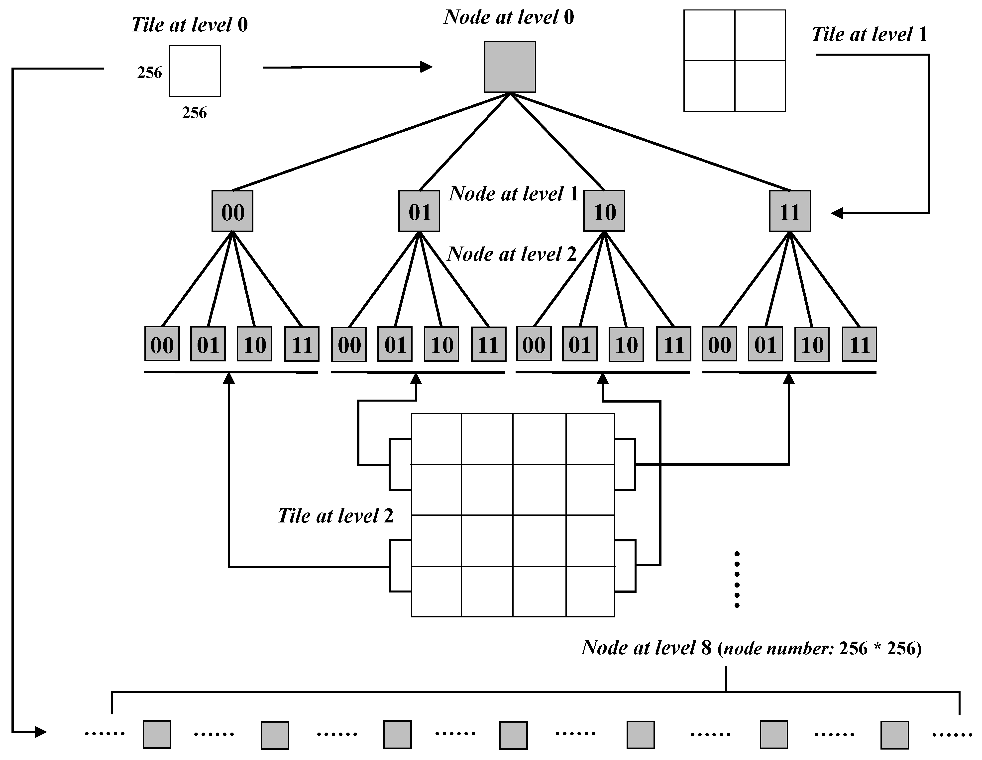
In our research, we analyze if the pixels in the circle can be traversed, if there exists any pixel whose spatial range intersects vector objects, the circle must intersect vector objects. Because the pixels in the circle can be easily calculated from the center pixel and resolution, the difficulty is to determine whether the spatial range of a pixel intersects with any vector objects. In the tile pyramid, the specification of each tile is 256 × 256 pixels, each tile and each pixel in the tile have a unique geographic spatial range, if an index structure is designed where the index range of nodes is relatively equal to the spatial range of pixels, multiple judgment paths will not be generated during judgment and the judgment speed will be improved.

Based on the above considerations, we improve the quadtree and design the TQ-tree structure in HiIndex. As shown in Figure 3, TQ-tree takes the node as the minimum storage unit and the node is divided into five types: root node, left-bottom node, right-bottom node, right-upper node, and left-upper node. There is only one root node in the TQ-tree. In each node, attribute information such as coding, spatial range, node type, child node pointers, and parent node pointer is recorded. Parent-child nodes are connected by pointers, and the pointer is null when the child node or parent node does not exist. When TQ-tree is full, the number of nodes at each level is shown in Equation (1), where i denotes the i-th level in TQ-tree:

$$NodeNumbe{r}_i=2^i\times 2^i$$

(1)

When setting the node’s spatial range, which is different from the MBR of a dataset, which is set as the index range of the root node in a quadtree, the global spatial range under the spherical Mercator projection is taken as the index range of the root node whatever the dataset is. Then the index range of the root node is recursively quartered and set as the spatial range of its child nodes. At the same time, the encoding properties of the child nodes are set. Geohash is a common address encoding method that encodes two-dimensional spatial location data into a binary string [40]. In HiIndex, the Geohash method is used to recursively divide the global spatial range under spherical Mercator projection. As shown in Figure 4, from the root node to code down: for each recursion to the next level, set “00” as the code of the left-bottom node, “01” as the code of the left-upper node, “10” as the code of the right-bottom node, and “11” as the code of the right-upper node. Thus, each node in TQ-tree is guaranteed to have a unique number, and the inclusion relationship of parent-child nodes in the spatial range is reflected through encoding.

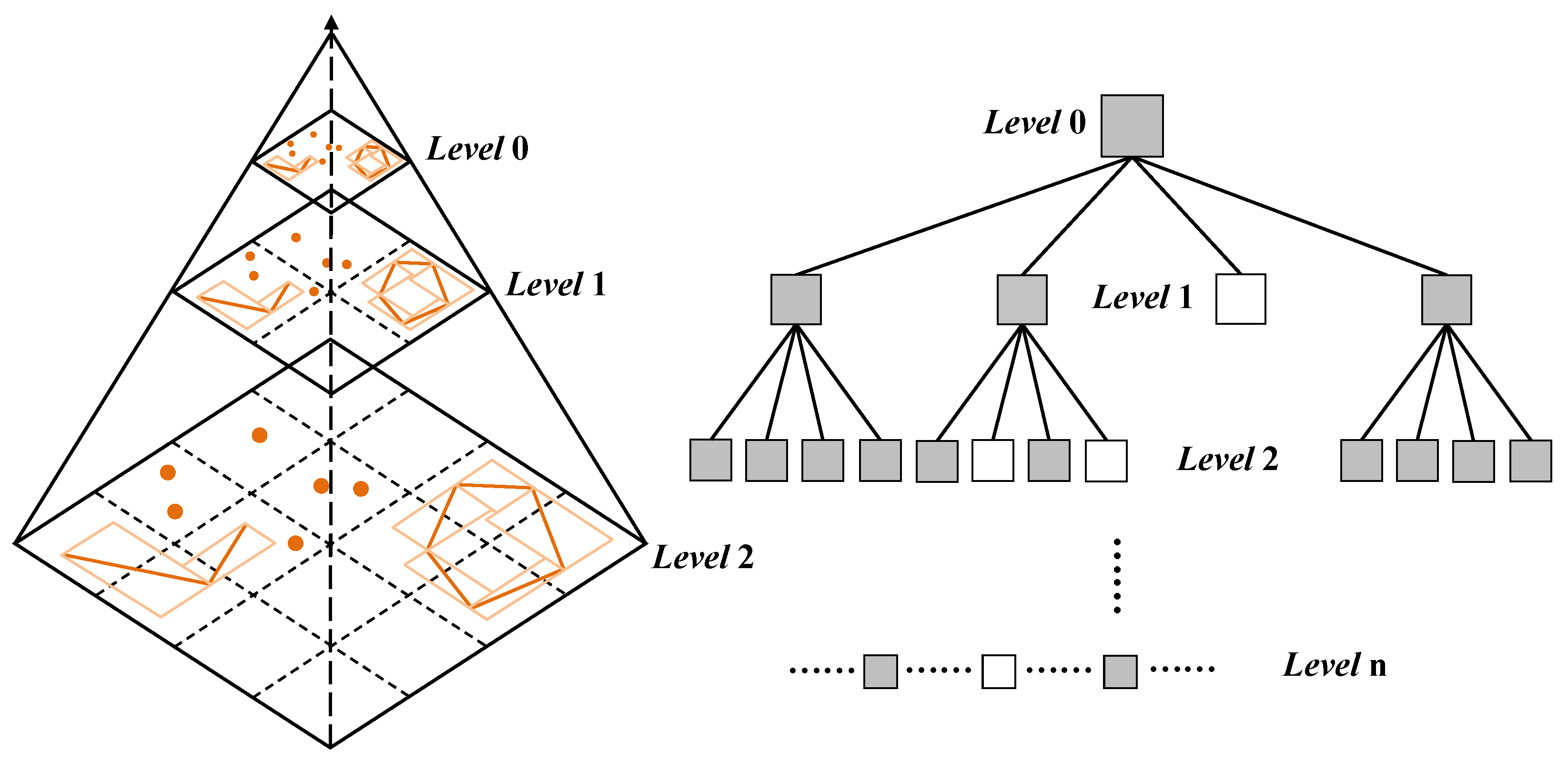
The nodes in the TQ-tree have two features: firstly, the index range of nodes of level n in the TQ-tree are consistent with the spatial range of tiles of level n in the tile pyramid. In Figure 5, the index ranges of the four nodes of level 1 in the TQ-tree are the same as those of the four tiles of level 1 in the tile pyramid. Secondly, since the tile size is regular 256 × 256 pixels, the spatial range of pixels of a tile can be considered to be obtained by recursively dividing the spatial range of the tile for eight times, which is consistent with the index range of 256 × 256 child nodes obtained after eight recursive quarts of the node corresponding to the tile in the TQ-tree. Therefore, starting from level 8 in the TQ-tree, the index range of nodes of level n not only has the first feature but also is consistent with those of pixel of the tile of level $n-8$ in the tile pyramid. In Figure 5, after eight recursive quarts of the index range of the root node, 256 × 256 child nodes are obtained at level 8 of the TQ-tree, and the index ranges of these child nodes are aligned with the spatial range of 256 × 256 pixels of the tile corresponding to the root node.

The design of the TQ-tree structure can realize efficient data pre-processing and rapid visualization of large-scale vector data. Firstly, compared with the R-tree indexing techniques, the data insertion during the quadtree index construction has little effect on the construction speed. Secondly, if the node is created only when it intersects any vector object, the problem of determining whether the spatial range of a pixel intersects any vector object can be converted to the issue of whether the node exists or not, this is based on the characteristics of nodes. When the spatial range of a pixel is taken as the retrieval range, the retrieval range will not intersect with the node index range, so there will be no multiple judgment paths. By coding the spatial range of the tiles/pixels, the corresponding node can be quickly located by the unique encoding of a tile/pixel, which can be achieved by simple string manipulation with minimal computational complexity.

3.2. TQTG for Point, Linestring, and Polygon Edges

In the index construction stage, TQTG adopts the recursive division method to construct a TQ-tree in the “top-down” way. A root node is created firstly, and then new child nodes are created based on whether the vector object intersects the recursively divided spatial range of the root node. In TQTG, vector objects are divided into small fragments [15]: for point objects, a point object is directly used as a fine-grained item; for line objects, the MBR of each line segment is taken as a fine-grained item; for polygon objects, take the MBR of each edge as a fine-grained item. The details of TQTG for point are shown in Algorithm 1, the details of TQTG for linestring or polygon edges are shown in Algorithm 2. TQTG is mainly divided into three steps:

• Step 1: Create the initial root node ($rNode$) based on the function (NODE) which set the global spatial range ($R_{global}$) as the index range of the root node whatever the dataset is, the parent node ($pNode$) and the child node pointer ($cNodes$) are null. At the same time, set the maximum level ($maxLevel$) of the TQ-tree.
• Step 2: Iterate through the vector objects in the dataset, recursively creating new nodes by inserting fine-grained items of vector objects one by one.

  -

  For point objects (P): Traverse the point object (p), with intermediate variables (R, $tNode$) whose initial values are set to $R_{global}$ and $rNode$ for recursive judgments. Divide R equally into four quadrants ($r_{lb},r_{lu},r_{rb},r_{ru}$) by the function (DIVIDE), create a child node ($lbNode$/$luNode$/$rbNode$/$ruNode$) with $r_{lb}/r_{lu}/r_{rb}/r_{ru}$ as the node index range when $r_{lb}/r_{lu}/r_{rb}/r_{ru}$ contains p, point the child nodes pointer ($tNode.cNodes[lb/lu/rb/ru]$) to the newly created node, and set $r_{lb}/r_{lu}/r_{rb}/r_{ru}$ and $lbNode$/$luNode$/$rbNode$/$ruNode$ as the values of R and $tNode$. In this way, judge recursively until the level of the newly created node ($tNode.level$) is no higher than $maxLevel$.

  -

  For line/polygon objects (L): Traverse the line/polygon object (l): firstly, the MBR of a line/polygon object ($l.MBR$) is obtained, and the smallest node containing the MBR ($tNode$) is created recursively from $rNode$ by the function (MCNODE). Secondly, each fine-grained item (s) of l is inserted one by one from $tNode$ to create nodes by the function (InsertSegment), which is the same as the process of inserting a point object, the difference is that the child node ($lbNode$/$luNode$/$rbNode$/$ruNode$) is created when $r_{lb}/r_{lu}/r_{rb}/r_{ru}$ intersects s. When more than one of the four ranges intersects s, recursive judgment on the intersection range one by one is required.

• Step 3: When all items are inserted, the root node and new nodes form a TQ-tree, which can support the rendering of tiles at level 0 − (n− 8) of the tile pyramid, and the attribute information of all nodes is stored line by line as a binary file in the external disk storage.

Figure 6 shows the constructed TQ-tree of a dataset, the TQ-tree is a non-full quadtree structure, which does not cause memory wastes. At the same time, each node in the tree has a specific meaning: when a node exists, the spatial range of the node must intersect with vector objects. For example, there is no spatial object in the spatial range of the tile in the right-bottom corner of level 1 in the tile pyramid, then the corresponding node of level 1 in the TQ-tree does not exist.

Algorithm 1: TQ-tree generation for point.

Algorithm 2: TQ-tree generation for linestring/polygon edges.

3.3. TQTBV for Point, Linestring, and Polygon Edges

From Section 2.1 and Figure 1, in the visualization of vector data based on DisDC, the core task is determining whether the circle centered at a pixel P intersects any vector object, and the judgment only focuses on “yes or no”. To achieve the determination of the above relationship, TQTBV is designed based on the constructed TQ-tree index.

In TQTBV, the key of the task is determining whether the spatial range of a pixel in the circle intersects any vector object. In the constructed TQ-tree: firstly, since the spatial range of tiles/pixels is aligned with the index range of nodes, there will not be multiple judgment paths when judging with the spatial range of a pixel, and we can directly locate the node by encoding the tile/pixel to be computed and performing a simple string operation on the Geohash encoding; secondly, if the node exists, it means that the spatial range of the tile/pixel corresponding to the node intersects vector objects. Thus, the discrimination issue can be transformed into the issue of judging whether the node exists in the TQ-tree.

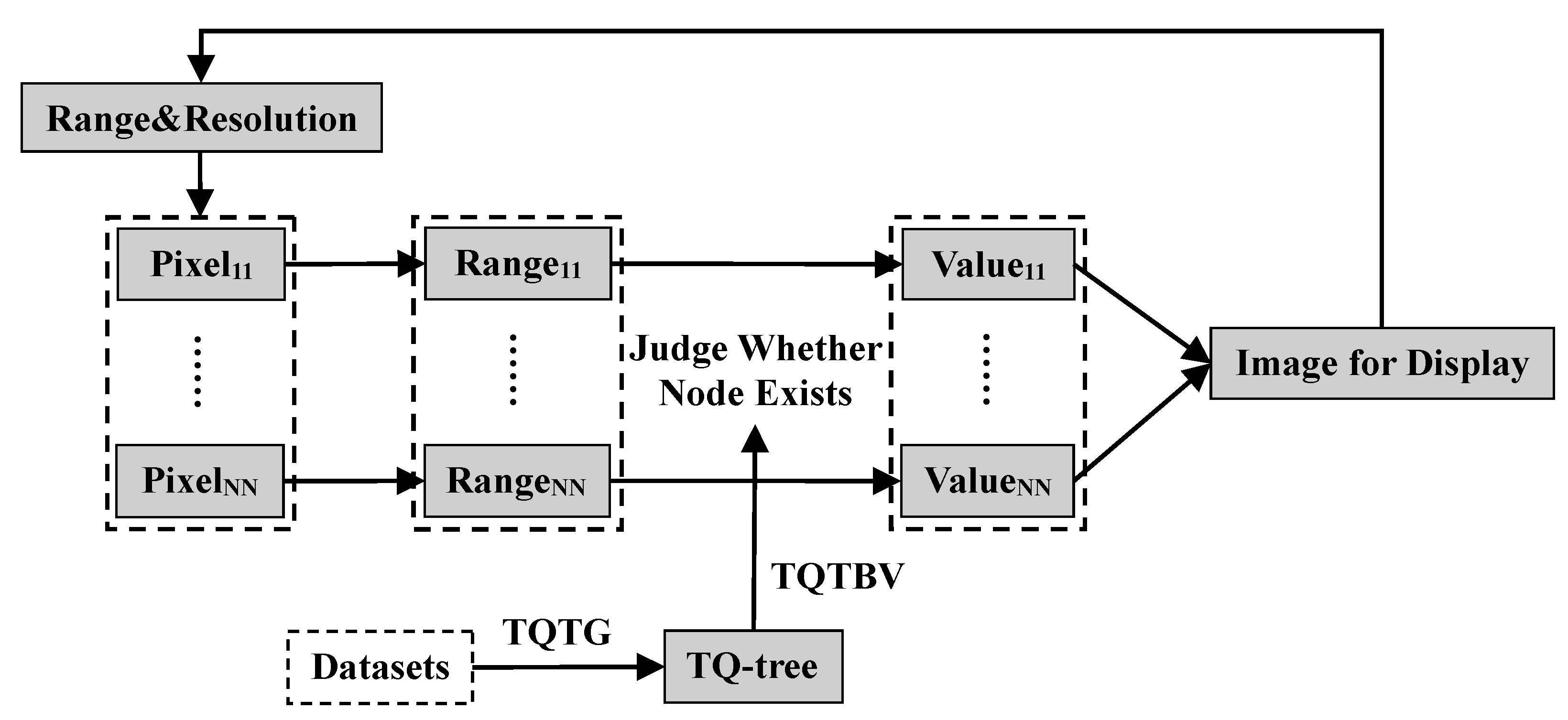
The details of TQTBV are shown in Algorithm 3. In TQTBV, we visualize point, line, and polygon objects in a set pixel width (R). To generate the value of the pixel (P) in the tile (T). TQTBV is mainly divided into three steps:

• Step 1: It is first determined whether the tile (T) needs to be drawn. The encoding ($tileNode$) of the tile is obtained by the tile level (L) based on the function (GEOHASH), and the corresponding node ($tileNode$) is searched from the constructed TQ-tree ($TQtree$) by the function (FIND). If $tileNode$ is empty, the value of P is set to 0 and the tile does not need to be drawn. Otherwise, the pixel value is calculated in the following steps.
• Step 2: The value of P is calculated by determining whether there is any pixel in the circle whose corresponding node exists in the TQ-tree. Since P is undoubtedly inside the circle, the encoding ($pixelCode$) of P is obtained by the pixel level ($L+8$), and the corresponding node ($pNode$) is searched from $tNode$. If $pNode$ is not empty, the value of P is set to 1. Otherwise, the pixel value is calculated in Step 3.
• Step 3: The pixel resolution ($R_z$) and the minimum level n containing the circle are computed. Since the pixel closer to P is more likely to be in the circle, we calculate the pixels ($NP$) from inside to outside, that is, from pixels in level 1 to pixels in level n. If the distance between a pixel ($np$) in $NP$ and P is less than R, the encoding ($npCode$) of $np$ is obtained and the corresponding node ($npNode$) is also searched from $tNode$, If $npNode$ is not empty, the value of P is set to 1. Otherwise, the value of P is set to 0.

TQTBV has two advantages: firstly, it determines whether the tile is drawn by prejudging whether the corresponding node exists, which can reduce the rendering of blank tiles. Secondly, it converts the spatial topology discrimination issue to the problem of whether the node exists, which can be determined quickly through encoding, it greatly reduces the time of spatial intersection judgment and the rendering time of each tile.

Algorithm 3: TQ-tree-based visualization.

4. Experiment

In this section, we conduct several experiments to evaluate the high performance of HiIndex. By comparing with HiVision and traditional methods such as HadoopViz, GeoSparkViz, and Mapnik, the advantages of HiIndex in index construction time, memory occupation, and tile rendering speed are verified. Firstly, we compare the index construction time of HiIndex and HiVision to verify the advantages of HiIndex in the stage of data pre-processing. Then, we compare the index occupation generated by HiIndex and HiVision, and verify the advantages of HiIndex in output index to external memory. Moreover, we test the tile number required rendering and tile rendering speed of HiIndex, HiVision, and traditional methods, and verify the advantages of HiIndex in real-time interactive visualization of supporting large-scale geographic vector data. Finally, to evaluate the applicability of HiIndex, the index construction time and index size are calculated when building TQ-tree of different layers in HiIndex.

All the experiments are conducted on a cluster with four nodes (

Table 1. Experimental environment.

Item	Description
CPU	4 × 32 cores, Inter(R) Xeon(R) [email protected] GHz
Memory	4 × 512  GB
Operating system	Centos7.1

). The computer node of HiIndex is implemented in c++, based on c++ 1.64, MPICH 3.2, Redis 3.2.12, Hicore 1.0 which is an efficient library for reading vector data. The HiVision is based on the same library as above.

Table 2. Datasets used in the experiments.

Dataset	Type	Records	Size
${\mathrm{L}}_1$: OSM postal code areas boundaries	linestring	210,054	65,334,342 segments
${\mathrm{L}}_2$: OSM boundaries of cemetery areas	linestring	193,339	1,800,980 segments
${\mathrm{L}}_3$: OSM sporting areas boundaries	linestring	1,783,952	18,969,047 segments
${\mathrm{L}}_4$: OSM water areas boundaries	linestring	9,211,000	376,208,235 segments
${\mathrm{L}}_5$: OSM parks green areas boundaries	linestring	11,634,551	396,527,008 segments
${\mathrm{L}}_6$: OSM roads and streets	linestring	72,336,396	717,048,198 segments
${\mathrm{L}}_7$: OSM all linestrings on the planet	linestring	106,268,554	1,573,469,984 segments
${\mathrm{P}}_1$: OpenCeilliD cell tower locations	point	40,719,478	40,719,478 points
${\mathrm{P}}_2$: OSM all points on the planet	point	2,682,401,763	2,682,401,763 points
${\mathrm{A}}_1$: OSM buildings	polygon	114,839,692	804,028,282 edges
${\mathrm{A}}_2$: OSM all polygons on the planet	polygon	181,772,692	2,077,524,465 edges

shows the datasets used in the experiments, and the datasets are all on the planet level including points, linestrings, and polygons data. ${\mathrm{P}}_1$ is from OpenCellID, which is the world’s largest collaborative community project that collects the positions of GPS base stations. Other datasets are from OpenStreetMap, which is an editable online mapping service built through crowdsourced volunteered geographic information. ${\mathrm{L}}_7$, ${\mathrm{P}}_2$, and ${\mathrm{A}}_2$ respectively contain all the linestrings, points, and polygons data on the planet from OpenStreetMap, there are more than 1 billion segment/point/edge items in each of the dataset. In the experiments, the same data source is used for each of the visualization tools.

4.1. Experiment 1. Comparison of Data Pre-Processing Efficiency

In this experiment, to verify the high efficiency of HiIndex in data pre-processing, HiIndex and HiVision are compared and analyzed. Both algorithms are implemented in the given experimental environment. In HiVision, vector data are organized by constructing R-tree spatial indexes based on a quadratic algorithm, which enables rapid index establishment [41]. In HiIndex, a TQ-tree of 17 layers is constructed by TQTG. The spatial indexes generated by the two algorithms are output to external storage.

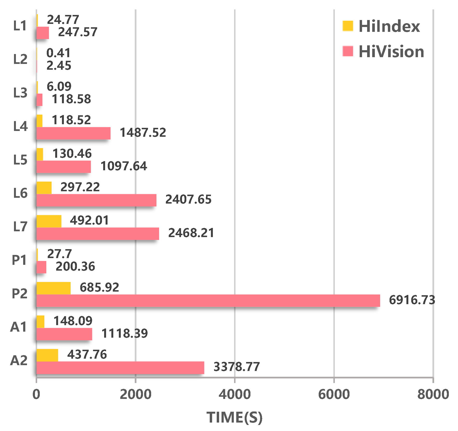
Figure 7 shows the comparison of the index construction time of the two methods. The results show that firstly, for each dataset, HiIndex’s index construction rate is much higher than that of HiVision, the minimum construction efficiency of two methods is 5 times (=2468.21 s ÷ 492.01 s) on ${\mathrm{L}}_7$, and the maximum is 19 times (=118.58 s ÷ 6.09 s) on ${\mathrm{L}}_4$. Secondly, for 100 million-scale datasets (${\mathrm{L}}_{4-7}$, ${\mathrm{P}}_2$, ${\mathrm{A}}_{1-2}$), it takes a long time to build indexes by HiVision. This is because the R-tree construction process is a dynamic process of constant adjustment, and the data in nodes and even the whole R-tree hierarchy need to be adjusted again. Therefore, index construction is very time-consuming. The index construction time of HiIndex is much shorter than that of HiVision. For the billion-scale datasets ${\mathrm{L}}_7$, ${\mathrm{P}}_2$, and ${\mathrm{A}}_2$, the index construction time of HiIndex is only 19.94% (=492.01 s ÷ 2468.21 s), 9.92% (685.92 s ÷ 6916.73 s), and 12.96% (437.76 s ÷ 3378.77 s) of HiVision respectively.

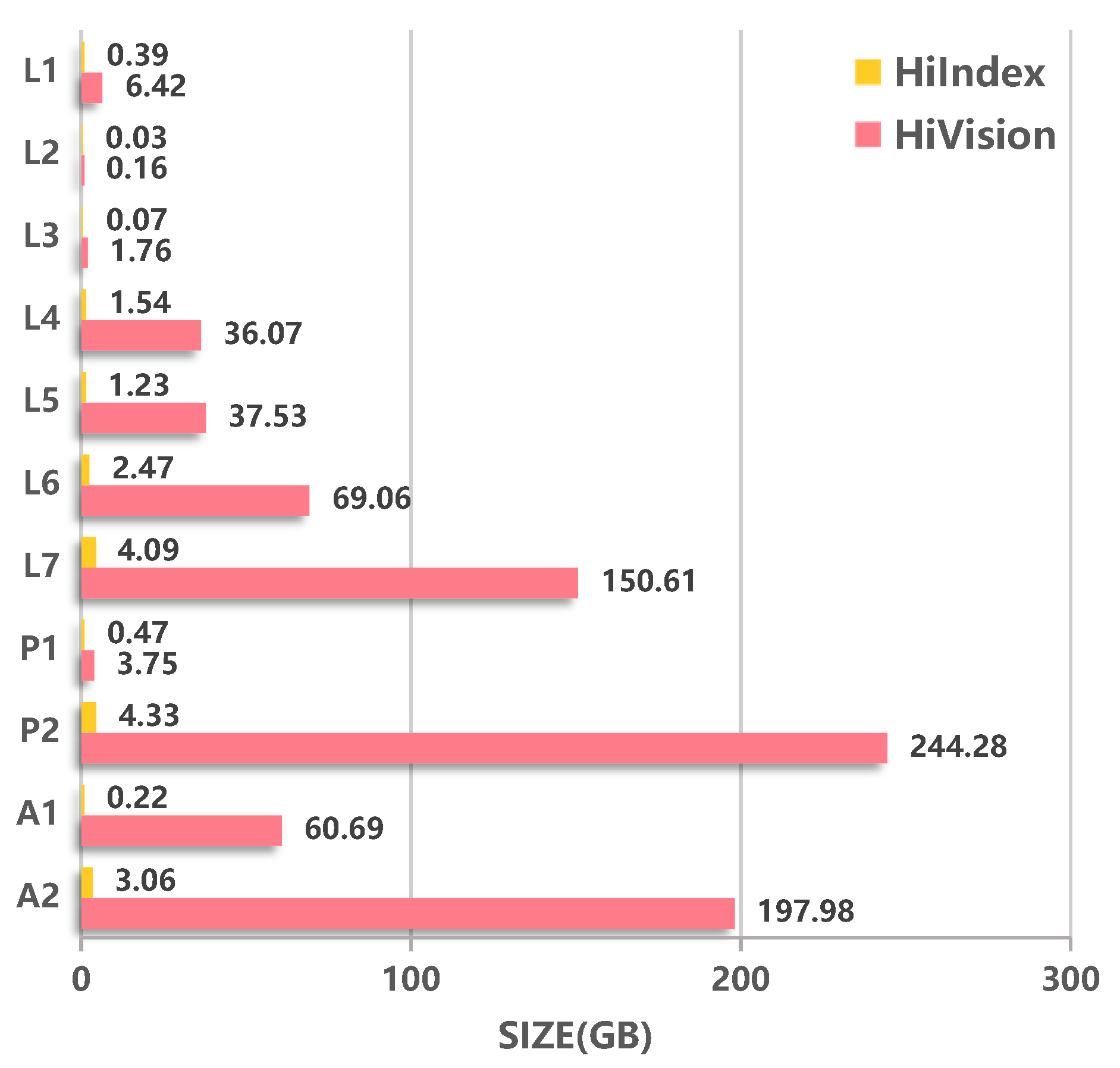
Figure 8 compares the occupation of the output index of the two methods in disk storage. From the experimental results, the index occupation of HiIndex is much smaller than that of HiVision. For the billion-scale datasets ${\mathrm{L}}_7$, ${\mathrm{P}}_2$, and ${\mathrm{A}}_2$, the index size is only 2.72% (=4.09 GB ÷ 150.61 GB), 1.77% (=4.33 GB ÷ 244.28 GB), and 1.55% (=3.06 GB ÷ 197.98 GB) of HiVision respectively. The reason is that TQTG only needs to store TQ-tree node information, thus saving a lot of storage space.

To sum up, in terms of data pre-processing for large-scale geographic vector data, HiIndex has a shorter index construction time and smaller memory occupation, which has an excellent performance.

4.2. Experiment 2. Comparison of Visualization Efficiency

In the previous work, we compared HiVision with three typical data-driven methods (e.g., HadoopViz, GeoSparkViz, Mapnik), and verify HiVision produces higher performance with better visualization effects [15], which proves that the method based on DisDC has better performance than traditional data-driven methods. HiIndex, like HiVision, is also a method based on DisDC, and the experiment mainly verifies the advantages of HiIndex in visualization efficiency compared to HiVision and traditional methods in the visualization of large-scale vector data. In the cluster environment, we run 128 MPI processes and 2 OpenMP threads in each process to generate tiles. For each dataset, the two algorithms and three traditional methods are used to generate tile data at levels 1, 3, 5, 7, and 9.

Figure 9 shows the comparison of the total time taken by different methods to generate all tiles of zoom levels 1, 3, 5, 7, and 9. From the figure, HiIndex and HiVision show superior tile rendering performance when dealing with large datasets compared to three traditional approaches, which indicates that the methods based on DisDC have obvious advantages in processing large-scale geographic vector data. At the same time, for all datasets, the time taken by HiIndex to generate tiles is far less than that of HiVision and the three traditional methods. For the billion-scale datasets ${\mathrm{L}}_7$, ${\mathrm{P}}_2$, and ${\mathrm{A}}_2$, the total time of generating all tiles by HiIndex is only 7.62% (=20.47 s ÷ 268.61 s), 4.92% (=19.59 s ÷ 398.32 s), and 4.99% (=29.48 s ÷ 590.62 s) of HiVision, respectively. From ${\mathrm{L}}_1$ to ${\mathrm{L}}_7$, with the increase of dataset size, compared with HiVision, the time consumption of HiIndex to generate all tiles has a small growth trend, indicating that HiIndex is more insensitive to data size. HiIndex is efficient because it requires fewer tiles to render and it is faster to render tiles.

Figure 10 shows the number of tiles required to be rendered by the two algorithms when generating tile data at levels 1, 3, 5, 7, and 9. According to experimental results, for all datasets, the number of tiles required to be rendered in HiIndex is far less than that in HiVision. When taking HiVision to render tiles, it needs to determine whether the tile’s spatial range and the MBR of dataset intersection, when the tile’s spatial range is contained in the MBR of the entire dataset but there is no vector object in the tile’s spatial range, a large number of blank tiles will be drawn, and the more blank tiles will be drawn as the zoom level increases. When taking HiIndex to render tiles, it discriminates and avoids rendering blank tiles.

Figure 11 shows the generation speed of tiles at various levels by using different methods. From experimental results, the data-driven methods show a higher rate of rendering speed at higher levels than HiVision, but HiVision shows an overall high rate of tile generation at each level, especially at lower levels. The rendering speed at level 1 in ${\mathrm{A}}_2$ reached 240.47 tiles/s, the number of tiles within the viewport of the user is usually no more than 50, so HiVision has the capability to support real-time visualization. At the same time, for all datasets, the tile generation speed of HiIndex at all levels is much faster than that of HiVision and three traditional methods, and the smallest rendering speed of HiIndex in ${\mathrm{A}}_2$ reached 944.28 tiles/s, which shows HiIndex has stronger real-time visualization capability.

To sum up, HiIndex has great advantages in large-scale geographic vector data visualization, and it can provide more options for visualization. It can quickly generate tile cache in a short time and support real-time interactive visualization.

4.3. Experment 3. The Applicability of HiIndex

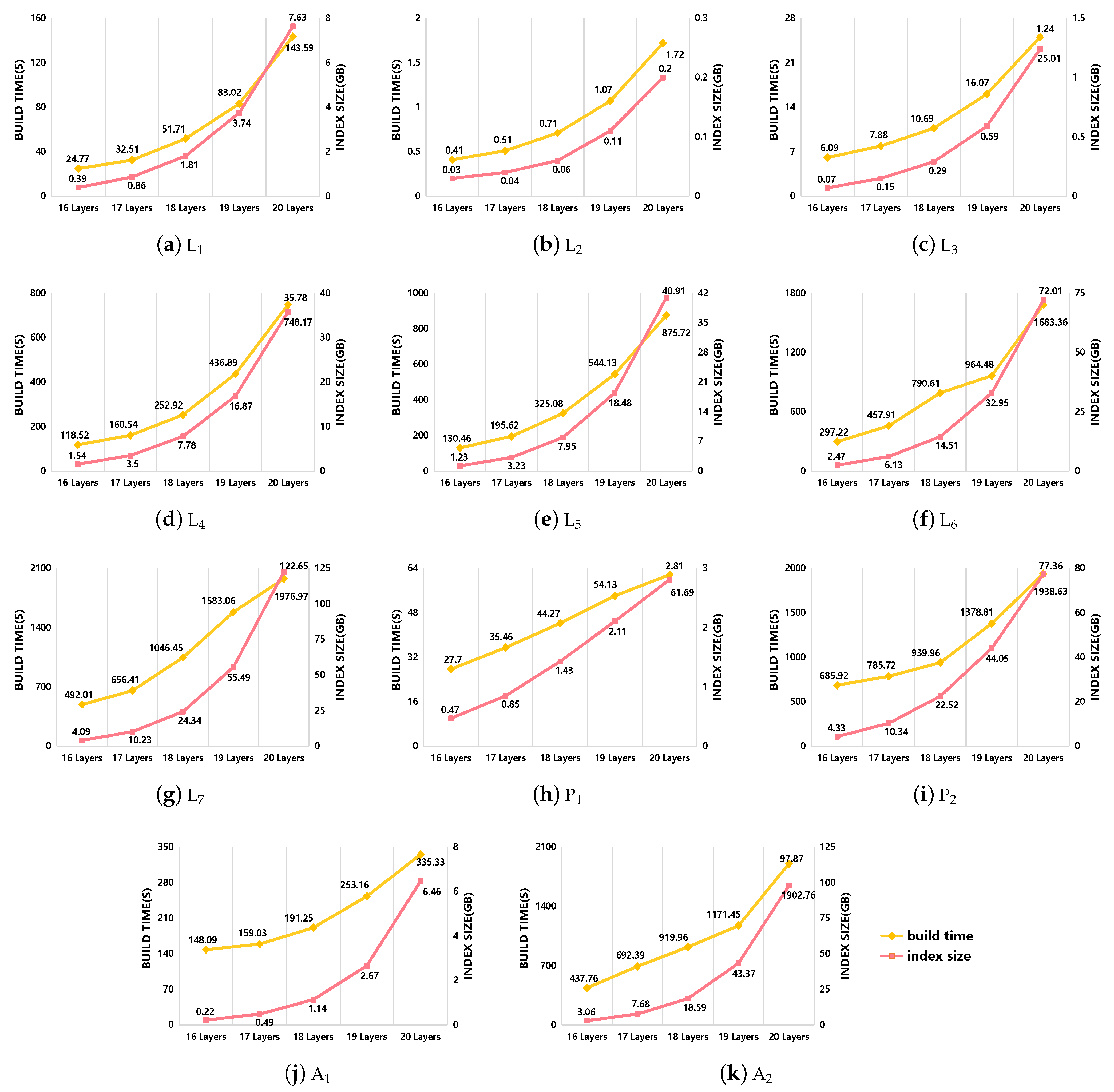
This section mainly verifies the applicability of HiIndex. The performance of HiIndex includes the index construction time and the index occupation, and the main factor affecting its performance is the total layers of the TQ-tree. When the TQ-tree layers increase, the number of recursive judgments increases when inserting vector objects in TQTG, and the index construction time becomes longer. At the same time, the number of nodes in the TQ-tree increases, and the index occupation increases. In HiIndex, we construct a TQ-tree with a total number of layers between 16 and 20 based on different datasets and count the index construction time and index size. The results are shown in Figure 12. For each dataset, the index construction time and index size generally show an exponential growth trend with the increase of the layers, and the growth rate begins to increase when the TQ-tree layers are 18 layers for the billion-scale datasets ${\mathrm{L}}_7$, ${\mathrm{P}}_2$, and ${\mathrm{A}}_2$. Combined with the comparison between Figure 7 and Figure 8, when the total number of TQ-tree layers is 20 layers, the index construction time of HiIndex has reached 80.1% (=1976.97 s ÷ 2468.21 s), 28.0% (=1938.63 s ÷ 6916.73 s), and 56.3% (1902.76 s ÷ 3378.77 s) of HiVision, the index size has reached 81.4% (=122.65 GB ÷ 150.61 GB), 31.7% (=77.36 GB ÷ 244.28 GB), and 49.4% (=97.87 GB ÷ 197.98 GB) of HiVision. As the total layers of TQ-tree increase continually, the advantages of HiIndex are not obvious.

Based on the experimental results and analysis, the following conclusions can be drawn: when using HiIndex to visualize unknown large-scale datasets, HiIndex is best used to visualize data at zoom levels 0–12. At this time, the rapid and real-time visualization requirements of most vector data at the browsing level have been met. In other words, when the maximum browsing level of data is small, we only need to build a TQ-tree with small total layers, and HiIndex has high efficiency. When the maximum browsing level of data is large, the total layers of TQ-tree should not be higher than 20 layers, that is, the maximum browsing level should not be higher than 12 levels.

5. Conclusions and Future Work

In this paper, we propose HiIndex, a data organization method for DisDC, to realize the rapid organization of large-scale vector data and provide a rapid visualization algorithm for DisDC. Different from the traditional method, the TQ-tree structure is designed in HiIndex, and each node in the tree corresponds to a specific and regular spatial range of tile/pixel. In HiIndex, the TQTG algorithm is firstly designed to build TQ-tree to realize the rapid organization of data, and then the visualization algorithm TQTBV is designed based on the constructed TQ-tree, and parallel computing technologies are used to accelerate efficiency, enabling rapid visualization of data. Different experiments are designed and conducted to evaluate the performance of HiIndex, DisDC-based method HiVision and traditional methods. Experiment 1 shows that compared with the existing methods, HiIndex has a higher efficiency in data organization, because its index construction time is shorter and the index occupation is smaller. Experiment 2 proves the advantage of HiIndex in large-scale vector data visualization, which lies in its faster tile rendering speed and fewer tiles needed to be drawn. Experiment 3 tests the applicability of HiIndex. From the experimental results, it can be seen that HiIndex has obvious advantages in achieving data browsing of large-scale data at the 0–12 level, especially at the low levels. Additionally, most of the difficulties and requirements of data visualization are based on low-level data browsing, so HiIndex has met most of the visualization requirements. In this article, we only design the algorithm based on DisDC for rapid visualization of large-scale geographic vector data in HiIndex. In the future work, we will focus on applying HiIndex to other spatial analysis problems such as spatial buffer analysis, spatial overlap analysis, spatial linkage analysis, and designing corresponding DisDC visual analysis algorithms to expand the application fields of HiIndex.