
Estimating the Soil Erosion Cover-Management Factor at the European Part of Russia


Abstract
:1. Introduction
- Thick cover (winter and spring crops, leguminous crops, annual grasses)
- Tilled high-stem (corn, sunflower)
- Tilled low-stem (potatoes, sugar beet)
- Perennial grasses (second-third years of vegetation)
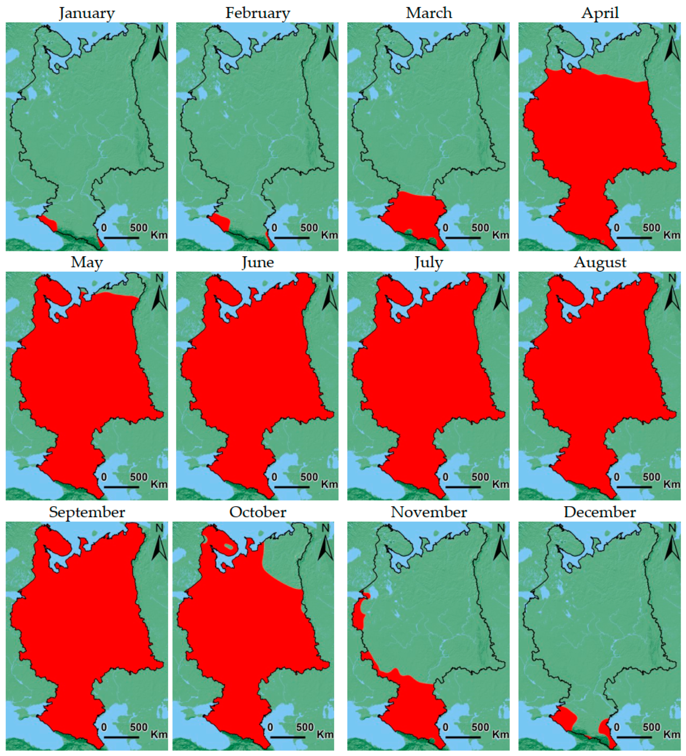
- The seasonality of precipitation has been determined, i.e., areas with rainfalls in a particular month are identified;
- Due to the lack of government statistical and spatial data on the structure of cultivated areas and crop rotation, crop recognition was carried out using data from peer territories (Canada);
- Using free products of biophysical parameters calculated on the basis of remote sensing data, the phenological phases of vegetation were determined;
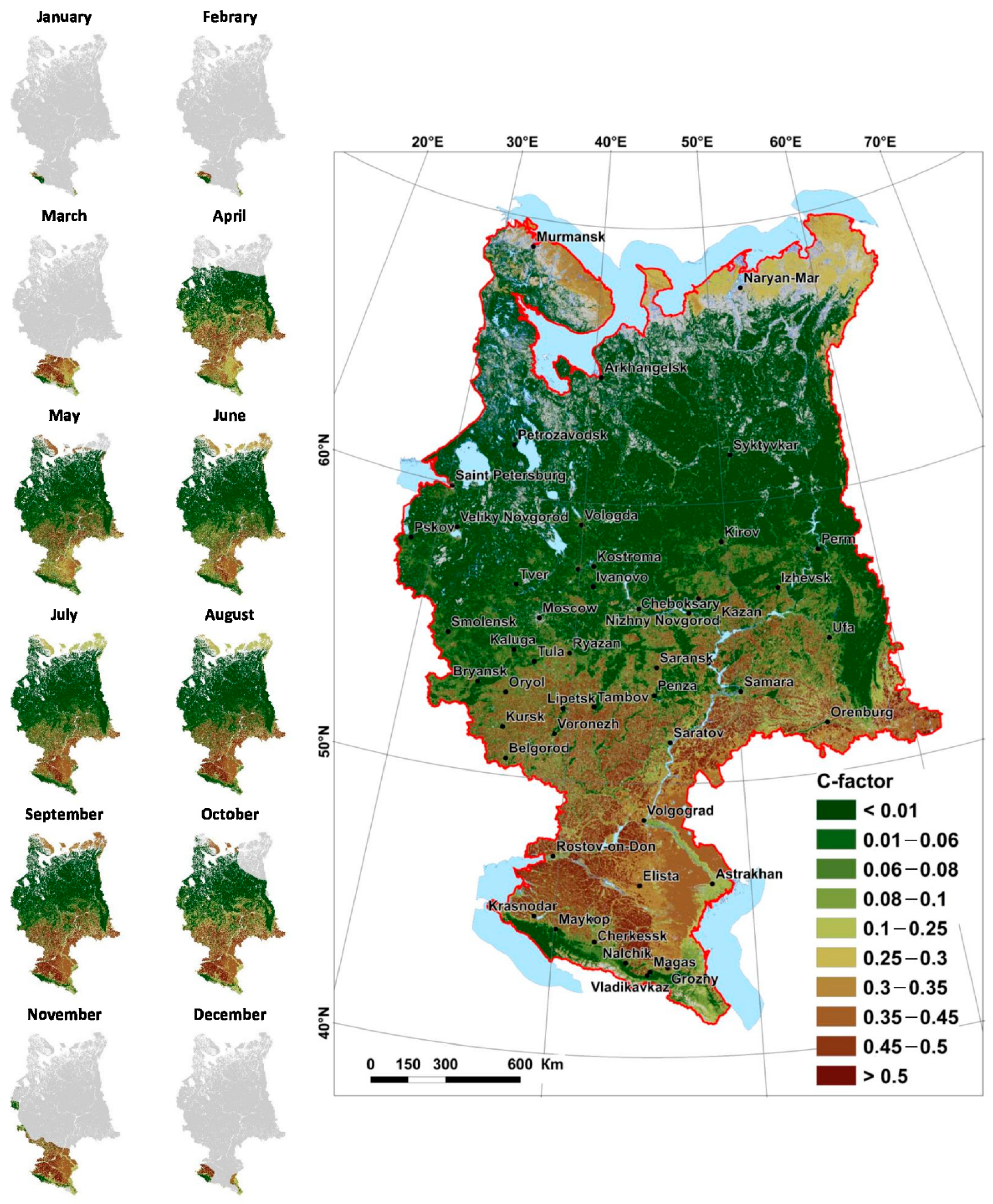
- The annual and monthly mean values of C-factor for the study area were calculated.
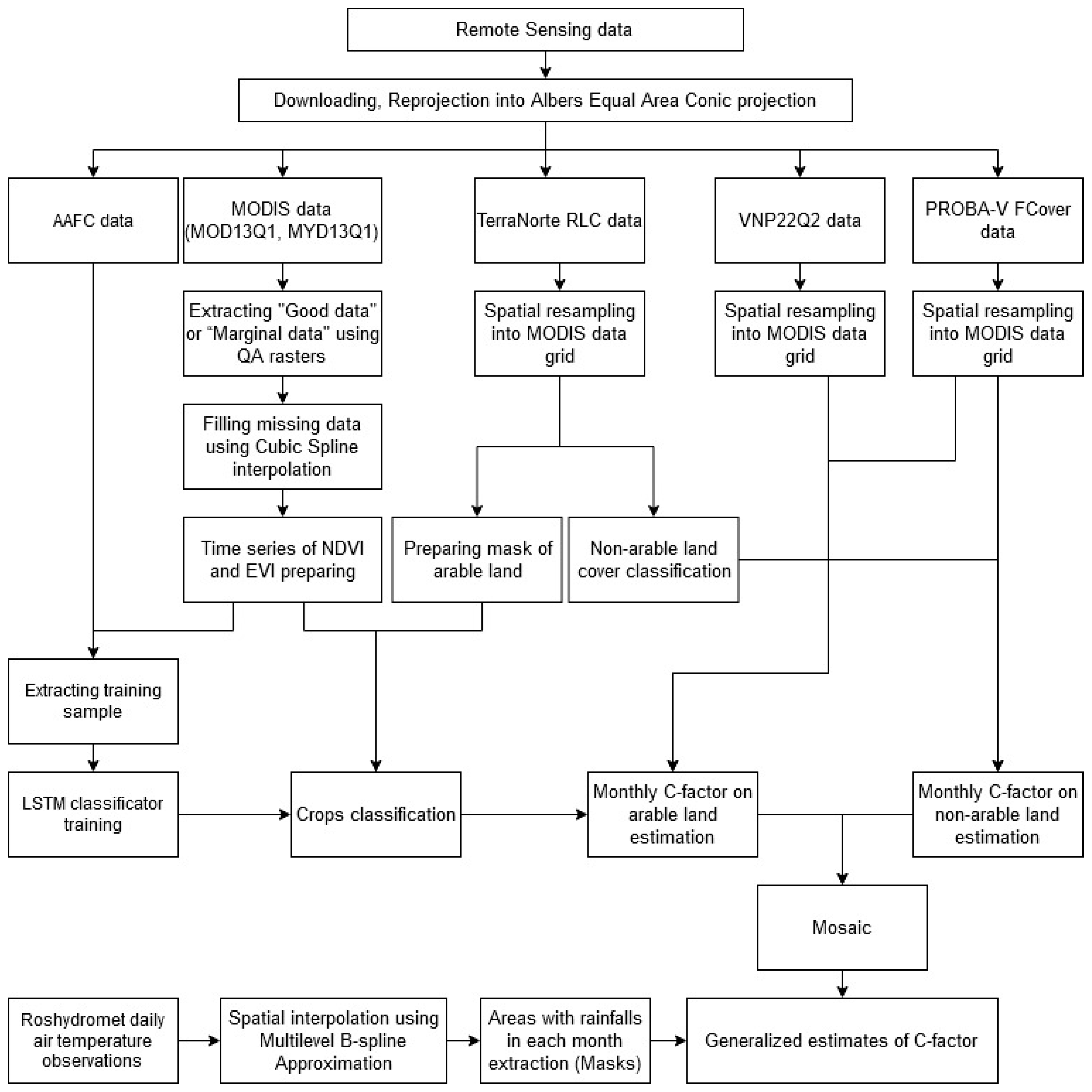
2. Materials and Methods
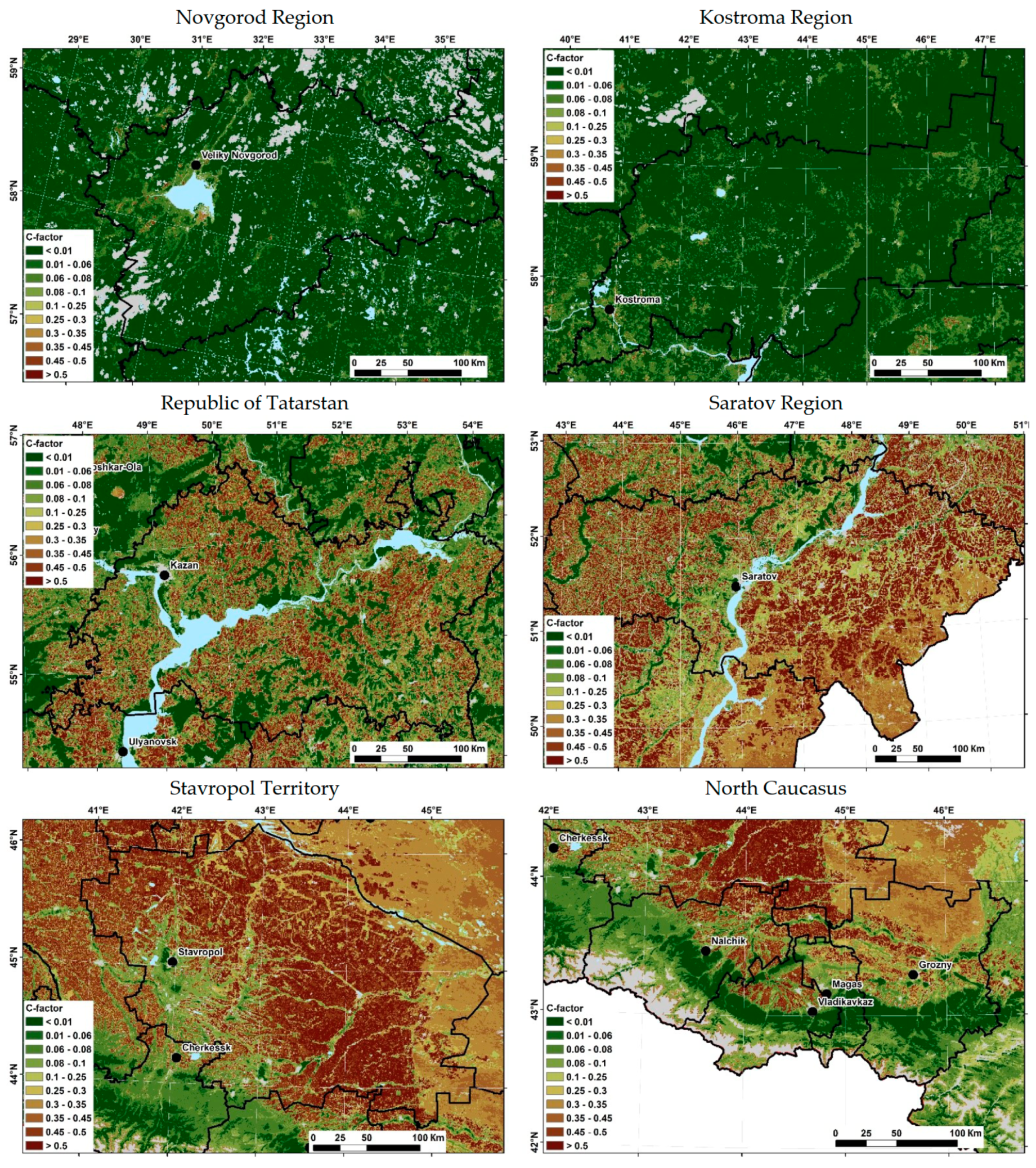
2.1. Study Area
2.2. Input Data
- Products MOD13Q1, MYD13Q1 obtained from the MODIS satellite imagery data from Terra and Aqua satellites-16-day composites of NDVI and EVI vegetation indices with a spatial resolution of 250 m;
- VNP22Q2 products obtained from VIIRS satellite imagery data from the Suomi NPP satellite-annual indicators of the phenology of the land surface with a spatial resolution of 500 m. The product contains six phenological transition dates: onset of greenness increase, the onset of greenness maximum, the onset of greenness decrease, the onset of greenness minimum, dates of mid-green, and senescence phases;
- FCover product obtained from PROBA-V satellite imagery data. 10-day composites of the biophysical parameter FCover-the fraction of the surface covered by any green vegetation type, with a spatial resolution of 300 m.
2.3. C-Factor Assessment Method
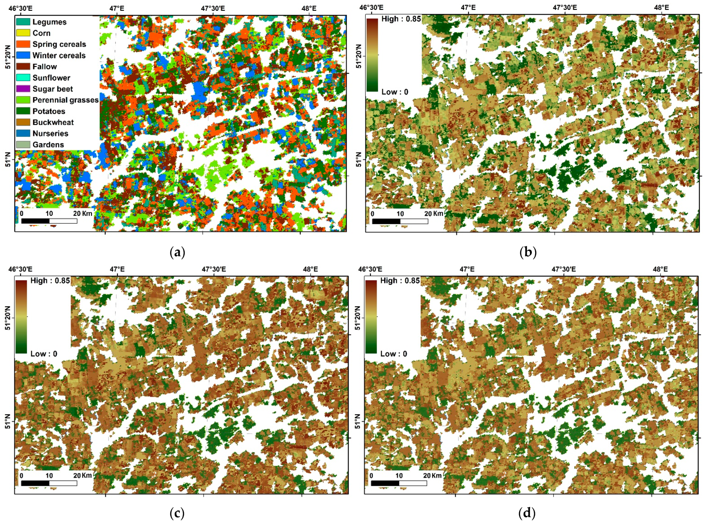
2.3.1. C-Factor Assessment on Arable Land
2.3.2. C-Factor Assessment on Non-Arable Land
3. Results and Discussion
4. Conclusions
Author Contributions
Funding
Institutional Review Board Statement
Informed Consent Statement
Data Availability Statement
Conflicts of Interest
References
- Golosov, V.; Yermolaev, O.; Rysin, I.; Vanmaercke, M.; Medvedeva, R.; Zaytseva, M. Mapping and spatial-temporal assessment of gully density in the Middle Volga region, Russia. Earth Surf. Process. Landforms 2018, 43, 2818–2834. [Google Scholar] [CrossRef]
- Larionov, G.A. Soil Erosion and Deflation; Moscow State University Publishing House: Moscow, Russia, 1993; p. 200. (In Russian) [Google Scholar]
- Litvin, L.F. Geography of Soil Erosion of Agricultural Lands in Russia; Akademkniga: Moscow, Russia, 2002; p. 256. (In Russian) [Google Scholar]
- Lisetskiy, F.N.; Svetlichnyi, A.A.; Chornyy, S.G. Recent Developments in Erosion Science; Konstanta: Belgorod, Russia, 2012; p. 456. (In Russian) [Google Scholar]
- Catchment Erosion-Fluvial Systems: Monograph; Chalov, R.S.; Sidorchuk, A.Y.; Golosov, V.N. (Eds.) INFRA-M: Moscow, Russia, 2017; p. 702. (In Russian) [Google Scholar]
- Feng, Q.; Zhao, W.; Ding, J.; Fang, X.; Zhang, X. Estimation of the cover and management factor based on stratified coverage and remote sensing indices: A case study in the Loess Plateau of China. J. Soils Sediments 2017, 18, 775–790. [Google Scholar] [CrossRef]
- Wischmeier, W.H.; Smith, D.D. Predicting rainfall erosion losses: A guide to conservation planning with Universal Soil Loss Equation (USLE). In Agriculture Handbook; Department of Agriculture: Washington, DC, USA, 1978. [Google Scholar]
- Renard, K.G.; Foster, G.R.; Weesies, G.A.; McCool, D.K.; Yoder, D.C. Predicting Soil Erosion by Water: A Guide to Conservation Planning with the Revised Universal Soil Loss Equation (RUSLE). In Agriculture Handbook; USDA-ARS: Washington, DC, USA, 1997. [Google Scholar]
- Beasley, D.B.; Huggins, L.F.; Monke, E.J. ANSWERS: A Model for Watershed Planning. Trans. ASAE 1980, 23, 0938–0944. [Google Scholar] [CrossRef]
- Palazón, L.; Navas, A. Sediment production of an alpine catchment with SWAT. Z. Für Geomorphol. Suppl. Issues 2013, 57, 69–85. [Google Scholar] [CrossRef] [Green Version]
- De Jong, S.; Paracchini, M.; Bertolo, F.; Folving, S.; Megier, J.; de Roo, A. Regional assessment of soil erosion using the distributed model SEMMED and remotely sensed data. Catena 1999, 37, 291–308. [Google Scholar] [CrossRef]
- Fernández, C.; Vega, J.A.; Vieira, D. Assessing soil erosion after fire and rehabilitation treatments in NW Spain: Performance of rusle and revised Morgan-Morgan-Finney models. Land Degrad. Dev. 2010, 21, 58–67. [Google Scholar] [CrossRef] [Green Version]
- Cohen, M.J.; Shepherd, K.; Walsh, M.G. Empirical reformulation of the universal soil loss equation for erosion risk assessment in a tropical watershed. Geoderma 2005, 124, 235–252. [Google Scholar] [CrossRef]
- Fu, B.J.; Zhao, W.; Chen, L.D.; Zhang, Q.J.; Lü, Y.H.; Gulinck, H.; Poesen, J. Assessment of soil erosion at large watershed scale using RUSLE and GIS: A case study in the Loess Plateau of China. Land Degrad. Dev. 2005, 16, 73–85. [Google Scholar] [CrossRef]
- Lu, D.; Li, G.; Valladares, G.S.; Batistella, M. Mapping soil erosion risk in Rondônia, Brazilian Amazonia: Using RUSLE, remote sensing and GIS. Land Degrad. Dev. 2004, 15, 499–512. [Google Scholar] [CrossRef]
- Panagos, P.; Borrelli, P.; Meusburger, K.; Alewell, C.; Lugato, E.; Montanarella, L. Estimating the soil erosion cover-management factor at the European scale. Land Use Policy 2015, 48, 38–50. [Google Scholar] [CrossRef]
- Panagos, P.; Borrelli, P.; Poesen, J.; Meusburger, K.; Ballabio, C.; Lugato, E.; Montanarella, L.; Alewell, C. Reply to the comment on “The new assessment of soil loss by water erosion in Europe” by Fiener & Auerswald. Environ. Sci. Policy 2016, 57, 143–150. [Google Scholar] [CrossRef]
- Zharkova, Y.G. Soil-Protective Properties of Agrocenoses. In Proceedings of the Conference “Working of Water Streams”; MSU Publishing House: Moscow, Russia, 1987; pp. 39–51. (In Russian) [Google Scholar]
- Zaslavsky, M.N. Erosion Study; Vysshaya shkola: Moscow, Russia, 1983; p. 320. (In Russian) [Google Scholar]
- Morgun, F.T.; Shikula, N.K.; Tararico, A.G. Conservation Agriculture; Urozhay: Kiev, Ukraine, 1988; p. 256. (In Russian) [Google Scholar]
- Maltsev, K.; Yermolaev, O. Assessment of soil loss by water erosion in small river basins in Russia. Catena 2020, 195, 104726. [Google Scholar] [CrossRef]
- Bartsch, K.; Miegroet, H.; Boettinger, J.; Dobrowolski, J. Using Empirical Erosion Models and GIS to Determine Erosion Risk at Camp Williams, Utah. J. Soil Water Conserv. 2002, 57, 29–37. [Google Scholar]
- Bhuyan, S.J.; Kalita, P.K.; A. Janssen, K.; Barnes, P.L. Soil loss predictions with three erosion simulation models. Environ. Model. Softw. 2002, 17, 135–144. [Google Scholar] [CrossRef]
- Fu, G.; Chen, S.; McCool, D.K. Modeling the impacts of no-till practice on soil erosion and sediment yield with RUSLE, SEDD, and ArcView GIS. Soil Tillage Res. 2006, 85, 38–49. [Google Scholar] [CrossRef]
- Beskow, S.; de Mello, C.; Norton, L.; Curi, N.; Viola, M.R.; Avanzi, J. Soil erosion prediction in the Grande River Basin, Brazil using distributed modeling. Catena 2009, 79, 49–59. [Google Scholar] [CrossRef]
- Terranova, O.; Antronico, L.; Coscarelli, R.; Iaquinta, P. Soil erosion risk scenarios in the Mediterranean environment using RUSLE and GIS: An application model for Calabria (southern Italy). Geomorphology 2009, 112, 228–245. [Google Scholar] [CrossRef]
- Park, S.; Oh, C.; Jeon, S.; Jung, H.; Choi, C. Soil erosion risk in Korean watersheds, assessed using the revised universal soil loss equation. J. Hydrol. 2011, 399, 263–273. [Google Scholar] [CrossRef]
- Ranzi, R.; Le, T.H.; Rulli, M.C. A RUSLE approach to model suspended sediment load in the Lo river (Vietnam): Effects of reservoirs and land use changes. J. Hydrol. 2012, 422–423, 17–29. [Google Scholar] [CrossRef]
- Zhao, W.; Fu, B.; Qiu, Y. An Upscaling Method for Cover-Management Factor and Its Application in the Loess Plateau of China. Int. J. Environ. Res. Public Health 2013, 10, 4752–4766. [Google Scholar] [CrossRef] [Green Version]
- Fiener, P.; Auerswald, K. Comment on The new assessment of soil loss by water erosion in Europe. Panagos P. et al., 2015 Environmental Science & Policy 54, 438–447—A response. Environ. Sci. Policy 2016, 57, 140–142. [Google Scholar] [CrossRef]
- De Jong, S.M. Derivation of vegetative variables from a landsat tm image for modelling soil erosion. Earth Surf. Process. Landforms 1994, 19, 165–178. [Google Scholar] [CrossRef]
- Knijff, J.; Jones, R.; Montanarella, L. Soil Erosion Risk Assessment in Europe; JRC, European Soil Bureau. 2000, p. 36. Available online: https://esdac.jrc.ec.europa.eu/content/soil-erosion-risk-assessment-europe (accessed on 15 September 2021).
- Wang, G.; Wente, S.; Gertner, G.Z.; Anderson, A. Improvement in mapping vegetation cover factor for the universal soil loss equation by geostatistical methods with Landsat Thematic Mapper images. Int. J. Remote Sens. 2002, 23, 3649–3667. [Google Scholar] [CrossRef]
- Warren, S.D.; Mitasova, H.; Hohmann, M.G.; Landsberger, S.; Iskander, F.Y.; Ruzycki, T.S.; Senseman, G.M. Validation of a 3-D enhancement of the Universal Soil Loss Equation for prediction of soil erosion and sediment deposition. Catena 2005, 64, 281–296. [Google Scholar] [CrossRef]
- De Asis, A.M.; Omasa, K. Estimation of vegetation parameter for modeling soil erosion using linear Spectral Mixture Analysis of Landsat ETM data. ISPRS J. Photogramm. Remote Sens. 2007, 62, 309–324. [Google Scholar] [CrossRef]
- Suriyaprasita, M.; Shrestha, D.P. Deriving Land Use and Canopy Cover Factor from Remote Sensing and Field Data in Inaccessible Mountainous Terrain for Use in Soil Erosion Modeling. Int. Arch. Photogramm. Remote Sens. Spat. Inf. Sci. 2008, 37, 1747–1750. [Google Scholar]
- Baret, F.; Guyot, G. Potentials and limits of vegetation indices for LAI and APAR assessment. Remote Sens. Environ. 1991, 35, 161–173. [Google Scholar] [CrossRef]
- Richardsons, A.J.; Wiegand, A. Distinguishing Vegetation from Soil Background Information. Photogramm. Eng. Remote Sens. 1977, 43, 1541–1552. [Google Scholar]
- Cyr, L.; Bonn, F.; Pesant, A. Vegetation indices derived from remote sensing for an estimation of soil protection against water erosion. Ecol. Model. 1995, 79, 277–285. [Google Scholar] [CrossRef]
- Cartagena, D.F. Remotely Sensed Land Cover Parameter Extraction for Watershed Erosion Modeling; International Institute for Geo-Information and Earth Observation: Enschede, The Netherlands, 2004; p. 104. [Google Scholar]
- Kefi, M.; Yoshino, K.; Setiawan, Y. Assessment and mapping of soil erosion risk by water in Tunisia using time series MODIS data. Paddy Water Environ. 2012, 10, 59–73. [Google Scholar] [CrossRef]
- Alexandridis, T.; Sotiropoulou, A.M.; Bilas, G.; Karapetsas, N.; Silleos, N.G. The Effects of Seasonality in Estimating the C-Factor of Soil Erosion Studies. Land Degrad. Dev. 2013, 26, 596–603. [Google Scholar] [CrossRef]
- Bartalev, S.A.; Egorov, V.A.; Zharko, V.O.; Loupian, E.A.; Plotnikov, D.E.; Khvostikov, S.A. State and Per-Spectives of the Development of Methods for Satellite Mapping of Vegetation Cover in Russia. Sovremennye Problemy Distantsionnogo Zondirovaniya Zemli Kosmosa 2015, 12, 203–221. (In Russian) [Google Scholar]
- Yermolaev, O.; Mukharamova, S.; Vedeneeva, E. River runoff modeling in the European territory of Russia. Catena 2021, 203, 105327. [Google Scholar] [CrossRef]
- Bartalev, S.; Egorov, V.; Zharko, V.; Loupian, E.; Plotnikov, D.; Khvostikov, S.; Shabanov, N. Land Cover Mapping over Russia Using Earth Observation Data; Russian Academy of Sciences’ Space Research Institute: Moscow, Russia, 2016. [Google Scholar]
- Saveliev, A.; Romanov, A.V.; Mukharamova, S.S. Automated Mapping using Multilevel B-Splines. Appl. GIS 2005, 1. [Google Scholar] [CrossRef]
- Fisette, T.; Rollin, P.; Aly, Z.; Campbell, L.; Daneshfar, B.; Filyer, P.; Smith, A.; Davidson, A.; Shang, J.; Jarvis, I. AAFC annual crop inventory. In Proceedings of the 2013 Second International Conference on Agro-Geoinformatics (Agro-Geoinformatics); Institute of Electrical and Electronics Engineers (IEEE), Fairfax, VA, USA, 12–16 August 2013; pp. 270–274. [Google Scholar]
- Schmidhuber, J. Deep learning in neural networks: An overview. Neural Netw. 2015, 61, 85–117. [Google Scholar] [CrossRef] [Green Version]
- Breiman, L. Random Forests. Mach. Learn. 2001, 45, 5–32. [Google Scholar] [CrossRef] [Green Version]
- Hochreiter, S.; Schmidhuber, J. Long short-term memory. Neural Comput. 1997, 9, 1735–1780. [Google Scholar] [CrossRef] [PubMed]
- Litvin, L.F.; Kiryukhina, Z.P.; Krasnov, S.F.; Dobrovol’Skaya, N.G. Dynamics of agricultural soil erosion in European Russia. Eurasian Soil Sci. 2017, 50, 1344–1353. [Google Scholar] [CrossRef]
- De Jong, S.M.; Brouwer, L.C.; Riezebos, H.T. Erosion Hazard Assessment in the La Peyne Catchment, France; Department of Physical Geography, University of Utrecht: Utrecht, The Netherlands, 1998. [Google Scholar]
- Schmidt, S.; Alewell, C.; Meusburger, K. Mapping spatio-temporal dynamics of the cover and management factor (C-factor) for grasslands in Switzerland. Remote Sens. Environ. 2018, 211, 89–104. [Google Scholar] [CrossRef]
- Grauso, S.; Verrubbi, V.; Peloso, A.; Sciortino, M.; Zini, A. Estimating the C-Factor of USLE/RUSLE by Means of NDVI Time-Series in Southern Latium. An Improved Correlation Model; Italian National Agency For New Technologies, Energy and Sustainable Economic Development: Roma, Italy, 2018; p. 32. [Google Scholar]


| Methods | MLP | RF | LSTM | |
|---|---|---|---|---|
| Crops | Correct Recognition Percentage | |||
| Legumes | 49.8 | 23.1 | 79.5 | |
| Corn | 77.8 | 0.0 | 94.5 | |
| Spring cereals | 37.1 | 97.9 | 96.4 | |
| Winter wheat | 94.5 | 4.6 | 93.1 | |
| Fallow | 42.4 | 40.4 | 87.0 | |
| Sunflower | 18.0 | 0.0 | 95.4 | |
| Sugar beet | 90.0 | 0.0 | 100.0 | |
| Perennial grasses | 14.6 | 94.6 | 95.1 | |
| Potatoes | 59.8 | 0.0 | 98.7 | |
| Buckwheat | 34.8 | 0.0 | 100.0 | |
| Average percentage of correct recognition (taking into account the representativeness of crop classes) | 40 | 90 | 94 | |
| Crops | Pearson Correlation Coefficient | Statistics of Area Differences, (ha) | Frequency Histograms of the Area Differences, (ha) | Agreement of Areas, (ha) (Vertical Axis-Results of Recognition; Horizontal Axis–Rosstat Data) | |
|---|---|---|---|---|---|
| Entire sown area | 0.96 | Median | 98 | 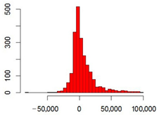 |  |
| Mean | 4800 | ||||
| 1st quartile | −5300 | ||||
| 3rd quartile | 10,000 | ||||
| Cereal and Legumes | 0.90 | Median | −6900 | 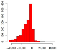 | 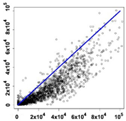 |
| Mean | −9500 | ||||
| 1st quartile | −15,160 | ||||
| 3rd quartile | −1600 | ||||
| Winter cereal | 0.91 | Median | −160 |  |  |
| Mean | −230 | ||||
| 1st quartile | −2700 | ||||
| 3rd quartile | −1030 | ||||
| Legumes | 0.50 | Median | 230 |  |  |
| Mean | 900 | ||||
| 1st quartile | −17 | ||||
| 3rd quartile | 1460 | ||||
| Crops, Groups of Crops | Periods | Sigmoid Parameters | ||||||||
|---|---|---|---|---|---|---|---|---|---|---|
| ID | C1 | C2 | C3 | C4 | C5 | C6 | a | b | c | |
| Legumes | 1 | 0.55 | 0.74 | 0.64 | 0.35 | 0.08 | 0.20 | 0.74 | 0.62 | −0.15 |
| Corn | 2 | 0.77 | 0.83 | 0.71 | 0.50 | 0.27 | 0.45 | 0.89 | 0.70 | −0.26 |
| Spring cereals and annual grasses | 3 | 0.55 | 0.74 | 0.64 | 0.35 | 0.08 | 0.20 | 0.74 | 0.62 | −0.15 |
| Winter cereals | 4 | 0.64 | 0.64 | 0.64 | 0.35 | 0.08 | 0.20 | 0.74 | 0.62 | −0.15 |
| Fallow | 6 | 0.62 | 0.60 | 0.57 | 0.54 | 0.50 | 0.50 | 0.69 | 1.84 | −0.94 |
| Sunflower | 7 | 0.77 | 0.83 | 0.71 | 0.50 | 0.27 | 0.45 | 0.89 | 0.70 | −0.26 |
| Sugar beet | 8 | 0.77 | 0.83 | 0.76 | 0.63 | 0.40 | 0.60 | 0.84 | 0.88 | −0.22 |
| Potatoes | 10 | 0.77 | 0.83 | 0.66 | 0.46 | 0.26 | 0.60 | 1.04 | 0.53 | −0.36 |
| Buckwheat | 11 | 0.55 | 0.74 | 0.64 | 0.35 | 0.08 | 0.20 | 0.74 | 0.62 | −0.15 |
| Crops | Model Plot | Prameters Values | Approximation Quality |
|---|---|---|---|
| Legumes | 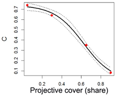 | a = 0.74 b = 0.62 c = −0.15 | Adjusted R-squared: 0.99 |
| Corn, Sunflower | 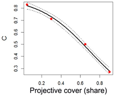 | a = 0.89 b = 0.70 c = −0.26 | Adjusted R-squared: 0.99 |
| Sugar beet | 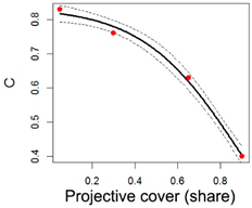 | a = 0.84 b = 0.88 c = −0.22 | Adjusted R-squared: 0.99 |
| Potatoes |  | a = 1.04 b = 0.53 c = −0.36 | Adjusted R-squared: 0.99 |
| Fallow | 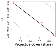 | a = 0.68 b = 1.83 c = −0.94 | Adjusted R-squared: 0.98 |
| Code | Land Cover Type TerraNorte RLC | Description | C-Factor Minimum | C-Factor Maximum |
|---|---|---|---|---|
| 1 | Dark coniferous evergreen forests | Forests, in the canopy of which at least 80% of the crown area is shade-tolerant species of coniferous trees, including spruce, fir, and Siberian pine (cedar). | 0.0001 | 0.003 |
| 2 | Light coniferous evergreen forests | Forests, in the canopy of which at least 80% of the crown area is Scots pine. | 0.0001 | 0.003 |
| 3 | Deciduous forests | In the canopy, at least 80% of the area is occupied by crowns of birch and aspen, as well as broad-leaved species, including oak, linden, ash, maple, elm, and some other species. | 0.0001 | 0.003 |
| 10 | Mixed forests with a predominance of conifers | Crowns of coniferous trees occupy from 60 to 80%, deciduous trees from 20% to 40% of the canopy area. | 0.0001 | 0.003 |
| 11 | Mixed forests | Crown areas of coniferous and deciduous trees are presented in approximately equal proportions (40–60%) in the canopy. | 0.0001 | 0.003 |
| 12 | Mixed forests with a predominance of deciduous | Crowns of deciduous trees occupy from 60–80%, conifers from 20% to 40% of the canopy area. | 0.0001 | 0.003 |
| 4 | Coniferous deciduous (larch) forests | In the canopy of forests, the crowns of larch trees occupy more than 80% of the area. | 0.0001 | 0.003 |
| 23 | Sparse coniferous deciduous (larch) | Areas occupied by detached trees or sparse plantations of larch with a projective crown cover of less than 20%. | 0.003 | 0.05 |
| 8 | Natural grasslands | Grass vegetation with a growing season of more than 5 months. The species composition is characterized by the predominance of perennial grasses, mainly grasses, and sedges, in conditions of sufficient moisture. The area of the projection of crowns of trees and shrubs is less than 20%. | 0.01 | 0.15 |
| 14 | Steppe | The grass cover is formed mainly by drought-resistant perennial sod grasses (feather grass, fescue, wormwood, wheatgrass, etc.). There is a wide variety of species of steppe shrubs and semi-shrubs, as well as short-flowering ephemeroids and ephemerals. | 0.01 | 0.45 |
| 5 | Coniferous evergreen shrubs | Shrubs or low-stemmed dwarf cedar forests. | 0.003 | 0.1 |
| 9 | Deciduous shrubs | A community of low-growing or creeping shrubs (shrub or dwarf birches, polar willows, etc.). | 0.003 | 0.1 |
| 16 | Subshrub tundra | Dry tundra with rare fragmented vegetation, dominated by species of Alp-Arctic shrub communities less than 15 cm in height. Moss-lichen cover and forbs are also widespread. | 0.1 | 0.45 |
| 17 | Grassy tundra | The tundra is represented mainly by various species of grasses and mosses growing on moist soils and forming a continuous vegetation cover. Shrubs up to 40 cm in height are often found. | 0.1 | 0.45 |
| 18 | Subshrub tundra 2 | Shrubs (dwarf birch and various species of willow) dominate with a height of more than 40 cm, sometimes with an admixture of juniper, alder, or dwarf pine. | 0.1 | 0.45 |
| 24 | Recent burnt area | Forests and tundra vegetation destroyed or damaged by fire. | 0.1 | 0.55 |
| C-Factor, 2010 | C-Factor, 2012–2014 | C-Factor According to the Research Results | % Change from 2010 | % Change from 2012–2014 | |
|---|---|---|---|---|---|
| European part of Russia | 0.4 | - | 0.401 | 0 | - |
| Landscape zones: | |||||
| Northern and middle taiga | 0.19 | 0.18 | 0.171 | −10 | −5 |
| South taiga | 0.22 | 0.23 | 0.265 | 20 | 15 |
| Forest area | 0.22 | 0.23 | 0.262 | 19 | 14 |
| Forest-steppe | 0.40 | 0.38 | 0.362 | −10 | −5 |
| Steppe | 0.45 | 0.43 | 0.454 | 1 | 5 |
Publisher’s Note: MDPI stays neutral with regard to jurisdictional claims in published maps and institutional affiliations. |
© 2021 by the authors. Licensee MDPI, Basel, Switzerland. This article is an open access article distributed under the terms and conditions of the Creative Commons Attribution (CC BY) license (https://creativecommons.org/licenses/by/4.0/).
Share and Cite
Mukharamova, S.; Saveliev, A.; Ivanov, M.; Gafurov, A.; Yermolaev, O. Estimating the Soil Erosion Cover-Management Factor at the European Part of Russia. ISPRS Int. J. Geo-Inf. 2021, 10, 645. https://doi.org/10.3390/ijgi10100645
Mukharamova S, Saveliev A, Ivanov M, Gafurov A, Yermolaev O. Estimating the Soil Erosion Cover-Management Factor at the European Part of Russia. ISPRS International Journal of Geo-Information. 2021; 10(10):645. https://doi.org/10.3390/ijgi10100645
Chicago/Turabian StyleMukharamova, Svetlana, Anatoly Saveliev, Maxim Ivanov, Artur Gafurov, and Oleg Yermolaev. 2021. "Estimating the Soil Erosion Cover-Management Factor at the European Part of Russia" ISPRS International Journal of Geo-Information 10, no. 10: 645. https://doi.org/10.3390/ijgi10100645