Development of a New Phenology Algorithm for Fine Mapping of Cropping Intensity in Complex Planting Areas Using Sentinel-2 and Google Earth Engine

Abstract

Cropping intensity is a key indicator for evaluating grain production and intensive use of cropland. Timely and accurately monitoring of cropping intensity is of great significance for ensuring national food security and improving the level of national land management. In this study, we used all Sentinel-2 images on the Google Earth Engine cloud platform, and constructed an improved peak point detection method to extract the cropping intensity of a heterogeneous planting area combined with crop phenology. The crop growth cycle profiles were extracted from the multi-temporal normalized difference vegetation index (NDVI) and land surface water index (LSWI) datasets. Results show that by 2020, the area of single cropping, double cropping, and triple cropping in the Henan Province are 52,236.9 km², 74,334.1 km², and 1927.1 km², respectively; the corresponding producer accuracies are 86.12%, 93.72%, and 91.41%, respectively; the corresponding user accuracies are 88.99%, 92.29%, and 71.26%, respectively. The overall accuracy is 90.95%, and the Kappa coefficient is 0.81. Using the sown area in the statistical yearbook data of cities in the Henan Province to verify the extraction results of this paper, the R² is 0.9717, and the root mean square error is 1715.9 km². This study shows that using all the Sentinel-2 data, the phenology algorithm, and cloud computing technology has great potential in producing a high spatio-temporal resolution dataset for crop remote sensing monitoring and agricultural policymaking in complex planting areas.

1. Introduction

The “17 Sustainable Development Goals” (SDGs) issued by the United Nations in 2015 clearly took eliminating hunger and achieving food security as one of its goals and tasks. Therefore, with the rapid growth of the population and economy, how to ensure food security remains the focus of attention of governments and the international community [1,2,3]. The main ways to ensure food security include expanding the area of cropland, increasing the yield per unit area, and increasing the degree of intensification of cropland [4]. Under the background of the decline of cropland area in the Peoples’ Republic of China (PRC) [5,6] and the “ceiling effect” of grain yields [7], increasing the degree of cropland intensification has become a key way to increase food production and ensure food security [8]. Cropping intensity is a key indicator to measure the degree of cropland intensification, timely and accurately monitor regional food production, and help achieve SDGs [1,2,9,10].

Remote sensing can fully reflect the spectral differences and phenological characteristics of different crops. At the same time, with the availability of satellite images with different resolutions greatly improved, considerable progress has been made in the production of cropping intensity distribution maps based on remote sensing [11,12]. Over the past few decades, cropping intensity maps have been drawn in different regions using satellite data, such as Brazil [13,14], China [5,15], India [16,17], Arizona [18]. From the selected data sources, the most commonly used satellite data for monitoring cropping intensity are MODIS data and Landsat data. MODIS data have high temporal resolution (1-d), but the spatial resolution is low (250 m to 1000 m). A large number of mixed pixels are difficult to describe the changes in ground crops’ details accurately [19,20,21], so it is more suitable for long-term large-scale regional monitoring. Landsat data have high spatial resolution (30-m) and low temporal resolution (8-d to 16-d). Therefore, it is difficult to obtain high-temporal-resolution data of continuous time series [22,23,24,25]. Sentinel-2A/B data not only have high temporal resolution (5-d to 10-d), but also high spatial resolution (10-m to 60-m), which provides more detailed phenological information for monitoring cropping intensity [26]. This provides the possibility to describe many small-scale farmland areas accurately [27]. Thus, it is necessary to evaluate the potential of Sentinel-2A/B data in cropping intensity monitoring and provide new ideas for the fine mapping of cropping intensity in complex planting areas.

From the selected classification approaches, it can be roughly divided into: (1) image-based spatial statistics and (2) pixel-based temporal statistics. Regarding (1), previous studies extracted cropping intensity based on the differences in the spectrum [28] or vegetation index (VIs) [29,30] in a specific time window, which can best reflect the growth characteristics of the crops. This classification approach needs to collect a wide range of training samples, which not only consumes a lot of time and manpower, but also the quantity and quality of sample points have a great impact on the classification accuracy. Furthermore, due to the influence of atmosphere, clouds, cloud shadow, etc., it is difficult to obtain crop growth characteristics accurately. Regarding (2), this approach generates a cropping intensity map using rule-based algorithms based on constructed time series datasets of VIs [31,32,33,34]. These VIs include the normalized difference vegetation index (NDVI) [14,35], enhanced vegetation index (EVI) [36,37], land surface water index (LSWI) [16], and modified normalized difference water index (mNDWI) [38,39]. This approach is based on the crop phenological characteristics recorded in the VIs’ time series. By analyzing the life cycle of the crop, the temporal metrics of crops are obtained, and the classification rules are generated [39,40,41].

Vegetation phenology is a natural phenomenon that reflects the annual cycle of plants under the influence of biological and non-biological factors [25]. Previous studies have proved that crop phenology algorithms have great potential in agricultural remote sensing mapping, such as identifying the start of season (SOS) and the end of season (EOS) [15], identifying the peak growth (PG) and peak drought (PD) periods [42], calculating the length of the growth cycle [43], calculating the growth rate and decline rate of VIs’ values [44], and assessing cropping intensity by identifying the number of peaks and troughs in the VIs’ time series within a year [5,16,31,45]. A recent study used the NDVI threshold to distinguish between crops and natural vegetation, and used the LSWI threshold to identify bare soil to map the cropping intensity of seven representative grain producing areas in China successfully [46]. In intercropping areas, the next crop is usually sown when the previous crop is not harvested, which results in the bare soil being not being recognized between the harvest and sowing of the two crops. Another study only used the NDVI time series dataset to construct a binary crop phenology profile indicating the growth and non-growth periods, and mapped global cropping intensity at 30 m resolution [47]. The 50% NDVI amplitude threshold was used as a key node in identifying crop growth cycles in this algorithm. However, multiple crop rotations and intercropping systems in various regions will affect the accuracy and reliability of the results. Thus, there is a need to develop a new phenology-based algorithm to identify cropping intensity in complex planting areas.

At present, mapping the cropping intensity over any sizeable region is still a challenge, especially for complex planting areas (e.g., the Henan Province in PRC (details on this region are given in the methods section below)). Firstly, the frequency and dates of high-quality images vary greatly in time and space due to the influence of the atmosphere, clouds, cloud shadows, etc. Under normal circumstances, irregular image time series are usually difficult to support the development of classification models [48,49]. Secondly, crop management measures in different regions lead to high intra-class variabilities of crop spectrum and phenology in the Henan Province. For example, in Qixian and Tongxu, Henan Province, corn is sown in some areas in mid-April, and a considerable part of corn is sown in early June. In many of these areas, crop rotation management is implemented, and the dates of crop planting and harvesting vary greatly in the same year and in different years. Therefore, only using a specific time window as the study interval cannot accurately capture the complete dynamic changes of crop growth [30]. Thirdly, winter crops usually have two peaks in one growing season. Therefore, only extracting the peak numbers of VIs’ time series to quantify cropping intensity can easily lead to overestimation of the results.

Considering the limitations of using remote sensing to identify cropping intensity in complex planting areas, we developed a phenological-based algorithm on the Google Earth Engine (GEE) cloud platform, and applied the algorithm to generate a cropping intensity product with 10 m spatial resolution in the Henan Province in 2020. The algorithm accurately captures the subtle changes of planting systems in cropland, which can be used to produce cropping intensity products with high-resolution, and provides a reference for the monitoring of highly heterogeneous farmland vegetation.

2. Materials and Methods

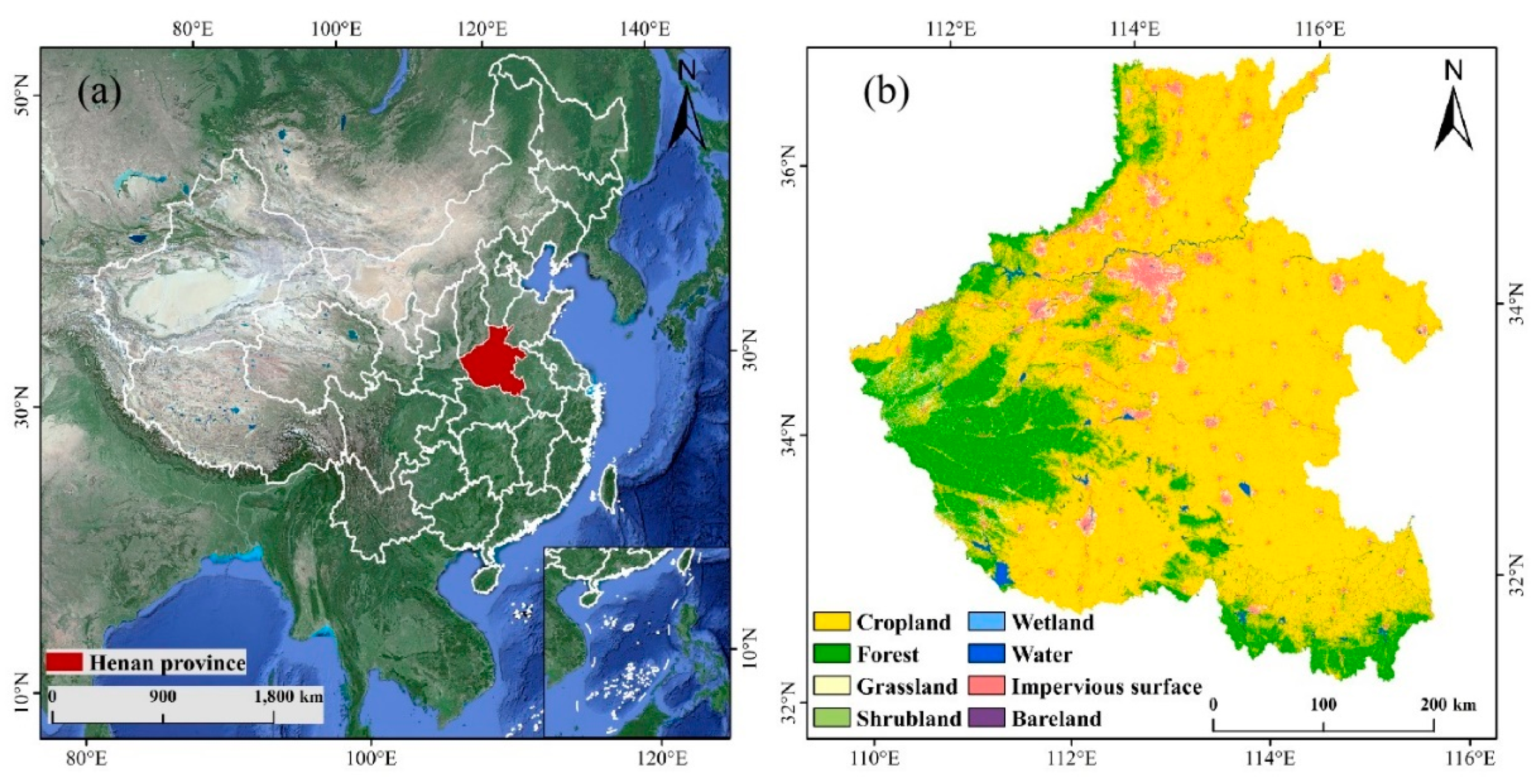
2.1. Study Area

The Henan Province (31°23′~36°22′ N, 110°21′~116°39′ E) is located in the middle-eastern part of PRC, in the middle and lower reaches of the Yellow River, with an area of 6444 km² (Figure 1). The overall terrain is high in the west and low in the east; surrounded by mountains in the south is the North China Plain in the middle east and Nanyang Basin in the southwest. The north of the Henan Province is located in the warm temperate zone, and a small part of the south is located in the subtropical zone, belonging to the continental monsoon climate from the north subtropical to the warm temperate zone. The annual average temperature is 12–16 °C, and the annual average precipitation is 500–900 mm. It crosses the four major water systems of the Haihe River, the Yellow River, the Huaihe River, and the Yangtze River. Abundant light, heat, and water have laid a good foundation for the development of agriculture in the Henan Province. In 2019, the production of grain in the Henan province was 66.953 million tons, accounting for 10.09% of the national grain output (https://data.cnki.net/yearbook/Single/N2021010028 accessed on 1 May 2021). As an important agricultural product production base of PRC, the Henan Province’s main crops are wheat, corn, rice and rape, etc. The cropping system is mainly single cropping and double cropping. Its land use and grain yield are not only related to Henan’s own development, but also of great significance to the national food supply.

2.2. Datasets and Preprocessing

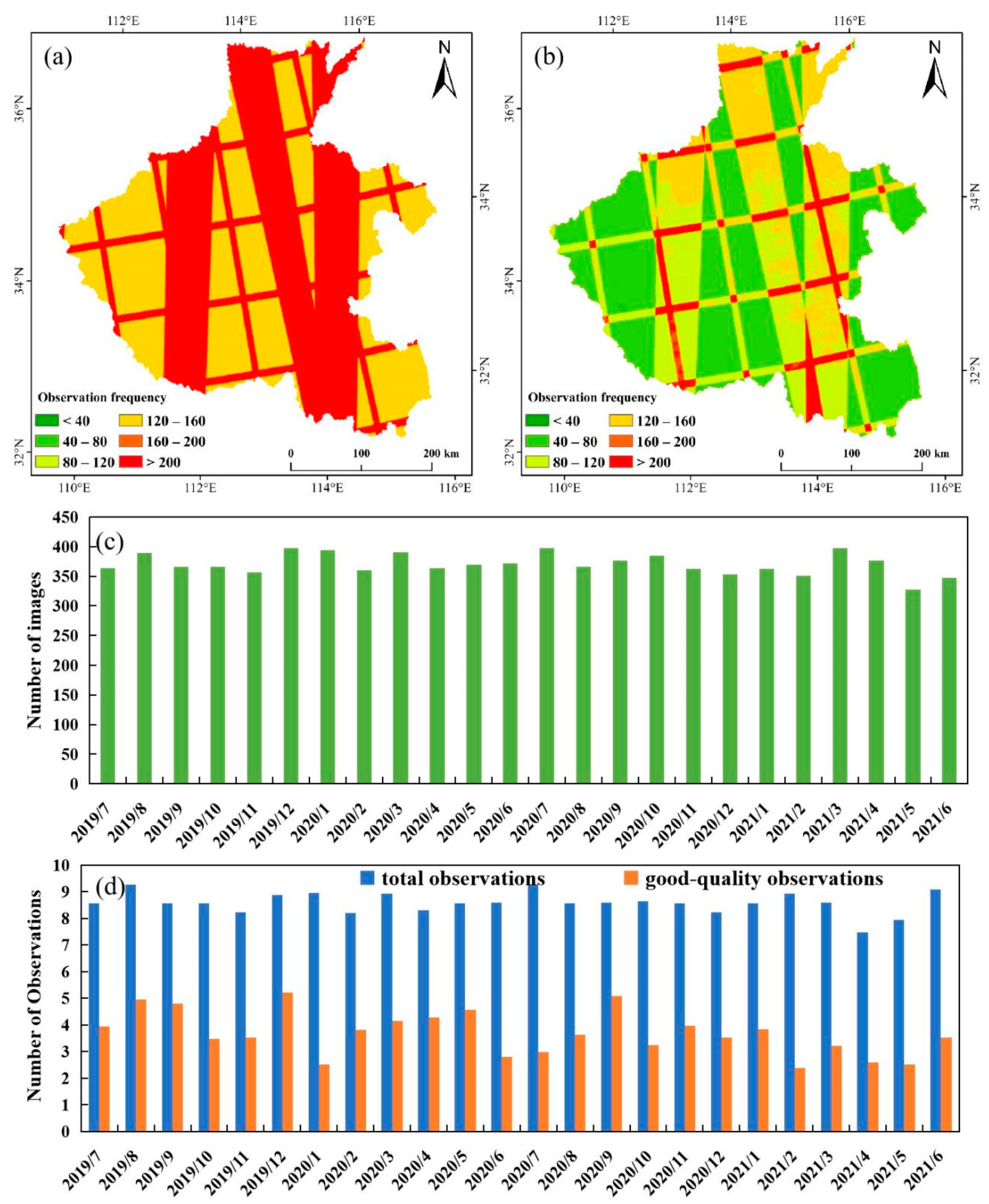
2.2.1. Sentinel-2A/B Imagery

Sentinel-2 is an Earth observation mission of the European Union Copernicus Program. It consists of two satellites, which were launched in June 2015 (Sentinel-2A) and March 2017 (Sentinel-2B). The revisit period of the dual-satellite synchronization is 5 days, and the Multispectral Instrument (MSI) with a spatial resolution of 10 m, 20 m, and 60 m has 13 spectral bands from visible light to short-wave infrared [50]. The GEE cloud platform contains two types of data: Top-of-Atmosphere Reflectance (TOA) and Surface Reflectance (SR). Since TOA data are sensitive to changes in atmospheric composition and have certain limitations, we used all available SR data in the GEE platform from 2019 to 2021, which correspond to “COPERNICUS/S2_SR” in GEE, because the cropping intensity in 2020 included winter crops from 2019 to 2020 and 2020 to 2021.

The presence of clouds, cloud shadows, and snow in the image will affect the spectral bands, and then affect the calculation results of relevant indexes [51,52,53,54]. The quality assessment band (QA60) in the Sentinel-2 metadata was used to mask the image quality and remove clouds and cloud shadows [38].

We collected a total of 8883 images in the Henan Province during the study period (1 July 2019–1 July 2021). After preprocessing the image according to the above steps, we counted the total observations and good-quality observations of each pixel in the Henan Province, respectively (Figure 2a,b). Most pixels had >120 total observations and >40 good-quality observations in the Henan Province. Moreover, we counted available images for the study (Figure 2c) and observations per pixel in the Henan Province every month (Figure 2d). During the study period, there were >300 images per month, and the total observation and good-quality observations of each pixel were more than 7 times and 2 times per month, respectively.

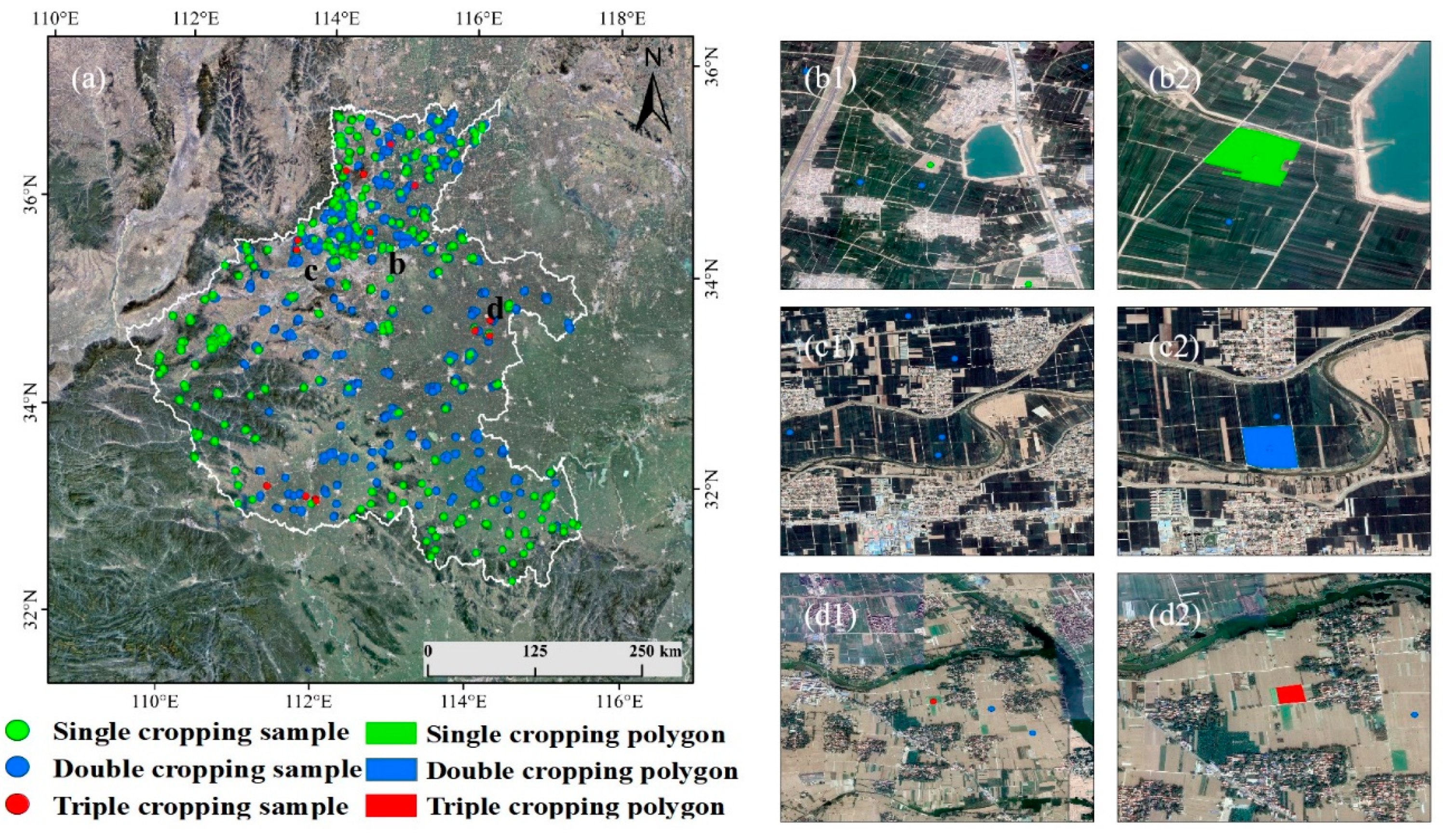
2.2.2. Ground Reference Data

We obtained the reference datasets from three aspects to verify the classification results of this paper. Firstly, based on the Google Earth images with 1 m spatial resolution, the stratified random sampling method was used to obtain single, double, and triple cropping validation samples sets. Secondly, during the period from March to June 2020, we carried out seven field works in Zhengzhou City, Xinxiang City, Kaifeng City, Anyang City, Hebi City, Shangqiu City, Zhoukou City, Xuchang City, Luohe City, and Xinyang City in the Henan Province and collected geo-referenced field photos of different cropping intensities. These field photos include main planting systems such as double cropping of wheat-corn rotation, single cropping of rice, and triple cropping of vegetable. In addition, during field works, we used drones to obtain multispectral images, which were used as auxiliary data in visual interpretation. The spatial resolution of these multi-spectral images can reach 0.1 m, which clearly shows the different planting systems of the land. Finally, we obtained a total of 1219 samples for single cropping, 2131 samples for double cropping, and 22 samples for triple cropping (Figure 3a).

Furthermore, polygonal buffers were generated from the obtained sample points according to the actual shape and size of the farmland (Figure 3b–d). Through random stratified sampling, we collected a total of 1219 polygons (10,971 pixels) for the single cropping system, 2131 polygons (19,179 pixels) for the double cropping system, and 22 polygons (198 pixels) for the triple cropping system. These polygonal buffers were superimposed on Google Earth images, combined with geo-referenced field photos and drone multi-spectral images, and finally obtained single, double, and triple cropping validation grids through visual interpretation.

2.2.3. Other Data

In order to obtain the cropping intensity map accurately, it is necessary to remove the non-cropland pixels in the study area. We used the cropland pixels in the 10 m resolution global land cover product (FROM-GLC10) to mask the constructed good-quality time series datasets, which were published by the Department of Earth System Sciences, Tsinghua University [55]. The map can be freely downloadable from (http://data.ess.tsinghua.edu.cn accessed on 1 May 2021). At the same time, we used statistical data from 17 cities in the Henan Province to compare and analyze the classification results of this paper. The statistical data come from the website of the National Bureau of Statistics (http://www.stats.gov.cn accessed on 1 May 2021).

2.3. Methods

Figure 4 shows the process of extracting cropping intensity in this study. Firstly, we obtained all available Sentinel-2A/B SR data from July 2019 to July 2021 from the GEE platform, and used the quality assessment band (QA60) to remove the bad-quality observations in the Sentinel-2A/B SR data. Secondly, we used a land cover product (FROM-GLC10) with a spatial resolution of 10 m to mask the land in the Henan Province and obtained data on cropland. Thirdly, we calculated the NDVI and LSWI indices of the Henan Province pixel by pixel, and reconstructed the NDVI and LSWI time series, including the 10-day composite, linear interpolation, and Savitzky–Golay filter smoothing (only for NDVI time series). Fourth, combining the LSWI time series and the growth period length (GPL), we eliminated the “false peaks” in the NDVI time series. Finally, according to the number of effective peaks obtained, we determined the cropping intensity of the Henan Province pixel by pixel, and obtained a cropping intensity map of the Henan Province with a spatial resolution of 10 m.

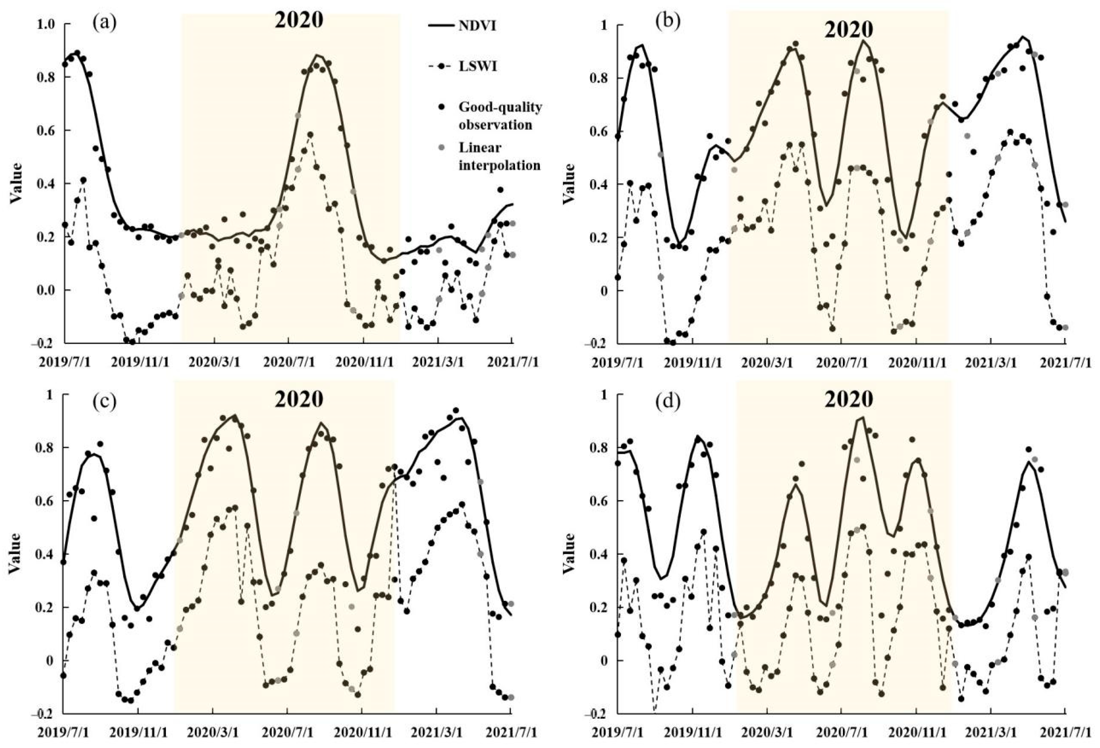
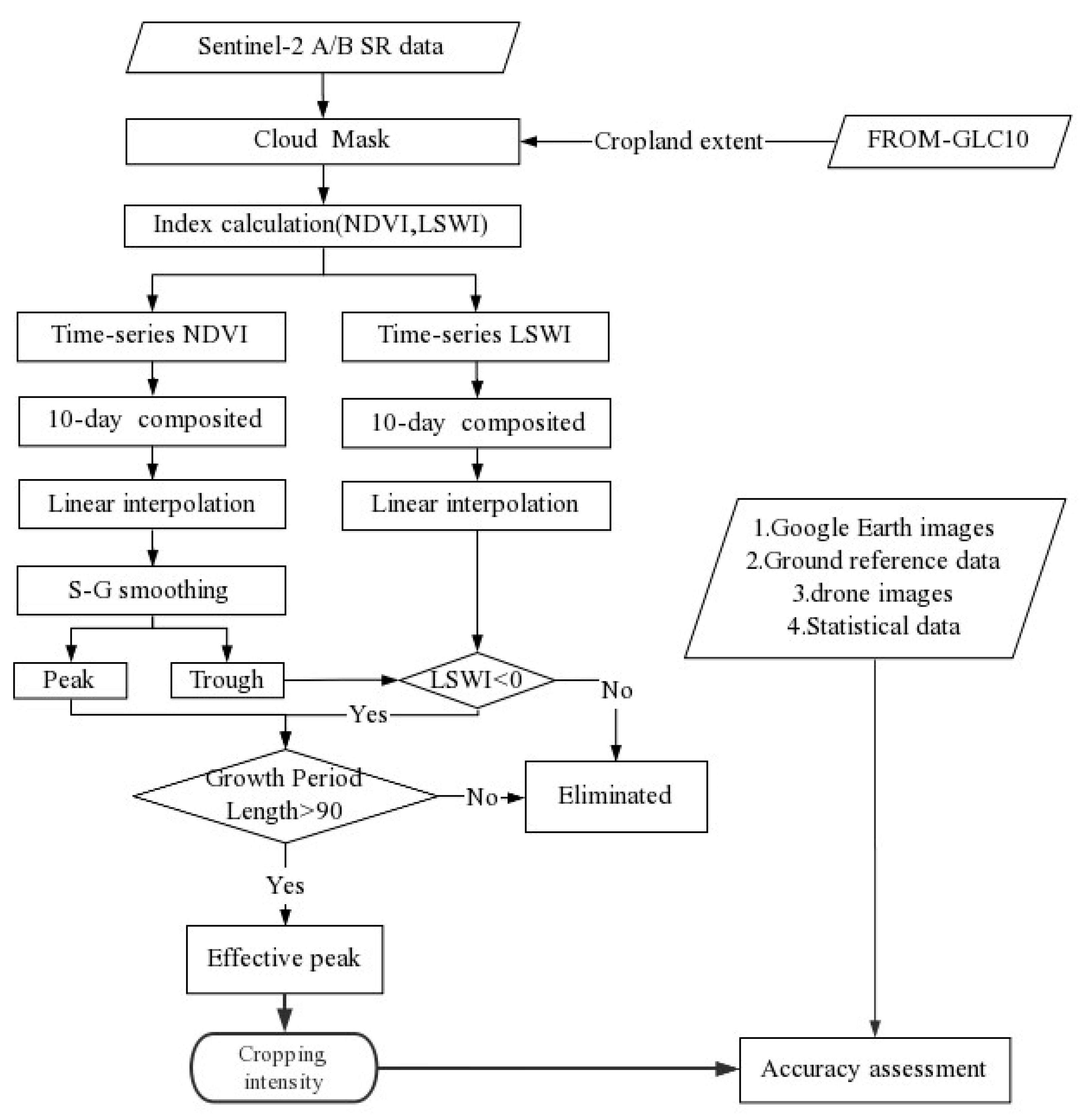
2.3.1. Index Calculation and Time Series Reconstruction

The NDVI value of crops gradually increased from the green-up stage, reaching the maximum value at the peak growth stage, and then decreased from the mature stage to harvest (Figure 5). Therefore, the NDVI index can be used to indicate surface vegetation coverage and growth status. The change trend in the LSWI value during the crop growth period was roughly the same as that of the NDVI value (Figure 5). Soil moisture is much lower than crops, so LSWI values are usually low before crops are planted and after harvest. This can be used to judge the condition of the cropland before sowing and after harvest [56,57]. The calculation formulas of NDVI [58] and LSWI [59] are as follows:

$$\mathrm{NDVI}=\frac{{\mathsf{\rho }}_{\mathrm{NIR}}-{\mathsf{\rho }}_{\mathrm{RED}}}{{\mathsf{\rho }}_{\mathrm{NIR}}+{\mathsf{\rho }}_{\mathrm{RED}}}$$

(1)

$$\mathrm{LSWI}=\frac{{\mathsf{\rho }}_{\mathrm{NIR}}-{\mathsf{\rho }}_{\mathrm{SWIR}}}{{\mathsf{\rho }}_{\mathrm{NIR}}{+\mathsf{\rho }}_{\mathrm{SWIR}}}$$

(2)

where the ${\mathsf{\rho }}_{\mathrm{NIR}}$,${\mathsf{\rho }}_{\mathrm{RED}}$, and ${\mathsf{\rho }}_{\mathrm{SWIR}}$ represent the near infrared band, the red band, and the shortwave infrared band, respectively.

Since the angle of sunlight, the angle of satellite observation, clouds, etc. change greatly over time [60], there is a lot of noise in the original NDVI and LSWI time series data. Thus, the data need to be further processed. We used the following three steps to reconstruct the time series data: (1) Image compositing can reduce the influence of cloud and temporal uneven observation [61,62]. In order to obtain time series of equal lengths and intervals, we calculated the maximum value of the NDVI and the average value of the LSWI every 10 days to generate a composite image for 10 days. The maximum value of the NDVI is selected because the maximum value of the NDVI can reflect the true growth conditions of vegetation during this period, and the average value of the LSWI is selected because the LSWI is very sensitive to changes in soil and vegetation moisture, and the average value of the LSWI is closer to the growth changes in vegetation during that period. After 10 days of compositing processing, we obtained a total of 66 data points (the black dots in Figure 5). (2) Affected by factors such as severe weather, cloud or snow, etc., good-quality observations may not be available in some areas. When there were no good-quality observations in 10 days, based on good-quality observations around 10 days, we used the linear interpolate [63] to fill the gaps in the time series of the NDVI and LSWI. After linear interpolation processing, the available data increased to 77 data points. (3) Even if the NDVI time series data are composited for 10 days, the false high value, the continuous low NDVI value during the synthesis period, and other noise residuals still exist [60], which may cause jagged fluctuations in the NDVI time series. Savitzky–Golay filtering [64] was used to smooth the NDVI dataset (the solid line in Figure 5). Since the growth period of most crops exceeds 90 days, we used a moving window of size 9 and a 2 order of filter [15]. The LSWI is more sensitive to surface moisture, so we did not smooth the LSWI time series.

Based on geo-referenced field photos and Google Earth images, we selected four typical sites representing single, double, and triple cropping intensity. We established time series of NDVI and LSWI values at these sites to obtain phenological indicators of different cropping intensities (Figure 5). Single-cropping crops have a growth cycle within a year, and their NDVI time series usually has only one peak in the year (Figure 5a). Double-cropping crops reach their peak growth stage twice in a year, and their NDVI time series usually has two (Figure 5c) or three peaks (Figure 5b) during the year. For double-cropping rice (Figure 5c) or other non-winter crops double-cropping rotation systems, the NDVI time series usually shows two normal peaks. However, for winter wheat-corn or winter crops and other crops in the double-cropping rotation mode, the NDVI time series has a lower false peak before pre-winter (1 October 2020–1 February 2021) (Figure 5b).

2.3.2. Algorithm for Crop Intensity Mapping

Figure 5 shows that from sowing to harvest, the NDVI curve of the crop first rises to the peak, and then gradually drops to the bottom. This process occurs once in a year for the single cropping area, twice in a year for the double cropping area, and three times in a year for the triple cropping area. Therefore, a growth cycle usually corresponds to a peak (except for winter crops). Then, we use peak detection methods to identify potential peaks (PP) and potential trough (PT) from the crop profile of the NDVI time series in a year. Before and after crops planting, the cropland is bare soil. The LSWI of bare soil is much lower than that of vegetation. Therefore, the LSWI value during the bare soil period can be used to identify the complete growth cycle of the crop [57,65] and eliminate the extra peak value of winter crops.

However, it was obviously unreasonable to determine the cropping intensity of the pixel only based on the number of peaks obtained in the above steps. It is not suitable for the intercropping crop [66]. Crops in intercropping systems usually exhibit two or more crop rotations, and the latter crop is planted when the former crop has not yet been harvested. Therefore, it is impossible to distinguish the two growth cycles of crops using the LSWI to detect bare soil. The double cropping in the intercropping system was incorrectly identified as single cropping. Therefore, we tried to resolve the problem that crops in the intercropping systems are not easy to identify, specifically, the adjacent peaks and the trough between the two peaks in the NDVI time series.

Moreover, the independent growth period of major crops in PRC is more than 90 days [67]. In other words, effective continuous peek recognition must meet 90 days during the crop growth season. The final effective peak (EP) was obtained through the above restriction conditions, and the number of EPs was used to determine the cropping intensity of the pixel. Specific steps are as follows:

• Identified PP and PT through the moving window. In the NDVI time series, when the NDVI value of a certain point was higher (lower) than its two neighboring values, it was judged as the peak (trough) value.
• Marked the PT between two consecutive PPs. In order to avoid identifying the autumn growth of winter wheat and other crops as a separate growth cycle, we used the LSWI value of the crop at PT as one of the limiting conditions for extracting PP. After the crops were harvested, bare soil appeared on the surface pixels, and a growth cycle of the crops ended. Thus, bare soil was an important indicator for judging the complete growth cycle. According to previous studies, due to the low water content of soil in northern PRC, when the LSWI value of a pixel was less than 0 at PTs [16,65], it was recognized as bare soil Equation (3). If the bare soil signal is detected between two consecutive peaks, the two consecutive peaks are identified as two growth cycles.

  $${\mathrm{LSWI}}_{\mathrm{PT}}<0$$

  (3)

  where LSWI_PT is the LSWI value at the potential trough of NDVI.
• Eliminate invalid PPs. Since it is usually difficult to detect LSW in the bare soil period for intercropping crops, we applied a supplementary algorithm to identify its growth cycle. When the NDVI value was between 0.2 and 0.5, the pixels were usually considered to be a mixture of vegetation and bare soil. When the NDVI value was greater than 0.5, the pixels were usually considered as complete vegetation [36,68]. Therefore, for neighboring PPs, if both PPs are greater than 0.5, and the PT between the two PPs is less than 0.5, then both PPs are recorded. Otherwise, only one is recorded; see Equation (4).

  $${\mathrm{NDVI}}_{\mathrm{PPA}}>0.5{\&\mathrm{NDVI}}_{\mathrm{PPB}}>0.5{\&\mathrm{NDVI}}_{\mathrm{PTC}}<0.5$$

  (4)

  where NDVI_PPA and NDVI_PPB are the neighboring potential peak values of the NDVI, and NDVI_PTC is the potential trough value of the NDVI between the NDVI_PPA and NDVI_PPB, respectively.
• Used the growth period length (GPL) to filter the effective PPs further. For crops in intercropping systems, the crop growth cycle should be greater than 90 days. Therefore, when the time span of the wave of the NDVI time series is greater than 90 days, it is recorded as an effective growth cycle, and its peak value is identified by Equation (5).

  GPL > 90

  (5)

  where GPL is the growth period length of crops.
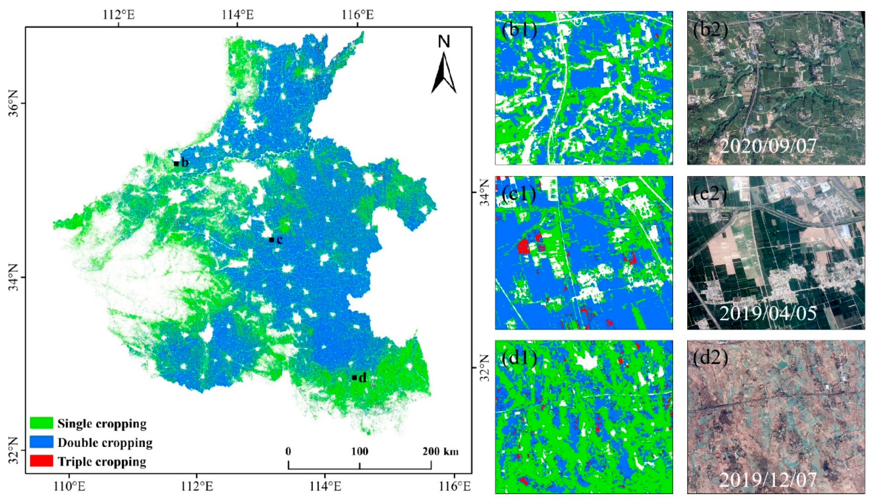
• Based on the number of effective peaks (EP) obtained above, the cropping intensity of each pixel was determined. If there was only 1 EP in a pixel in 2020, it would be marked as a single cropping. If there are 2 or 3 EPs, it would be marked as double cropping or triple cropping. Accordingly, a 10 m spatial resolution cropping intensity map in the Henan Province in 2020 is generated.

2.4. Accuracy Assessment and Intercomparison

The four evaluation indicators of mapping accuracy (PA), user accuracy (UA), overall accuracy (OA), and the Kappa coefficient [69] were used to verify the accuracy and application potential of the classification method in this study. We use the polygon buffers obtained in Section 2.2.2 and the classification results of this study to construct a confusion matrix, and calculate the PA, UA, OA, and Kappa coefficients, respectively. At the same time, in order to verify the accuracy of the extracted results in this paper indirectly, we compared the planting area extracted from remote sensing data with the crop planting area of the national prefecture-level city and county statistics data.

3. Results

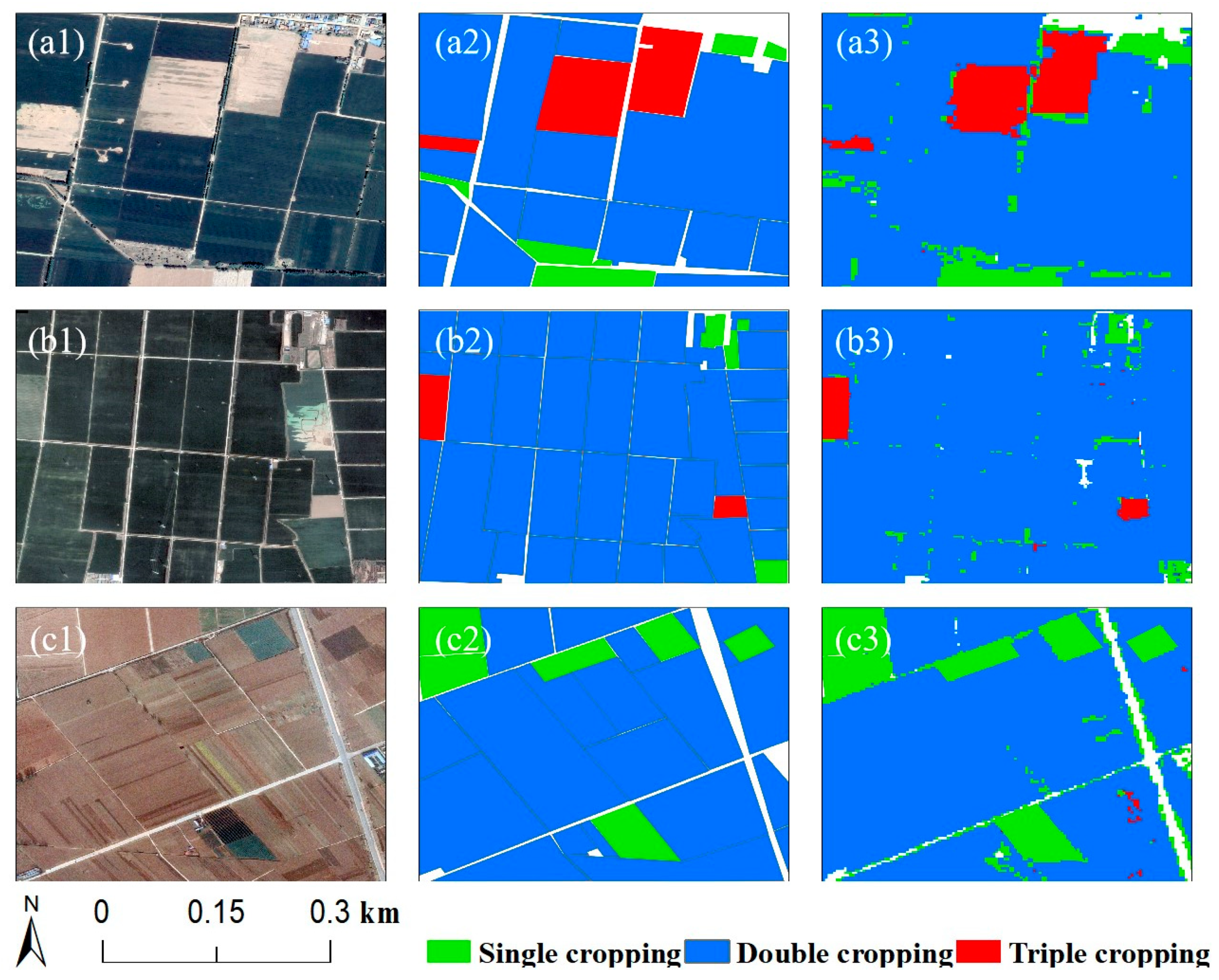
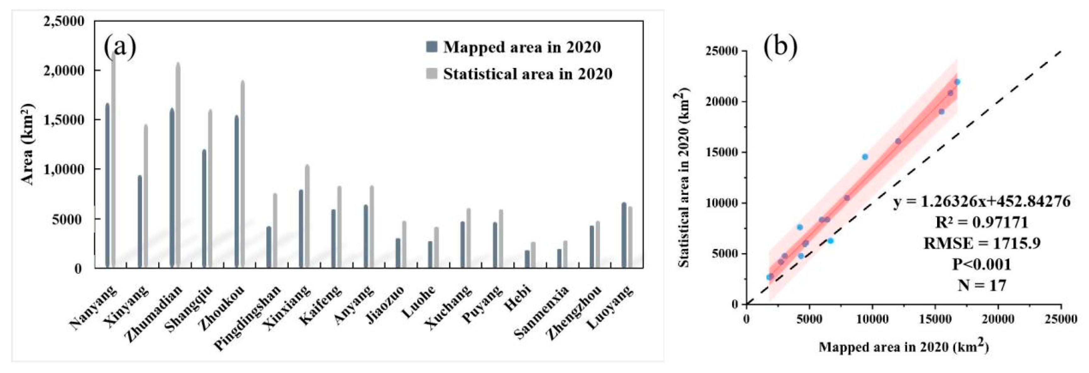
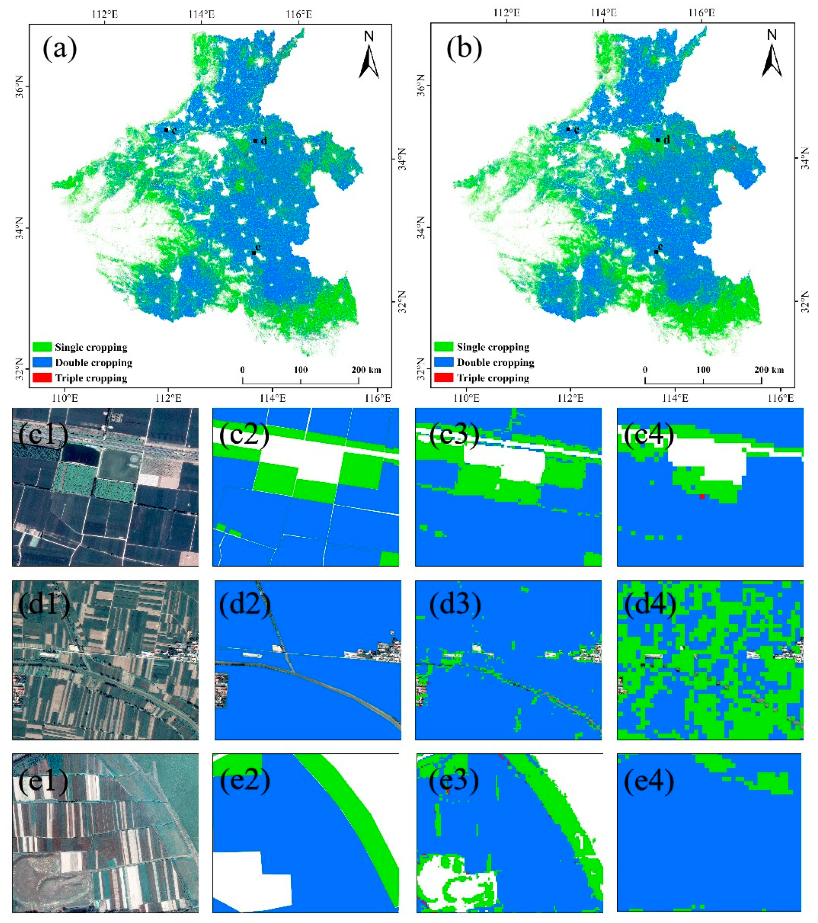
3.1. Annual Map of Crop Intensity in 2020

As described in Section 2.3.2, we determined the effective peak number of all cropland pixels in 2020 and drew a cropping intensity map with 10 m resolution in the Henan Province in 2020 (Figure 6). The planting systems in the Henan Province are dominated by single cropping (52,236.9 km²) and double cropping (74,334.1 km²), and the distribution of triple cropping is very small (1927.1 km²). A single cropland is mostly concentrated in the southern, western, and northwestern edges of the study area, accounting for 40.65% of the cropland in the Henan Province. Double cropland is mainly distributed in the central and eastern part of the study area, accounting for 57.85% of the cropland in the Henan Province. The distribution of triple cropland is scattered and irregular, mainly due to human influence (e.g., people’s preferences and needs), accounting for only 1.49% of the cropland in the Henan Province.

3.2. Accuracy Assessment

We used the validation samples set described in Section 2.2.2 to evaluate the accuracy of the cropping intensity map with 10 m spatial resolution in the Henan Province in 2020. Using the confusion matrix between the validation samples set and resultant map, we obtained that the OA and Kappa coefficient of the intensity map were 90.95% and 0.81, respectively (

Table 1. Accuracy assessment of cropping intensity classification in the study area.

Class	Error Matrix (Pixels)				Accuracy (%)
	Single	Double	Triple	Total	User’s	Producer’s	Overall	Kappa
Single	9448	1161	9	10,618	88.99	86.12	90.95	0.81
Double	1494	17,974	8	19,476	92.29	93.72
Triple	29	44	181	254	71.26	91.41
Total	10,971	19,179	198	30,348	/	/

). The UA of the single cropping system is greater than the PA, which indicates that the single cropping system is more likely to be omitted, resulting in the underestimation of the planting area of the single cropping system. At the same time, the PA of the double cropping system and triple cropping system is greater than that of UA, which indicates that the double cropping system and triple cropping system are more likely to be misclassified, leading to overestimation of the planting area of the double- and triple-cropping system.

Furthermore, we selected three areas with mixed planting systems. Each area is a square with a side length of 1 km. They were visually interpreted through ground reference data and generated polygons with different types of crop intensity. These polygons were used to evaluate the classification accuracy of our cropping intensity map quantitatively. Figure 7 intuitively describes the results of the accuracy assessment. Shrubs, roads, and houses are the main areas of misclassification. This is mainly because the side length of our pixel is 10 m, which is usually less than the width of the rural road. Overall, the consistency between our classification results and ground reference data is very obvious.

We also compared the crop statistics of cities (including 17 cities in total) in the Henan Province with our results (Figure 8). There is a significant linear relationship between the sown area derived from our results and the sown area derived from the statistical data (slope = 0.7692, R² = 0.9717, p < 0.001, RMSE = 1715.9 km²). The sown area was smaller in the cropping intensity maps than in the national statistical data for almost all cities, mainly because the cropland area was smaller in FROM-GLC10 than in the national statistical yearbook.

4. Discussion

4.1. Spatial Distribution of Cropping Intensity in Henan Province

The cropping intensity and crop types of cropland are not only affected by natural processes, but also by anthropogenic drivers [70]. The hydrothermal conditions in the south of the Henan Province are more abundant than those in the north. Therefore, in theory, the cropping intensity in the south should be higher than that in the north. However, our results indicate that most areas in the south (such as Xinyang City) are single cropping systems. The Xinyang area has sufficient rainfall, dense ponds, and high temperatures, which provide a good growth environment for rice growth. Through our field investigation, we found that the main factor affecting Xinyang’s planting system is the loss of population. As more and more young people migrate from rural to urban areas, the rural population of Xinyang has dropped sharply. Therefore, most cropland has changed from a double rice cropping system or triple rice cropping system to a single rice cropping system.

Different from the single rice cropping system in Xinyang, the cropping system in the mountainous areas around Nanyang is mainly single peanuts. This is because these areas have high terrain, poor soil quality, small cropland, and insufficient irrigation conditions. Therefore, farmers plant more drought-tolerant peanuts. In addition, the special growth characteristics of peanuts prevent it from being planted twice in the same area within a year, which is also the reason for the implementation of the single peanut cropping system in these areas. In Kaifeng City, the main cropping systems are wheat-peanut, garlic-corn, wheat-watermelon rotation. This is mainly because most of the cropland in Kaifeng City is sandy soil, with low soil water content and poor water retention capacity, which is suitable for planting drought-tolerant crops.

4.2. Algorithm Improvement

The peak point detection method has been widely used to map cropping intensity [31,32,49]. This method is simple and feasible, but it is more sensitive to noise in the time series. For example, the vegetation index time series of winter crops usually have two peaks in one growth cycle (Figure 5b). Therefore, it is necessary to use a supplementary algorithm to eliminate false peaks [5,71]. Gray et al. (2014) used the calendar-year thermal growth season to eliminate the extra peak of winter crops in autumn [32]. However, this method does not consider additional peaks caused by weather factors in other seasons. For example, summer crops may also have multiple peaks between April and October. Recently, Liu et al. (2020b) also used the peak point detection method to identify the peak of the crop growth curve, to extract the SOS and EOS on the crop growth curve, and finally map the cropping intensity of all seven typical grain production areas in China [46]. However, his algorithm has certain problems in identifying continuous peaks. Through our field investigation, we found that even the same crops in the same area have very different planting times. For example, in Kaifeng City, Henan Province, some garlic was planted in August of last year and harvested at the end of May of the next year, but a considerable part of garlic was planted in mid-September of last year and harvested in June of the next year. In Xinxiang City, Henan Province, some peanuts were sown in May and harvested in September, and some peanuts were sown at the end of March and harvested in August. Therefore, it is possible to identify continuous peaks only by limiting the NDVI trough from June to September. The length of the growth cycle is not limited by the sowing and harvesting time of crops. In this study, we not only used NDVI and LSWI time series to determine the potential growth cycle of the crop, but also further filtered the potential growth cycle according to the length of the crop growth cycle, which solves the problem of different sowing and harvest times in the same planting system in the Henan Province.

Moreover, the spatial resolution of 30 m is difficult to capture some small farmland and mixed agricultural landscapes (Figure 9). Higher spatial resolution of cropping intensity information not only helps decision makers to implement more accurate land management, but also helps to understand the dynamic changes of cropland under human influence [70]. In this study, we used Sentinel-2 images with a spatial resolution of 10 m to map cropping intensity in the Henan Province. Compared with previous studies using AVHRR (1000 m), MODIS (250 m to 1000 m), or Landsat (30 m) data, our results provide more spatial details (10 m) and successfully achieved fine mapping of large areas of complex planting areas. Higher resolution cropping intensity data can also improve the accuracy of many surface and crop models based on farmland planting systems [72,73,74].

4.3. Uncertainty

Although the method proposed in this study has successfully mapped fine (10 m) cropping intensity maps in complex planting areas, our analysis also pointed out several issues worthy of attention. Firstly, the accessibility of reliable cropland boundary data has always been a key constraint for cropland-based applications. In this study, we used the 10 m resolution global land cover product FROM-GLC10 [55] as the base cropland/non-cropland map. Although our research shows that the FROM-GLC10 product accurately represents the actual situation of cropland in the Henan Province, there are still certain classification errors, especially the rural roads and surrounding farmland in urban and rural residential areas (Figure 7). These errors are liable to be propagated to the final cropping intensity outputs. Meanwhile, the cropland data show the land cover in 2017, which may lead to a certain gap between our results (2020) and the actual cropland. With the release of the latest land use data, the cropland data synchronized with the study period can be used for more accurate remote sensing mapping in the future.

Secondly, in the process of constructing the time series, we used linear interpolation based on neighboring pixels to fill the blanks. If there is a lack of good-quality observation data when the peak (trough) is reached, then the real peak (trough) cannot be obtained by interpolation. In addition, due to cloud contamination, atmospheric variability, and bidirectional effects, noises appear in the NDVI time series. For these noises, we used the Maximum Value Composite (MVC) technique [75] and Savitzky–Golay filtering [76]. Figure 5 shows that the Savitzky–Golay filtering captures curve details and risk of underfitting. However, it is necessary to evaluate various smoothing methods (e.g., least-squares fits to asymmetric Gaussian functions [64] and double logistic functions [77], Whittaker smoother [78], wavelet transforms [79] and the best index slope extraction [80], etc.), which are expected to find more suitable methods to improve the accuracy of the results. Moreover, the microwave images from Sentinel-1 can easily pass through clouds, and can identify bare soil according to the degree of depolarization attained by the illuminated signal at the incident plane. In future research, remote sensing mapping can be combined with Sentinel-1A/B data not affected by weather.

Thirdly, the identification of the peak is also associated with assumptions that should be further verified. In some areas of Xinxiang City, the cropland near both sides of the road is usually a mixture of crops and evergreen trees. Since the LSWI of evergreen tree pixels always exceeds 0, the most mixed pixels of crops and evergreen trees are identified as single cropping. To exclude the extra peak of crops, our algorithm requires the length of each growth cycle to exceed 90 days. This threshold assumption, however, may be violated for special crops. For example, the growth period of lettuce and spinach is usually 20–40 days, so the growth cycle of these crops will be wrongly eliminated.

5. Conclusions

In this study, we developed a new phenological-based cropping intensity extraction method, and proposed a cropping intensity mapping system based on Sentinel-2A/B data. The system was used to map cropping intensity with 10 m resolution in the Henan Province in 2020. The overall accuracy is 90.95%, and the Kappa coefficient is 0.81. Compared with the cropping intensity map obtained from MODIS images, Landsat images, and images’ fusion of multi-source data in previous studies, the cropping intensity map in this study has more detailed spatial distribution and higher accuracy, and shows greater potential in estimating cropping intensity in complex planting areas. This dataset can provide quantitative information about the changes in the farming systems and improve our ability to predict grain yield.

References

1. Iizumi, T.; Ramankutty, N. How do weather and climate influence cropping area and intensity? Glob. Food Secur. 2015, 4, 46–50. [Google Scholar] [CrossRef] [Green Version]
2. Wu, W.; Yu, Q.; You, L.; Chen, K.; Tang, H.; Liu, J. Global cropping intensity gaps: Increasing food production without cropland expansion. Land Use Policy 2018, 76, 515–525. [Google Scholar] [CrossRef]
3. Thenkabail, P.; Lyon, J.G.; Turral, H.; Biradar, C. Remote Sensing of Global Croplands for Food Security; CRC Press: Boca Raton, FL, USA, 2009. [Google Scholar]
4. Shulan, J.; Lichun, H.; Lei, X. The relationship of multiple cropping index of arableland change and national food security in the middle and lower reaches of Yangtze River. Chin. Agric. Sci. Bull. 2011, 27, 208–212. [Google Scholar]
5. Yan, H.; Xiao, X.; Huang, H.; Liu, J.; Chen, J.; Bai, X. Multiple cropping intensity in China derived from agro-meteorological observations and MODIS data. Chin. Geogr. Sci. 2013, 24, 205–219. [Google Scholar] [CrossRef] [Green Version]
6. Lambin, E.F.; Meyfroidt, P. Global land use change, economic globalization, and the looming land scarcity. Proc. Natl. Acad. Sci. USA 2011, 108, 3465–3472. [Google Scholar] [CrossRef] [Green Version]
7. Yang, R.; Luo, X.; Xu, Q.; Zhang, X.; Wu, J. Measuring the Impact of the Multiple Cropping Index of Cultivated Land during Continuous and Rapid Rise of Urbani-zation in China: A Study from 2000 to 2015. Land 2021, 10, 491. [Google Scholar] [CrossRef]
8. Liu, L.; Xu, X.; Zhuang, D.; Chen, X.; Li, S. Changes in the Potential Multiple Cropping System in Response to Climate Change in China from 1960–2010. PLoS ONE 2013, 8, e80990. [Google Scholar] [CrossRef] [PubMed]
9. Wu, W.-B.; Yu, Q.; Peter, V.H.; You, L.-Z.; Yang, P.; Tang, H.-J. How Could Agricultural Land Systems Contribute to Raise Food Production Under Global Change? J. Integr. Agric. 2014, 13, 1432–1442. [Google Scholar] [CrossRef]
10. Zhang, J.; Feng, L.; Yao, F. Improved maize cultivated area estimation over a large scale combining MODIS–EVI time series data and crop phenological information. ISPRS J. Photogramm. Remote Sens. 2014, 94, 102–113. [Google Scholar] [CrossRef]
11. Sidike, P.; Sagan, V.; Maimaitijiang, M.; Maimaitiyiming, M.; Shakoor, N.; Burken, J.; Mockler, T.; Fritschi, F.B. dPEN: Deep Progressively Expanded Network for mapping heterogeneous agricultural landscape using WorldView-3 satellite imagery. Remote Sens. Environ. 2019, 221, 756–772. [Google Scholar] [CrossRef]
12. Zhao, W.; Li, A.; Nan, X.; Zhang, Z.; Lei, G. Postearthquake Landslides Mapping From Landsat-8 Data for the 2015 Nepal Earthquake Using a Pixel-Based Change Detection Method. IEEE J. Sel. Top. Appl. Earth Obs. Remote Sens. 2017, 10, 1758–1768. [Google Scholar] [CrossRef]
13. Arvor, D.; Dubreuil, V.; Simoes, M.; Bégué, A. Mapping and spatial analysis of the soybean agricultural frontier in Mato Grosso, Brazil, using remote sensing data. GeoJournal 2013, 78, 833–850. [Google Scholar] [CrossRef] [Green Version]
14. Chen, Y.; Lu, D.; Moran, E.; Batistella, M.; Dutra, L.V.; Sanches, I.D.; da Silva, R.F.B.; Huang, J.; Luiz, A.J.B.; de Oliveira, M.A.F. Mapping croplands, cropping patterns, and crop types using MODIS time-series data. Int. J. Appl. Earth Obs. Geoinf. 2018, 69, 133–147. [Google Scholar] [CrossRef]
15. Pan, L.; Xia, H.; Yang, J.; Niu, W.; Wang, R.; Song, H.; Guo, Y.; Qin, Y. Mapping cropping intensity in Huaihe basin using phenology algorithm, all Sentinel-2 and Landsat images in Google Earth Engine. Int. J. Appl. Earth Obs. Geoinf. 2021, 102, 102376. [Google Scholar] [CrossRef]
16. Biradar, C.M.; Xiao, X. Quantifying the area and spatial distribution of double- and triple-cropping croplands in India with multi-temporal MODIS imagery in 2005. Int. J. Remote Sens. 2011, 32, 367–386. [Google Scholar] [CrossRef]
17. Jain, M.; Mondal, P.; DeFries, R.S.; Small, C.; Galford, G. Mapping cropping intensity of smallholder farms: A comparison of methods using multiple sensors. Remote Sens. Environ. 2013, 134, 210–223. [Google Scholar] [CrossRef] [Green Version]
18. Fan, C.; Zheng, B.; Myint, S.W.; Aggarwal, R. Characterizing changes in cropping patterns using sequential Landsat imagery: An adaptive threshold approach and application to Phoenix, Arizona. Int. J. Remote Sens. 2014, 35, 7263–7278. [Google Scholar] [CrossRef]
19. Cao, F.; Tzortziou, M.; Hu, C.; Mannino, A.; Fichot, C.; Del Vecchio, R.; Najjar, R.G.; Novak, M. Remote sensing retrievals of colored dissolved organic matter and dissolved organic carbon dynamics in North American estuaries and their margins. Remote Sens. Environ. 2018, 205, 151–165. [Google Scholar] [CrossRef]
20. Adam, J.O.; Prasad, S.T.; Pardhasaradhi, T.; Xiong, J.; Murali, K.G.; Russell, G.C.; Kamini, Y. Mapping cropland extent of Southeast and Northeast Asia using multi-year time-series Landsat 30-m data using a random forest classifier on the Google Earth Engine Cloud. Int. J. Appl. Earth Obs. Geoinf. 2019, 81, 110–124. [Google Scholar] [CrossRef]
21. Xie, X.; Chen, J.M.; Gong, P.; Li, A. Spatial Scaling of Gross Primary Productivity Over Sixteen Mountainous Watersheds Using Vegetation Heterogeneity and Surface Topography. J. Geophys. Res. Biogeosciences 2021, 126, e2020JG005848. [Google Scholar] [CrossRef]
22. Li, J.; Roy, D.P. A Global Analysis of Sentinel-2A, Sentinel-2B and Landsat-8 Data Revisit Intervals and Implications for Terrestrial Monitoring. Remote Sens. 2017, 9, 902. [Google Scholar] [CrossRef] [Green Version]
23. Zhu, Z.; Woodcock, C.E. Continuous change detection and classification of land cover using all available Landsat data. Remote Sens. Environ. 2014, 144, 152–171. [Google Scholar] [CrossRef] [Green Version]
24. Yang, N.; Liu, D.; Feng, Q.; Xiong, Q.; Zhang, L.; Ren, T.; Zhao, Y.; Zhu, D.; Huang, J. Large-Scale Crop Mapping Based on Machine Learning and Parallel Computation with Grids. Remote Sens. 2019, 11, 1500. [Google Scholar] [CrossRef] [Green Version]
25. Xia, H.; Zhao, W.; Li, A.; Bian, J.; Zhang, Z. Subpixel Inundation Mapping Using Landsat-8 OLI and UAV Data for a Wetland Region on the Zoige Plateau, China. Remote Sens. 2017, 9, 31. [Google Scholar] [CrossRef] [Green Version]
26. Graesser, J.; Ramankutty, N. Detection of cropland field parcels from Landsat imagery. Remote Sens. Environ. 2017, 201, 165–180. [Google Scholar] [CrossRef] [Green Version]
27. Xu, W.; Sun, R.; Jin, Z. Extracting tea plantations based on ZY-3 satellite data. Trans. Chin. Soc. Agric. Eng. 2016, 32, 161–168. [Google Scholar]
28. Panigrahy, S.; Sharma, S. Mapping of crop rotation using multidate Indian Remote Sensing Satellite digital data. ISPRS J. Photogramm. Remote Sens. 1997, 52, 85–91. [Google Scholar] [CrossRef]
29. Zuo, L.; Dong, T.; Wang, X.; Zhao, X.; Yi, L. Multiple cropping index of Northern China based on MODIS/EVI. Trans. Chin. Soc. Agric. Eng. 2009, 25, 141–146. [Google Scholar]
30. Jiang, M.; Xin, L.; Li, X.; Tan, M.; Wang, R. Decreasing Rice Cropping Intensity in Southern China from 1990 to 2015. Remote Sens. 2019, 11, 35. [Google Scholar] [CrossRef] [Green Version]
31. Li, L.; Friedl, M.A.; Xin, Q.; Gray, J.; Pan, Y.; Frolking, S. Mapping Crop Cycles in China Using MODIS-EVI Time Series. Remote Sens. 2014, 6, 2473–2493. [Google Scholar] [CrossRef] [Green Version]
32. Gray, J.; Friedl, M.; Frolking, S.; Ramankutty, N.; Nelson, A.; Gumma, M.K. Mapping Asian Cropping Intensity With MODIS. IEEE J. Sel. Top. Appl. Earth Obs. Remote Sens. 2014, 7, 3373–3379. [Google Scholar] [CrossRef]
33. Hao, P.-Y.; Tang, H.-J.; Chen, Z.-X.; Yu, L.; Wu, M.-Q. High resolution crop intensity mapping using harmonized Landsat-8 and Sentinel-2 data. J. Integr. Agric. 2019, 18, 2883–2897. [Google Scholar] [CrossRef]
34. Ding, M.; Chen, Q.; Xiao, X.; Xin, L.; Zhang, G.; Li, L. Variation in Cropping Intensity in Northern China from 1982 to 2012 Based on GIMMS-NDVI Data. Sustainability 2016, 8, 1123. [Google Scholar] [CrossRef] [Green Version]
35. Wardlow, B.D.; Egbert, S.L.; Kastens, J.H. Analysis of time-series MODIS 250 m vegetation index data for crop classification in the U.S. Central Great Plains. Remote Sens. Environ. 2007, 108, 290–310. [Google Scholar] [CrossRef] [Green Version]
36. Galford, G.L.; Mustard, J.F.; Melillo, J.; Gendrin, A.; Cerri, C.C. Wavelet analysis of MODIS time series to detect expansion and intensification of row-crop agriculture in Brazil. Remote Sens. Environ. 2008, 112, 576–587. [Google Scholar] [CrossRef]
37. Sakamoto, T.; Yokozawa, M.; Toritani, H.; Shibayama, M.; Ishitsuka, N.; Ohno, H. A crop phenology detection method using time-series MODIS data. Remote Sens. Environ. 2005, 96, 366–374. [Google Scholar] [CrossRef]
38. Wang, J.; Xiao, X.; Liu, L.; Wu, X.; Qin, Y.; Steiner, J.L.; Dong, J. Mapping sugarcane plantation dynamics in Guangxi, China, by time series Sentinel-1, Sentinel-2 and Landsat images. Remote Sens. Environ. 2020, 247, 111951. [Google Scholar] [CrossRef]
39. Pan, L.; Xia, H.; Zhao, X.; Guo, Y.; Qin, Y. Mapping Winter Crops Using a Phenology Algorithm, Time-Series Sentinel-2 and Landsat-7/8 Images, and Google Earth Engine. Remote Sens. 2021, 13, 2510. [Google Scholar] [CrossRef]
40. Bargiel, D. A new method for crop classification combining time series of radar images and crop phenology information. Remote Sens. Environ. 2017, 198, 369–383. [Google Scholar] [CrossRef]
41. Xiang, M.; Yu, Q.; Wu, W. From multiple cropping index to multiple cropping frequency: Observing cropland use intensity at a finer scale. Ecol. Indic. 2019, 101, 892–903. [Google Scholar] [CrossRef]
42. Wang, C.; Fan, Q.; Li, Q.; SooHoo, W.M.; Lu, L. Energy crop mapping with enhanced TM/MODIS time series in the BCAP agricultural lands. ISPRS J. Photogramm. Remote Sens. 2017, 124, 133–143. [Google Scholar] [CrossRef] [Green Version]
43. Liu, J.; Zhu, W.; Atzberger, C.; Zhao, A.; Pan, Y.; Huang, X. A Phenology-Based Method to Map Cropping Patterns under a Wheat-Maize Rotation Using Remotely Sensed Time-Series Data. Remote Sens. 2018, 10, 1203. [Google Scholar] [CrossRef] [Green Version]
44. Qiu, B.; Luo, Y.; Tang, Z.; Chen, C.; Lu, D.; Huang, H.; Chen, Y.; Chen, N.; Xu, W. Winter wheat mapping combining variations before and after estimated heading dates. ISPRS J. Photogramm. Remote Sens. 2017, 123, 35–46. [Google Scholar] [CrossRef]
45. Zhao, Y.; Bai, L.; Feng, J.; Lin, X.; Wang, L.; Xu, L.; Ran, Q.; Wang, K. Spatial and Temporal Distribution of Multiple Cropping Indices in the North China Plain Using a Long Remote Sensing Data Time Series. Sensors 2016, 16, 557. [Google Scholar] [CrossRef] [PubMed] [Green Version]
46. Liu, L.; Xiao, X.; Qin, Y.; Wang, J.; Xu, X.; Hu, Y.; Qiao, Z. Mapping cropping intensity in China using time series Landsat and Sentinel-2 images and Google Earth Engine. Remote Sens. Environ. 2020, 239, 111624. [Google Scholar] [CrossRef]
47. Liu, C.; Zhang, Q.; Tao, S.; Qi, J.; Ding, M.; Guan, Q.; Wu, B.; Zhang, M.; Nabil, M.; Tian, F.; et al. A new framework to map fine resolution cropping intensity across the globe: Algorithm, validation, and implication. Remote Sens. Environ. 2020, 251, 112095. [Google Scholar] [CrossRef]
48. Qiu, B.; Zhong, M.; Tang, Z.; Wang, C. A new methodology to map double-cropping croplands based on continuous wavelet transform. Int. J. Appl. Earth Obs. Geoinf. 2014, 26, 97–104. [Google Scholar] [CrossRef]
49. Qiu, B.; Lu, D.; Tang, Z.; Song, D.; Zeng, Y.; Wang, Z.; Chen, C.; Chen, N.; Huang, H.; Xu, W. Mapping cropping intensity trends in China during 1982–2013. Appl. Geogr. 2017, 79, 212–222. [Google Scholar] [CrossRef]
50. Drusch, M.; Del Bello, U.; Carlier, S.; Colin, O.; Fernandez, V.; Gascon, F.; Hoersch, B.; Isola, C.; Laberinti, P.; Martimort, P.; et al. Sentinel-2: ESA’s optical high-resolution mission for GMES operational services. Remote Sens. Environ. 2012, 120, 25–36. [Google Scholar] [CrossRef]
51. Zhu, Z.; Woodcock, C.E. Object-based cloud and cloud shadow detection in Landsat imagery. Remote Sens. Environ. 2012, 118, 83–94. [Google Scholar] [CrossRef]
52. Huete, A.; Didan, K.; Miura, T.; Rodriguez, E.P.; Gao, X.; Ferreira, L.G. Overview of the radiometric and biophysical performance of the MODIS vegetation indices. Remote Sens. Environ. 2002, 83, 195–213. [Google Scholar] [CrossRef]
53. Zhang, Y.; Guindon, B.; Cihlar, J. An image transform to characterize and compensate for spatial variations in thin cloud contam-ination of Landsat images. Remote Sens. Environ. 2002, 82, 173–187. [Google Scholar] [CrossRef]
54. Zhu, Z.; Woodcock, C.E. Automated cloud, cloud shadow, and snow detection in multitemporal Landsat data: An algorithm de-signed specifically for monitoring land cover change. Remote Sens. Environ. 2014, 152, 217–234. [Google Scholar] [CrossRef]
55. Chen, B.; Xu, B.; Zhu, Z.; Yuan, C.; Suen, H.P.; Guo, J.; Xu, N.; Li, W.; Zhao, Y.; Yang, J.; et al. Stable classification with limited sample: Transferring a 30-m resolution sample set collected in 2015 to mapping 10-m resolution global land cover in 2017. Sci. Bull. 2019, 64, 370–373. [Google Scholar] [CrossRef] [Green Version]
56. Boles, S.H.; Xiao, X.; Liu, J.; Zhang, Q.; Munkhtuya, S.; Chen, S.; Ojima, D. Land cover characterization of Temperate East Asia using multi-temporal VEGETATION sensor data. Remote Sens. Environ. 2004, 90, 477–489. [Google Scholar] [CrossRef]
57. Chen, B.; Xiao, X.; Ye, H.; Ma, J.; Doughty, R.; Li, X.; Zhao, B.; Wu, Z.; Sun, R.; Dong, J.; et al. Mapping Forest and Their Spatial–Temporal Changes From 2007 to 2015 in Tropical Hainan Island by Integrating ALOS/ALOS-2 L-Band SAR and Landsat Optical Images. IEEE J. Sel. Top. Appl. Earth Obs. Remote Sens. 2018, 3, 852–867. [Google Scholar] [CrossRef]
58. Tucker, C.J. Red and photographic infrared linear combinations for monitoring vegetation. Remote Sens. Environ. 1979, 8, 127–150. [Google Scholar] [CrossRef] [Green Version]
59. Xiao, X.; Boles, S.; Liu, J.; Zhuang, D.; Frolking, S.; Li, C.; Salas, W.; Moore, B. Mapping paddy rice agriculture in southern China using multi-temporal MODIS images. Remote Sens. Environ. 2005, 95, 480–492. [Google Scholar] [CrossRef]
60. Running, S.W.; Loveland, T.R.; Pierce, L.L.; Nemani, R.; Hunt, E. A remote sensing based vegetation classification logic for global land cover analysis. Remote Sens. Environ. 1995, 51, 39–48. [Google Scholar] [CrossRef]
61. Griffiths, P.; Nendel, C.; Hostert, P. Intra-annual reflectance composites from Sentinel-2 and Landsat for national-scale crop and land cover mapping. Remote Sens. Environ. 2019, 220, 135–151. [Google Scholar] [CrossRef]
62. Xia, H.; Zhao, J.; Qin, Y.; Yang, J.; Cui, Y.; Song, H.; Ma, L.; Jin, N.; Meng, Q. Changes in Water Surface Area during 1989–2017 in the Huai River Basin using Landsat Data and Google Earth Engine. Remote Sens. 2019, 11, 1824. [Google Scholar] [CrossRef] [Green Version]
63. Kandasamy, S.; Baret, F.; Verger, A.; Neveux, P.; Weiss, M. A comparison of methods for smoothing and gap filling time series of remote sensing observations—Application to MODIS LAI products. Biogeosciences 2013, 10, 4055–4071. [Google Scholar] [CrossRef] [Green Version]
64. Jönsson, P.; Eklundh, L. Seasonality extraction by function fitting to time-series of satellite sensor data. IEEE Trans. Geosci. Remote Sens. 2002, 40, 1824–1832. [Google Scholar] [CrossRef]
65. Dong, J.; Xiao, X.; Kou, W.; Qin, Y.; Zhang, G.; Li, L.; Jin, C.; Zhou, Y.; Wang, J.; Biradar, C.; et al. Tracking the dynamics of paddy rice planting area in 1986–2010 through time series Landsat images and phenology-based algorithms. Remote Sens. Environ. 2015, 160, 99–113. [Google Scholar] [CrossRef]
66. Waha, K.; Dietrich, J.P.; Portmann, F.T.; Siebert, S.; Thornton, P.K.; Bondeau, A.; Herrero, M. Multiple cropping systems of the world and the potential for increasing cropping intensity. Glob. Environ. Chang. 2020, 64, 102131. [Google Scholar] [CrossRef] [PubMed]
67. Xunhao, L. Farming System and Farming System Regional Planning in China. J. China Agric. Resour. Reg. Plan. 2002, 5, 11–15. [Google Scholar]
68. Sobrino, J.; Raissouni, N.; Li, Z.-L. A comparative study of land surface emissivity retrieval from NOAA data. Remote Sens. Environ. 2001, 75, 256–266. [Google Scholar] [CrossRef]
69. Olofsson, P.; Foody, G.M.; Herold, M.; Stehman, S.V.; Woodcock, C.E.; Wulder, M.A. Good practices for estimating area and assessing accuracy of land change. Remote Sens. Environ. 2014, 148, 42–57. [Google Scholar] [CrossRef]
70. Belgiu, M.; Csillik, O. Sentinel-2 cropland mapping using pixel-based and object-based time-weighted dynamic time warping anal-ysis. Remote Sens. Environ. 2018, 204, 509–523. [Google Scholar] [CrossRef]
71. Yan, H.; Liu, F.; Qin, Y.; Niu, Z.; Doughty, R.; Xiao, X. Tracking the spatio-temporal change of cropping intensity in China during 2000–2015. Environ. Res. Lett. 2018, 14, 035008. [Google Scholar] [CrossRef]
72. Xie, X.; Li, A. An Adjusted Two-Leaf Light Use Efficiency Model for Improving GPP Simulations Over Mountainous Areas. J. Geophys. Res. Atmos. 2020, 125, e2019JD031702. [Google Scholar] [CrossRef]
73. Xie, X.; Li, A. Development of a topographic-corrected temperature and greenness model (TG) for improving GPP estimation over mountainous areas. Agric. For. Meteorol. 2020, 295, 108193. [Google Scholar] [CrossRef]
74. Zhao, W.; Li, A. A Review on Land Surface Processes Modelling over Complex Terrain. Adv. Meteorol. 2015, 2015, 1–17. [Google Scholar] [CrossRef] [Green Version]
75. Holben, B.N. Characteristics of maximum-value composite images from temporal AVHRR data. Int. J. Remote Sens. 1986, 7, 1417–1434. [Google Scholar] [CrossRef]
76. Chen, J.; Jönsson, P.; Tamura, M.; Gu, Z.; Matsushita, B.; Eklundh, L. A simple method for reconstructing a high-quality NDVI time-series data set based on the Savitzky–Golay filter. Remote Sens. Environ. 2004, 91, 332–344. [Google Scholar] [CrossRef]
77. Beck, P.S.; Atzberger, C.; Høgda, K.A.; Johansen, B.; Skidmore, A. Improved monitoring of vegetation dynamics at very high latitudes: A new method using MODIS NDVI. Remote Sens. Environ. 2006, 100, 321–334. [Google Scholar] [CrossRef]
78. Atzberger, C.; Eilers, P.H.C. Evaluating the effectiveness of smoothing algorithms in the absence of ground reference measurements. Int. J. Remote Sens. 2011, 32, 3689–3709. [Google Scholar] [CrossRef]
79. Campos, A.N.; Di Bella, C.M. Multi-Temporal Analysis of Remotely Sensed Information Using Wavelets. J. Geogr. Inf. Syst. 2012, 4, 383–391. [Google Scholar] [CrossRef] [Green Version]
80. Viovy, N.; Arino, O.; Belward, A.S. The Best Index Slope Extraction (BISE): A method for reducing noise in NDVI time-series. Int. J. Remote Sens. 1992, 13, 1585–1590. [Google Scholar] [CrossRef]
Figure 1. (a) Location and (b) Spatial pattern of the land type of Henan Province, PRC.
Ijgi 10 00587 g001
Figure 2. (a,b) Numbers of total observations and good-quality observations for individual pixels during the study period, respectively. (c) Number of Sentinel-2A/B images per month during 1 July 2019–1 July 2021. (d) Average number of total and good-quality observations per pixel during 1 July 2019–1 July 2021.
Ijgi 10 00587 g002
Figure 3. (a) is the spatial distribution of sample points. (b1d1) are samples of different cropping intensities. (b2d2) areas generated by the samples. (b1) and (b2), (c1) and (c2), (d1) and (d2) correspond to b, c, d in (a), respectively. Image source: Image 2021 Maxar Technologies and 2021 CNES/Airbus. Image date: Identified in the picture. Color composite: RGB (red, green, blue).
Ijgi 10 00587 g003
Figure 4. Flowchart of the overall approach for mapping the cropping intensity.
Ijgi 10 00587 g004
Figure 5. Temporal profile of NDVI and LSWI indices for cropping intensity sample sites with (a) single cropping (114.7136° E, 32.0998° N), (b) double cropping (115.0976° E, 34.1655° N), (c) double cropping (114.7069° E, 32.4664° N), and (d) triple cropping (115.2695° E, 33.8918° N).
Ijgi 10 00587 g005
Figure 6. (a) Cropping intensity map with 10 m spatial resolution in Henan Province in 2020. (b1d1) are zoom-in views of three randomly selected areas; (b2d2) are the landscapes from Google Earth images. (b1) and (b2), (c1) and (c2), (d1) and (d2) correspond to b, c, d in (a), respectively. Image source: Image 2021 Maxar Technologies and 2021 CNES/Airbus. Image date: Identified in the picture. Color composite: RGB (red, green, blue).
Ijgi 10 00587 g006
Figure 7. Accuracy evaluation of the results of cropping intensity classification based on the composite image of the study area. (a1c1) are Google Earth images; (a2c2) are ground reference data generated by visual interpretation combined with survey data; (a3c3) are results in this study. Image source: Image 2021 CNES/Airbus. Color composite: RGB (red, green, blue).
Ijgi 10 00587 g007
Figure 8. (a) A comparison of sown area estimates by city between the cropping intensity map in 2020 and the agricultural statistical data reported for 2020. (b) The black dotted line is the y = x line, and the red area represents the 95% confidence interval and prediction zone.
Ijgi 10 00587 g008
Figure 9. (a) Classification results of this paper. (b) Liu et al. (2020b) classification results. (c1e1) Google Earth image. (c2e2) Reference data by visual interpretation based on Google Earth image. (c3e3) Classification results of this paper. (c4e4) Liu et al. (2020b) classification results. Image source: Image 2021 CNES/Airbus. Color composite: RGB (red, green, blue).
Ijgi 10 00587 g009