Reconstruction of Multi-Temporal Satellite Imagery by Coupling Variational Segmentation and Radiometric Analysis

Abstract

Digital images, and in particular satellite images acquired by different sensors, may present defects due to many causes. Since 2013, the Landsat 7 mission has been affected by a well-known issue related to the malfunctioning of the Scan Line Corrector producing very characteristic strips of missing data in the imagery bands. Within the vast and interdisciplinary image reconstruction application field, many works have been presented in the last few decades to tackle the specific Landsat 7 gap-filling problem. This work proposes another contribution in this field presenting an original procedure based on a variational image segmentation model coupled with radiometric analysis to reconstruct damaged images acquired in a multi-temporal scenario, typical in satellite remote sensing. The key idea is to exploit some specific features of the Mumford–Shah variational model for image segmentation in order to ease the detection of homogeneous regions which will then be used to form a set of coherent data necessary for the radiometric reconstruction of damaged regions. Two reconstruction approaches are presented and applied to SLC-off Landsat 7 data. One approach is based on the well-known histogram matching transformation, the other approach is based on eigendecomposition of the bands covariance matrix and on the sampling from Gaussian distributions. The performance of the procedure is assessed by application to artificially damaged images for self-validation testing. Both of the proposed reconstruction approaches had led to remarkable results. An application to very high resolution WorldView-3 data shows how the procedure based on variational segmentation allows an effective reconstruction of images presenting a great level of geometric complexity.

1. Introduction

Digital imaging is becoming increasingly common and is now being used in a growing variety of fields spanning from computer vision to medical imaging and remote sensing, just to mention a few. Due to various causes, be they technological or natural, images may often contain radiometric distortions or partial lack of information. The need to recover lost or distorted information led to important development of image restoration and reconstruction algorithms.

This work presents a new approach to image reconstruction based on the coupling of an image segmentation variational model and the radiometric analysis of multi-temporal satellite imagery. The reconstruction of satellite imagery is crucial to improve the performance of further image processing tasks such as classification, spectral unmixing, and object detection.

Among the many past and active satellite missions for Earth Observation (EO) purposes, the Landsat 7 mission presents a specific data-loss issue that attracted and still attracts a lot of interest in the image reconstruction field. The Landsat 7 mission, operative since 1999 within the NASA’s ESE (Earth Science Enterprise) program, exploits the Enhanced Thematic Mapper Plus (ETM+) sensor. The ETM+ sensors cover visible red, green, and blue (RGB), Near-InfraRed (NIR), Short-Wave InfraRed (SWIR), Mid-InfraRed (MIR), and Thermal InfraRed (TIR) spectral bands with a 8-bit radiometric resolution (transmitted) and spatial resolutions of 30, 60, and 15 m for RGB/NIR/SWIR/MIR, TIR, and panchromatic bands, respectively. Imagery bands are acquired with a repeat cycle of 16 days. The science mission will continue until mid-2021 (https://www.usgs.gov/news/successful-maneuver-spells-beginning-end-landsat-7).

On 31 May 2003, the Scan Line Corrector (SLC), the on-board instrument that manages the direction of the scan line in order to compensate for the forward satellite movement during scanning, encountered a permanent failure. From that date, Landsat 7 scenes are called SLC-off. Without SLC, the line of sight of the instrument cannot make the correct U-turn at the end of the scan line, tracing instead a zig-zag pattern. This results in scenes partly being scanned twice and partly not being scanned at all. The data-loss due to SLC failure does not affect the segment in the central 22 km of the captured scene, but produces instead cross-track data-loss stripes, swelling from the center of the image to its edges. SLC-off images lack about 22% of the data, and the maximum width of the data gap is about 15 pixels, corresponding to about 450 m of data loss at the edges. SLC-off stripes are not located exactly in the same position in different scenes, and also in the same scene they can be misaligned by one pixel between different bands, which is the cause of the clearly visible dark red, yellow, and green pixels and the edges of the SLC-off bands.

Research in satellite image restoration received a boost especially since Landsat 7 Scan Line Corrector failure, an event that left a critical and permanent degradation in one of the most important remote sensing missions. Even thought Landsat 8 was launched on 11 February 2013, its predecessor is still functioning and a ten-year period of damaged images ought to be recovered.

As a matter of fact, a plethora of different reconstruction algorithms were presented, each with its own peculiar characteristics that highlight the similarities and differences between them [1,2,3,4,5,6,7,8,9,10].

On a general basis, image reconstruction algorithms can be distinguished into two main classes:

• single-image reconstruction;
• multi-image reconstruction

Single-image reconstruction algorithms are mainly applied in medical imaging and computer vision fields, whereas multi-image reconstruction algorithms are better suited for multi-temporal or multi-source applications in satellites for the image processing field. In the following pages, a damaged or corrupted image will be called target image and an image from which any kind of information is derived for the reconstruction of the damaged regions of a target image will be called base image.

Approaches to the multi-image reconstruction problem can be classified as:

• compositing approach: filling data gaps in target image directly with values from other base images, sometimes rescaled using a linear transformation based on global mean values of base and target images;
• nearest-neighbor approach: making use of values in pixels near the one to be inpainted in order to obtain statistics of a reference data-pool from which the reconstructed values are calculated;
• geostatistics approach: using kriging to explicitly take into account spatial correlation to predict reconstructed values and estimation errors;
• segmentation approach: identifying clusters of homogeneous pixels automatically to build reference data-pools from which statistics for calculation of values to be reconstructed are extracted.

The original solution presented in this work exploits only geometric and radiometric information derived from target and base images acquired in a multi-temporal scenario and does not rely on other externals of ancillary information, such as land cover maps. The proposed procedure permits the reconstruction of complex geometric features, even when completely damaged, under the reasonable hypothesis that in the time span between the acquisition epochs of target and base images such features did not undergo significant modifications. The procedure exploits an image segmentation variational model proposed by Mumford and Shah [11] which eases the identification of coherent regions within a segmented image followed by radiometric analysis of correspondent coherent regions detected on target and base images. Intuitively, the main advantage of the Mumford–Shah variational model is that the image undergoes a smoothing process that respects discontinuities in the image. For this reason, on the one hand, the radiometric variability of segmented regions is reduced because of noise reduction associated with the smoothing process, and, on the other hand, the geometric quality of segmented regions is not compromised by the same smoothing process because its action is automatically suppressed on the region boundaries. As a consequence, segmented regions of high quality led to an improved identification of coherent regions. Two different approaches for radiometric analyses are considered for reconstruction: the first approach is based on the Histogram Matching (HM) transformation and the second one is based on the eigendecomposition (ED) of the covariance matrix of a set of imagery bands and on sampling of Gaussian distributions. The entire procedure was implemented using free and open source software and by means of original programs. Segmentation and detection of coherent regions were carried out using GRASS GIS while radiometric analyses and reconstructions were implemented by means of Python code and the PyGRASS Application Programming Interface (API) [12]. The proposed procedure was applied to synthetically damaged imagery for self-validation purposes. WorldView-3 and Landsat 7 bands were processed, using different values of variational model parameters, the quality of reconstructed bands was statistically assessed using original not-damaged imagery as reference information. Results for Landsat 7 8-bit Digital Numbers (DNs) show error means around ${10}^{-2}$ with standard deviation of a few units of intensity (error variances in the range $({10}^0,{10}^1$) and $R^2$ coefficient of determination very close to 1, see Tables 2 and 4. Applications to real-damaged Landsat 7 confirm the quality of the reconstructions obtained by the application of the methodology, see Figures 19 and 20.

The content of the manuscript is the following: some existing algorithms for satellite imagery reconstruction are introduced in Section 2; a brief presentation of the Mumford–Shah variational model for image segmentation and its analytical aspects is given in Section 3; the proposed methodology is detailed in Section 4; results of application of the procedure to WorldView-3 and Landsat 7 data are presented in Section 5 and discussed in Section 6 along with open problems and perspectives.

2. Overview of Selected Standard Algorithms

2.1. Histogram Matching Methods

Histogram matching consists of transforming the values of a data set by aligning the empirical cumulative distribution function (ECDF) of the data set to the ECDF of another data set; it is widely used in different fields of image processing. Scaramuzza et al. [13] proposed a first algorithm to tackle the Landsat 7 SLC-off problem; the algorithm was later assumed as a Phase 1 methodology by USGS in order to produce Landsat 7 SLC gap-filled products. The algorithm consists of mapping which pixels in an SLC-off image are valid and which have to be filled, creating a gap mask for each band. A linear relation between a base scene and the target scene is identified and used to transform the target histogram. The identification of the model parameter is computationally expensive and therefore replaced by the so-called method of moments to estimate gain and bias values on the basis of mean and standard deviation of the two data sets. This latter method, once applied to the whole images, is known as Global Linear Histogram Matching (GLHM). The method performs well on homogeneous scenes, it is not effective on scenes of heterogeneous landscapes, and useless on scenes with snow or clouds. For these reasons, GLHM was substituted by a Local Linear Histogram Matching (LLHM) model in which gain and bias are calculated only from those values in a moving window. This algorithm performs generally well and requires very little computational effort, but creates some striping or shading around sharp edges or abrupt land cover changes. The Phase 1 algorithm was further enhanced and updated by USGS [14] and hence officially adopted as a Phase 2 methodology. The enhancement allows for the use of a set of base scenes instead of just one. After defining a preference order in the available base images, the LLHM algorithm is applied to the smallest window containing a minimum number of valid pixels in both base and target data. Other enhancements are made in order to correct unreasonable gains and outliers, mitigating the effect of clouds and snow. Results of the Phase 2 algorithm are sensitive to the order of the base images, and all these enhancements lead in any case to poor results in scenes characterized by sun glint, snow, clouds, or high heterogeneity, and especially in scenes consisting of numerous small features. Aghamohamadnia and Abedini [15] proposed an improved algorithm aimed at enhancing the results of moving neighbor selection algorithms by coupling them with a morphology selection scheme. In the first step, the LLHM method is used to mask the SLC-off stripes, then a morphological operator is exploited to extract the outer pixels of SLC-off stripes. For each pixel, a stitch line is then created using an algorithm that searches for the most radiometrically similar pixels from either filled or non-filled adjacent pixels groups. The stitch lines can be extended iterating this procedure using the newly found pixels as center points. The borderline pixels are then updated using a local weighted mean. The whole method can be iterated considering the updated values as non-filled, and then updating the inner pixels of stitch lines. This method was proven useful for improving the result of any method smoothing edges of different land cover areas even if, it being based on mean estimators, filled stripe’s borders result smoothed out.

2.2. Neighborhood Similar Pixel Interpolation Method

The Neighborhood Similar Pixel Interpolation (NSPI) method, proposed by Chen et al. [7], is based on the assumption that pixels of the same land cover, within a determined neighborhood of a pixel to be restored, present similar spectral features and temporal patterns. The basic assumption of NSPI is that no significant large scale land cover change applies between the acquisition of a base and a target image. Firstly, outside the gaps common pixels are selected in both the base and target images, then the search for similar neighboring pixels is operated on the base image with an adaptive moving window based searching procedure. After the evaluation of a given measure of spectral similarity of the neighbor pixels within the moving window, the value of the target pixel is estimated in all bands, applying a weighted mean based on the similarity measure and on the Euclidean distance of each valid pixel from the target pixel. Two different methods are then used to estimate the value of a target pixel. The first method is based on a weighted mean of radiometrically similar neighbor pixels while the second tries to take into account the temporal variation of the target pixels, using the calculated weights to estimate the change of pixel values that occurred between two acquisition epochs. The accuracy of the two methods depends on the heterogeneity of the observed areas: the first method should be used for images with relative homogeneity and slow temporal change, the second method is more suitable for images with heterogeneous regions. A combination of the two methods is also feasible and aimed at finding a compromise between synchronous spatial homogeneity and diachronic evolution. The NSPI method performs generally better than LLHM, in particular for large temporal intervals between base and target images.

2.3. Geostatistical Method

Zhang et al. [16] proposed to use a geostatistical technique to exploit spatial correlation for the reconstruction of missing values in a damaged image. Geostatistical kriging models are interpolation algorithms providing unbiased estimations with minimum error variance. Spatial correlation is described by means of specific models fitting the so-called empirical semivariograms. The least squares method is involved in the estimation of the parameters of the model adopted to predict the value of the modeled variable in a specific location. In satellite imagery gap-filling algorithms, different geostatistics techniques can be considered, in particular, single variable models can be used when a base image is not at hand, whereas multiple variable models can be adopted to gain statistical information from a non-corrupted base image as done in Direct Sampling methods (e.g., [17]). In general, kriging techniques are used to interpolate the variable values at arbitrary locations. In the specific case of SLC-off data loss, the gaps have a peculiar pattern, and this ensures that the model parameters need to be estimated only once for each pattern, so that computational time is drastically reduced. Moreover, a normal score transformation is commonly applied to reduce negative impacts of strong skewness in the data set. Compared to the LLHM model, results of kriging based approaches present reduced striping and visual artifacts almost everywhere except on boundaries between different land covers. In general, kriging models predict data with less spatial variability than that of observed data, so, while analyzing reconstructed stripes, a stronger homogeneity can be noticed and the reconstruction of different land cover regions and boundaries is not easily achievable. Moreover, kriging models are usually applied to one band at time excluding the possibility to take into account the possibly relevant band covariance.

3. Mumford–Shah Variational Model for Image Segmentation

Mumford and Shah (1989) proposed to tackle the segmentation problem in computer science by finding a decomposition $R=R_1\cup R_2\cup \cdots \cup R_n$ of an input data g given in a two-dimensional domain $\Omega$ by means of the minimization of a functional depending on a piece-wise smooth approximation u of g. The approximating function varies smoothly within each $R_i$, and it is allowed to be discontinuous over a measurable one-dimensional set K of curves, e.g., the boundaries of the elements of R but not strictly only those.

The MS segmentation is achieved by the minimization of the functional:

$$\begin{array}{cc}\hfill \mathcal{MS}(u,K)& :={\int }_{\Omega }{|u-g|}^{2}dx+\lambda {\int }_{\Omega \setminus K}{|\nabla u|}^{2}dx+\alpha \mathcal{H}(K\cap \Omega ),\hfill \end{array}$$

(1)

where: $u\in C^1(\Omega \setminus K)$ and $\mathcal{H}$ is the 1-dimensional Hausdorff measure.

The parameters $\lambda$ and $\alpha$ act as weights balancing contributions of the three terms of the Mumford–Shah functional; the roles of the three terms being:

to keep u as close as possible to g;

to keep u as smooth as possible everywhere but over K;

to keep the length of the discontinuity set of u as short as possible,

where the last action is required to avoid trivial over-segmented solutions.

The Mumford–Shah functional Equation (1) represents a classical example of so-called free discontinuity problems as introduced by De Giorgi [18] and nowadays widely adopted also in one-dimension signal processing and in three-dimensional domains such as those involved in fracture analysis.

Despite its clear structure, analytical results for the Mumford–Shah functional (1) are very difficult to obtain because both surface and line energies are involved and because the support of the line energy depends on an unknown set.

After [19], Ambrosio et al. [20] and Modica and Mortola [21] proposed an equivalent relaxed functional was proposed, which is analytically solvable and simpler from a computational point of view. In short, a different class of approximating functions is considered so that the new functional no longer depends on the unknown set k. Moreover, an auxiliary two-dimensional function s is introduced whose integral converges to the length of the one-dimensional, discontinuity set $S_u$ of the approximating function. In this way, the new functional depends only on the approximating function u and involves only surface energies:

$$\begin{array}{c}\hfill {\mathcal{F}}_{ϵ}(u,s):={\int }_{\Omega }{|u-g|}^2+\lambda s^2{|\nabla u|}^2+\alpha \left[{ϵ|\nabla s|}^2+\frac{1}{4ϵ}{(s-1)}^2\right]dx,\end{array}$$

(2)

where now u belongs to the space of Special Functions of Bounded Variation $SBV(\Omega )$ [20], $ϵ$ is the convergence parameter, $s:\Omega \to [0,1]$ approximates the indicator function of the discontinuity set $S_u$, and it is equal to 0 on $S_u$ and 1 elsewhere.

From a practical point of view, $\lambda$ can be seen as a scale parameter controlling the smoothness of the solution. The larger the value of $\lambda$, the more the approximating function is close to a piece-wise constant solution. The parameter $\alpha$ instead can be seen as a noise sensitivity parameter which influences the discontinuity detection process; for $\alpha$ values close to 0, a high number of small segmented regions, and hence many discontinuities, are found.

More information about analytical and numerical aspects of Mumford–Shah functional and its implementation can be found in [22].

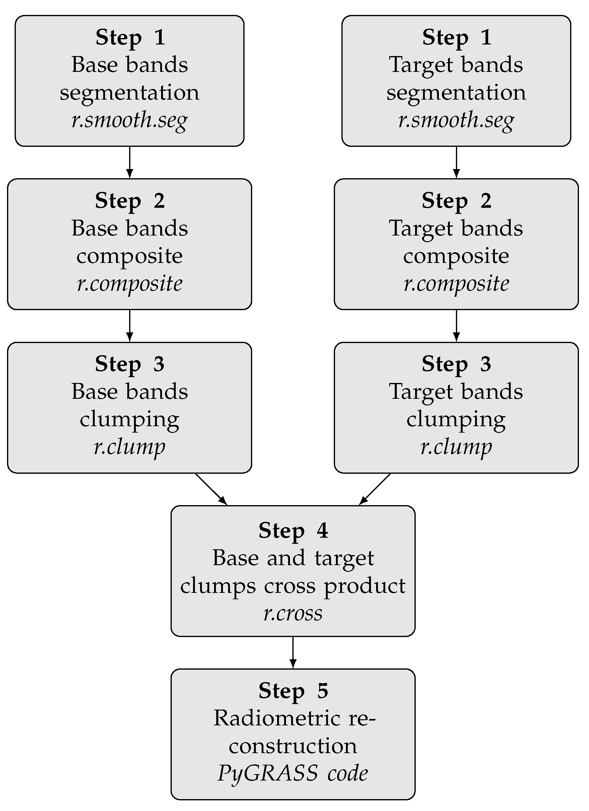
4. Coupling Variational Segmentation and Radiometric Analysis for Multi-Temporal Images Reconstruction

The proposed procedure consists of a set of steps to be applied in a sequential order:

• variational segmentation of base and target imagery bands;
• composition of integer rounded segmented bands;
• identification and labeling of connected components (clumps) of composite values;
• calculation of cross product of base and target clump labels;
• radiometric reconstruction.

A flowchart of the proposed procedure is shown in Figure 1; every step is detailed hereafter.

Step 1

Mumford–Shah variational segmentation is applied to base and target imagery bands at hand. In this work, the processing was carried out on digital numbers. A unique mask of SLC-off stripes is used for the processing of target bands. The values of model parameters $\alpha$ and $\lambda$ are selected on an empirical base after a few test; when working with Landsat 7 and DNs, one can start with $\alpha =500$ and $\lambda =8$. The same parameter values were used in the processing bands of each single scene, either base or target. Parameter values different between scenes, i.e., acquisition epochs, are conveniently selected to take into account inter-epochs radiometric differences. To verify if different parameter values yield consistent inter-epoch results, i.e., segmented regions of comparable dimension and shape, segmented base and target bands can be either visually or automatically compared. At this stage, the choice of very different parameter values may depend on very high radiometric differences between base and target bands suggesting the need to look for better base imagery to ease the radiometric reconstruction of the damaged target regions. The Mumford–Shah variational segmentation outputs a real valued piece-wise smooth approximation. Segmented values are rounded to restore integer consistency with input DN. Rounding introduces minor changes with respect to typical DN variances in satellite imagery and much less than the amount of noise-reduction that occurred in segmented regions.

Step 2

Composition of integer segmented bands is an easy way to classify the outputs of the previous step. In practice, a total of 32 intensity levels per band are used in the composition, resulting in a 15 bit composed image with 32,768 possible values when, for example, the composition of three bands is performed.

Step 3

Dealing with integer composed imagery greatly simplifies the identification and labeling of connected components. Otherwise, if real values were processed, a threshold based fuzzy clumping or an even more sophisticated classification algorithm would be necessary to identify and label segmented regions in a suitable way.

Step 4

The cross product of base and target clump labels produces all possible combinations of inter-scene clump labels. Each combination found is associated with the values of the base and target clump labels, allowing for returning to the original integer segmentation values.

The output of this step serves as a basic information layer for the reconstruction step. The SLC-off strips mask permits to separate regions to be reconstructed from those from which radiometric analysis will be conducted.

For each clump following within the regions to be reconstructed, the reconstruction data set is made of all the pixels belonging to every non-corrupted base clump that shares the same intensity level in the base composite map.

Given the value of the intensity level in the base composite map, it is possible to go back to the original integer segmentation values to be used as a data set for radiometric reconstruction.

If no identical intensity level can be found, the reconstruction database consists of all clumps with an intensity level as close as possible to the input intensity level. The distance measure is the Euclidean distance in the integer segmented band space and a threshold-based proximity criterion adopted to build the reconstruction database.

Step 5

Two different criteria were considered for the final radiometric reconstruction.

The first approach is based on the HM transformation. The ECDFs of base and target images are computed considering only non-corrupted regions and the parameters of the HM transformation are estimated. For each pixel to be reconstructed, its value in the base image $x_b$ is read and its cumulative frequency value $F_b\left(x_b\right)$ is evaluated. The reconstructed value in the target image ${\widehat{x}}_t$ is the one that holds the equality $F_t\left({\widehat{x}}_t\right)=F_b\left(x_b\right)$.

The second approach is based on ED and Gaussian distribution sampling. For base homogeneous regions, the band covariance matrix is computed. The data set is transformed according to ED to permit statistical sampling from uncorrelated Gaussian distributions with known mean and variance. The sampling is drawn once for each pixel to be reconstructed. For the sets of base non-corrupted regions with a total count below 30 units, ED and Gaussian sampling are not performed and reconstructed values are set to the mean value of the set of base non-corrupted regions.

The procedure was developed considering the processing of DNs. Performing radiometric reconstruction of DNs permits to deal with satellite detectors raw observations before other standard processing is performed. Moreover, dealing with integer quantities opens the possibility to effectively use simple tools, such as band composition and connected component analysis, for forming coherent homogeneous regions to be used in the statistically based radiometric reconstruction approaches which run at the target image level. In fact, when the HM approach is involved, the matching of the histograms is based on the correspondent of base and target clumps, and also, when the ED approach is involved, the statistics analysis for the reconstruction is actually performed at the target level as well. Nevertheless, the procedure can be easily adapted for processing both Top Of Atmosphere (TOA) and Bottom Of Atmosphere (BOA) physical quantities derived from DN values. In these cases, a more sophisticated classification method should be used to produce clumps because of the float nature of reflectance/radiance values. Once the clumps are at hand, the following steps of the procedure remain unaffected by the reduction of DNs to physical quantities as it is for their initial variational segmentation.

5. Results

5.1. Applications for Self-Validation

Some applications were conducted to verify the procedure implementation and to assess the procedure performance in the absence of radiometric alterations in a self-validation scenario. For that, in each of the following applications, base images were artificially corrupted to produce synthetic target images. Many self-validation tests were conducted, varying band combinations, ($\alpha$, $\lambda$) parameters and using both ED and HM based reconstruction methods. In the following sections, results of two self-validation tests are described. Application to a real case is presented later in the dedicated section.

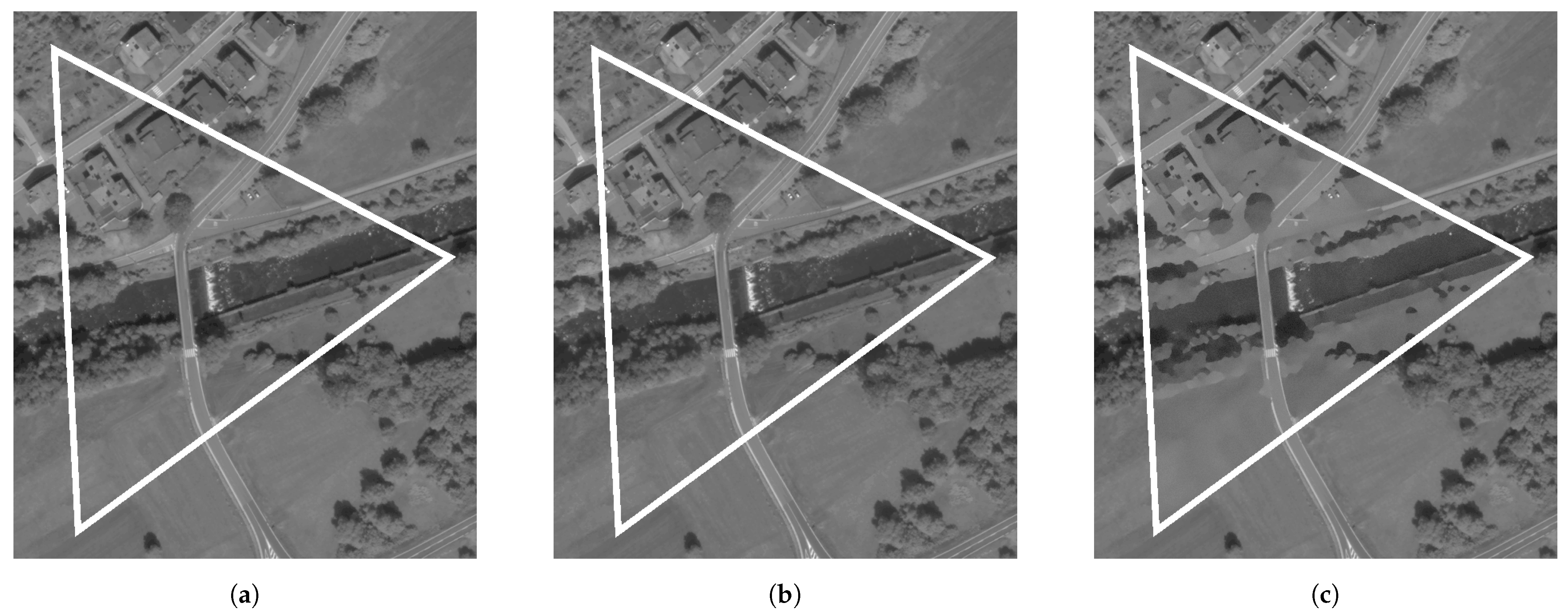
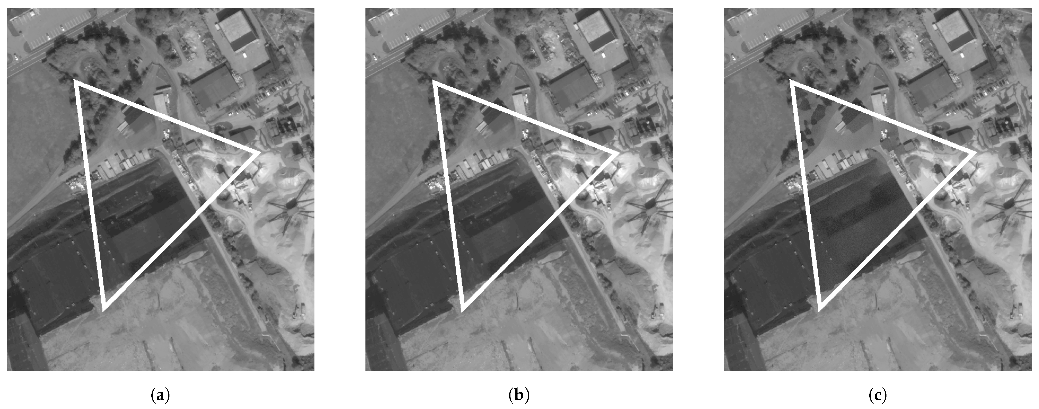
5.1.1. Self-Validation Test on a Single Worldview-3 Band

The procedure was applied to a single WorldView-3 band (Panchromatic, 11-bit radiometric resolution, 40 cm spatial resolution, 5870 × 3660 pixels). The test was conceived to demonstrate the performance in reconstructing spatially complex structures.

• Band: Panchromatic (P)—segmentation parameters $\mathit{\alpha }$ = 4000, $\mathit{\lambda }$ = 20

Figure 2 shows the base image, and the artificially degraded target image is shown in Figure 3. The results obtained by variational segmentation with HM and ED based radiometric reconstructions are shown in Figure 4 and Figure 5, respectively. In 

Table 1. Error characteristics of panchromatic self-validation tests with $(\alpha ,\lambda )=(4000,20)$; mean of intensity differences, variance of intensity differences, coefficient of determination.

	HM			ED
	${\mathit{\mu }}_{\mathit{E}}$	${\mathit{\sigma }}_{\mathit{E}}^{\mathit{2}}$	${\mathit{R}}^{\mathit{2}}$	${\mathit{\mu }}_{\mathit{E}}$	${\mathit{\sigma }}_{\mathit{E}}^{\mathit{2}}$	${\mathit{R}}^{\mathit{2}}$
P	$0.002$	$0.013$	$0.999$	$-0.423$	$256.313$	$0.932$

, error statistics of HM and ED reconstructions are reported. For each reconstruction approach, mean, variance, and coefficient of determination $R^2$ of the differences between original and reconstructed values are given. Scatter plots of the differences are shown in Figure 6a,b.

Figure 7 shows a portion of the WorldView-3 scene, and its corresponding variational approximation u on the first and second rows, respectively; in the third row, the discontinuity function s is plotted along with the base clumps.

In the left columns of Figure 8 and Figure 9, two details of the WorldView-3 scene are shown, and the results of the HM and SVM reconstructions are plotted on the center and on the right columns, respectively.

As can be seen in Figure 8 and Figure 9, the quality of the reconstruction is very high essentially because of the geometrical and radiometric information enhancement produced by the Mumford–Shah segmentation and the following detection of coherent regions used in the radiometric analysis.

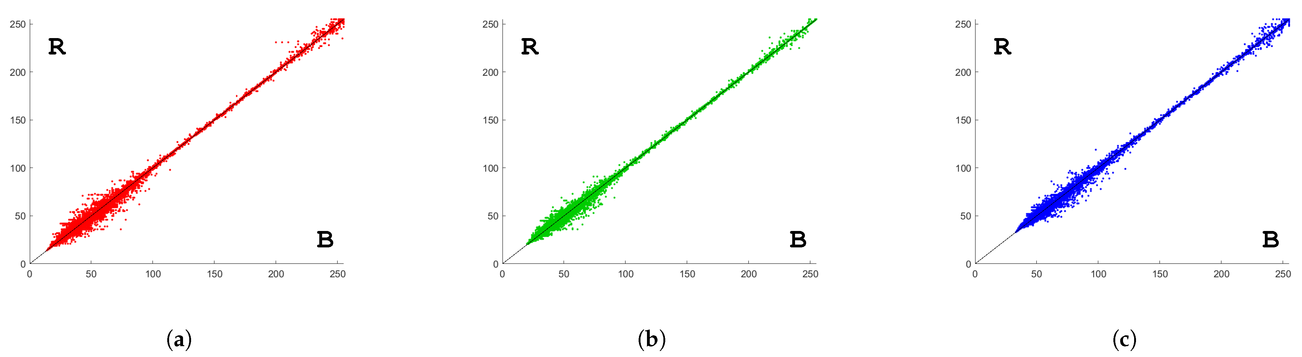
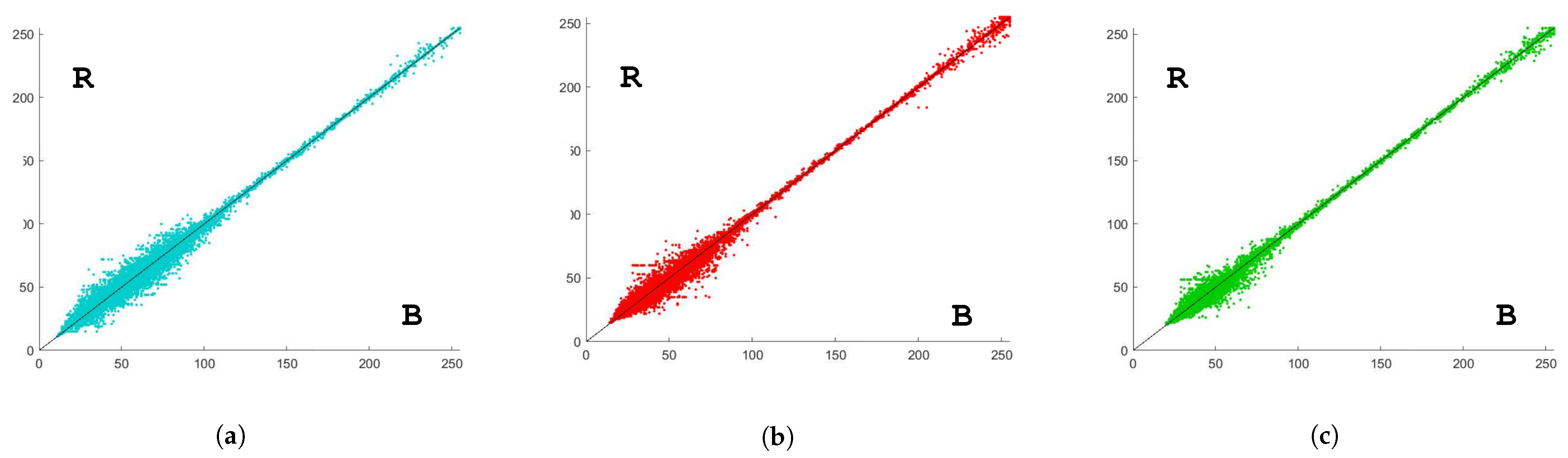
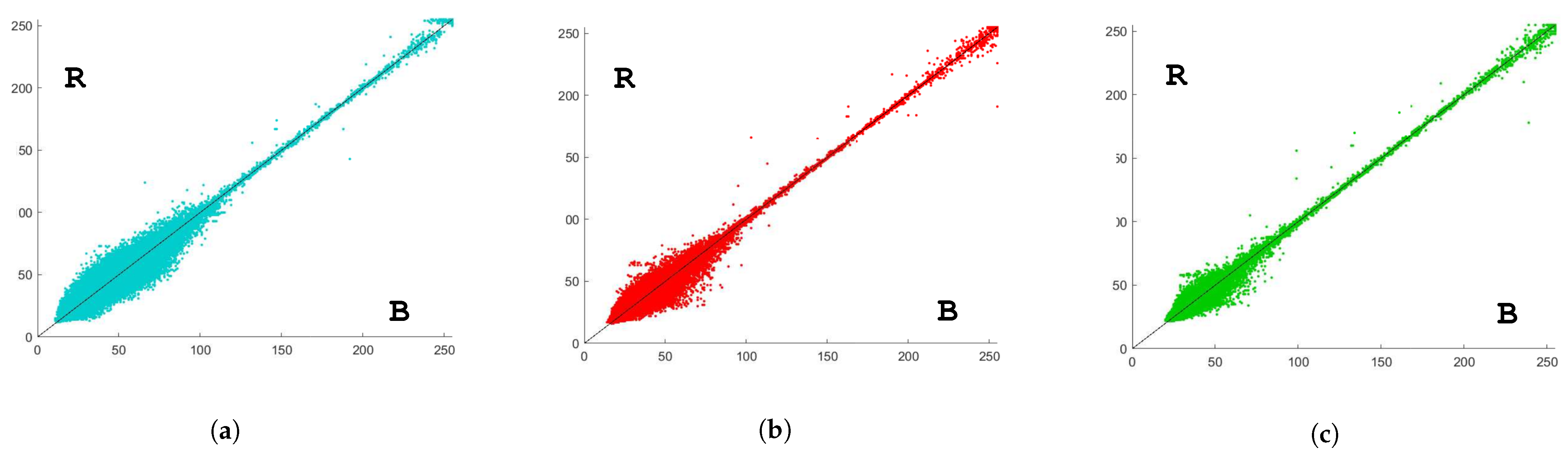
5.1.2. Self-Validation Tests on a Set of Landsat 7 Bands

The procedure was applied to the Landsat 7 LE71920282000332NSG00 scene which does not present SLC-off defects (Data acquired in mid 2000, before SLC failure). The scene that served as base imagery was artificially damaged by applying SLC-off like gaps to produce target imagery. Original and reconstructed data for a couple of three-band subsets are hereafter presented in order to evaluate the performance of the procedure. In the segmentation phase, about ten tests were performed with different values of the parameters ($\alpha$, $\lambda$). In each test reported hereafter, the same values of the parameters ($\alpha$, $\lambda$) were used for segmentation of base and target bands. The selected parameters are those which led to the best results in the tests. For comparison, each test is complemented by the statistics of results obtained using different pairs of parameter values; for these tests, the reconstructed imagery were qualitatively very similar to those reported in this section.

• Band set: Red, Green, Blue (RGB)—segmentation parameters $\mathit{\alpha }$ = 500, $\mathit{\lambda }$ = 8

Figure 10 shows base, target, HM, and ED reconstructions. In the figure, colors were artificially altered only after processing and just to facilitate the visual interpretation; the pixel brightness level in RGB space was manually modified using the GNU Image Manipulation Program (GIMP). In 

Table 2. Error characteristics of RGB self-validation tests with $(\alpha ,\lambda )=(500,8)$; mean of intensity differences, variance of intensity differences, coefficient of determination.

	HM			ED
	${\mathit{\mu }}_{\mathit{E}}$	${\mathit{\sigma }}_{\mathit{E}}^{\mathit{2}}$	${\mathit{R}}^{\mathit{2}}$	${\mathit{\mu }}_{\mathit{E}}$	${\mathit{\sigma }}_{\mathit{E}}^{\mathit{2}}$	${\mathit{R}}^{\mathit{2}}$
R	$-0.013$	$0.555$	$0.999$	$0.037$	$6.020$	$0.989$
G	$-0.009$	$0.542$	$0.999$	$-0.037$	$8.196$	$0.986$
B	$-0.008$	$0.867$	$0.999$	$-0.054$	$18.071$	$0.996$

, error statistics of HM and ED reconstructions are reported. For each reconstruction approach, mean, variance, and coefficient of determination $R^2$ of the differences between original and reconstructed values are given. Scatter plots of the differences are shown in Figure 11 and Figure 12. For comparison, error statistics of HM and ED reconstructions obtained with different values of the segmentation parameters $(\alpha ,\lambda )=(1200,8)$ and leading to worse results are reported in 

Table 3. Error characteristics of RGB self-validation tests with $(\alpha ,\lambda )=(1200,8)$, reported for comparison with Table 2; mean of intensity differences, variance of intensity differences, and coefficient of determination.

	HM			ED
	${\mathit{\mu }}_{\mathit{E}}$	${\mathit{\sigma }}_{\mathit{E}}^{\mathit{2}}$	${\mathit{R}}^{\mathit{2}}$	${\mathit{\mu }}_{\mathit{E}}$	${\mathit{\sigma }}_{\mathit{E}}^{\mathit{2}}$	${\mathit{R}}^{\mathit{2}}$
R	$-0.015$	$1.542$	$0.998$	$-0.054$	$21.942$	$0.968$
G	$-0.013$	$1.003$	$0.998$	$-0.034$	$10.039$	$0.982$
B	$-0.012$	$0.955$	$0.998$	$-0.056$	$7.330$	$0.969$

.

• Band set: Near-infrared, Red, Green (NRG)—segmentation parameters $\mathit{\alpha }$ = 500, $\mathit{\lambda }$ = 8

Figure 13 shows base, target, and HM reconstruction. In 

Table 4. Error characteristics of NRG self-validation tests with $(\alpha ,\lambda )=(500,8)$; mean of intensity differences, variance of intensity differences, and coefficient of determination.

	HM			ED
	${\mathit{\mu }}_{\mathit{E}}$	${\mathit{\sigma }}_{\mathit{E}}^{\mathit{2}}$	${\mathit{R}}^{\mathit{2}}$	${\mathit{\mu }}_{\mathit{E}}$	${\mathit{\sigma }}_{\mathit{E}}^{\mathit{2}}$	${\mathit{R}}^{\mathit{2}}$
N	$0.022$	$2.579$	$0.996$	$-0.071$	$26.062$	$0.947$
R	$-0.031$	$1.774$	$0.997$	$0.090$	$16.773$	$0.976$
G	$0.021$	$1.080$	$0.998$	$0.072$	$7.456$	$0.987$

, error statistics of HM and ED reconstructions are reported. For each reconstruction approach, mean, variance, and coefficient of determination $R^2$ of the differences between original and reconstructed values are given. Scatter plots of the differences are shown in Figure 14 and Figure 15. For comparison, error statistics of HM and ED reconstructions obtained with different values of the segmentation parameters $(\alpha ,\lambda )=(1600,12)$ and leading to worse results are reported in 

Table 5. Error characteristics of NRG self-validation tests with $(\alpha ,\lambda )=(1600,12)$, reported for comparison with Table 4; mean of intensity differences, variance of intensity differences, and coefficient of determination.

	HM			ED
	${\mu }_E$	${\mathit{\sigma }}_{\mathit{E}}^{\mathit{2}}$	${\mathit{R}}^{\mathit{2}}$	${\mathit{\mu }}_{\mathit{E}}$	${\mathit{\sigma }}_{\mathit{E}}^{\mathit{2}}$	${\mathit{R}}^{\mathit{2}}$
N	$0.010$	$3.718$	$0.995$	$-0.134$	$62.845$	$0.910$
R	$0.003$	$2.819$	$0.996$	$-0.127$	$24.728$	$0.964$
G	$0.001$	$1.790$	$0.997$	$-0.102$	$11.243$	$0.980$

.

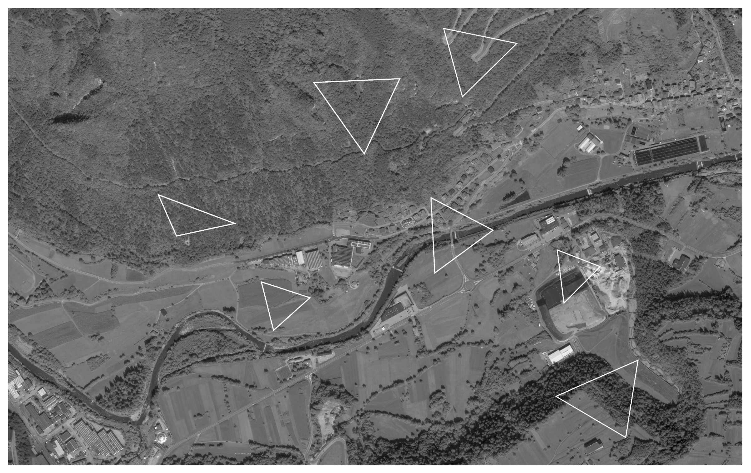
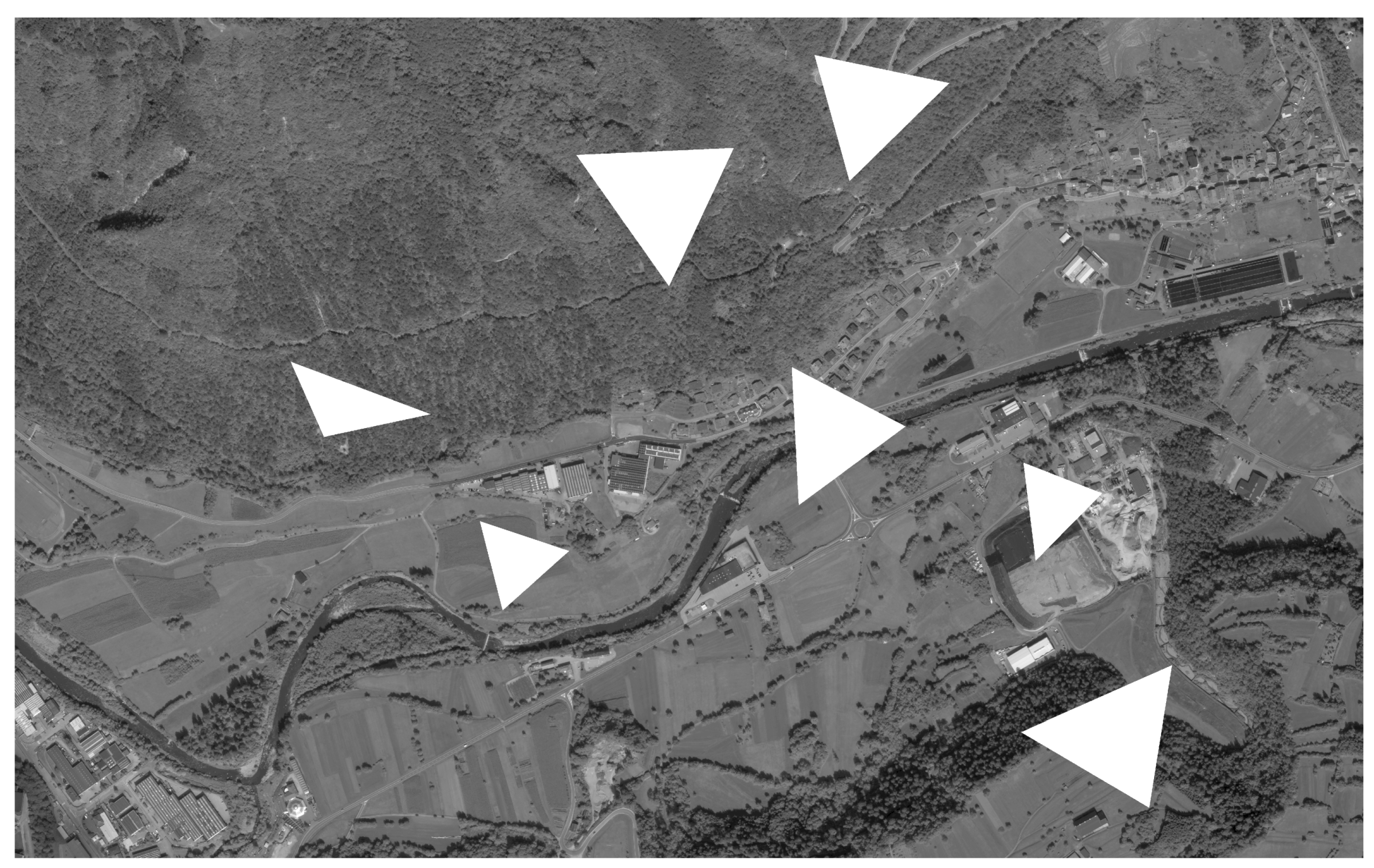
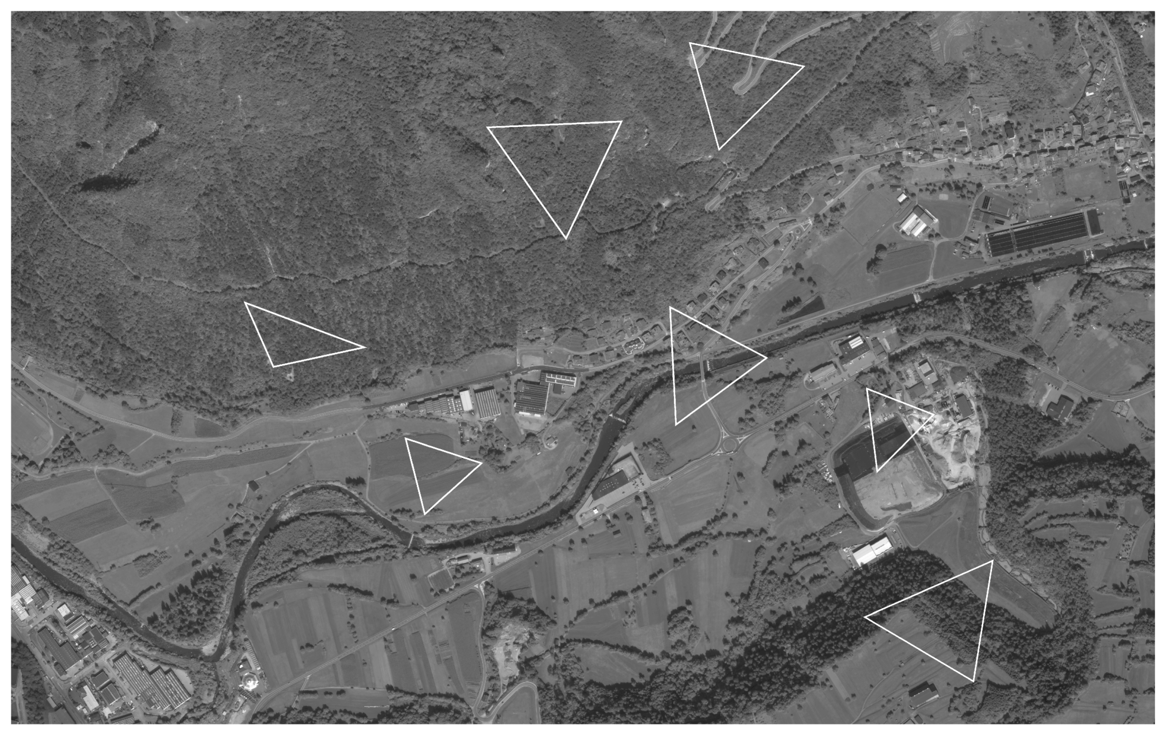
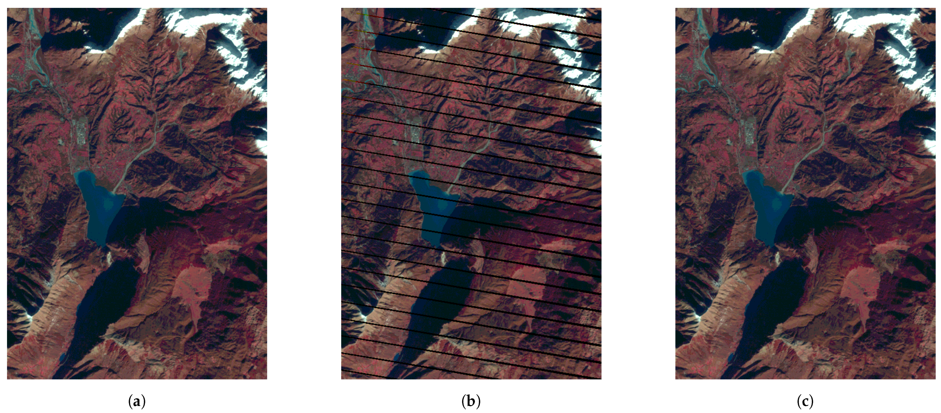
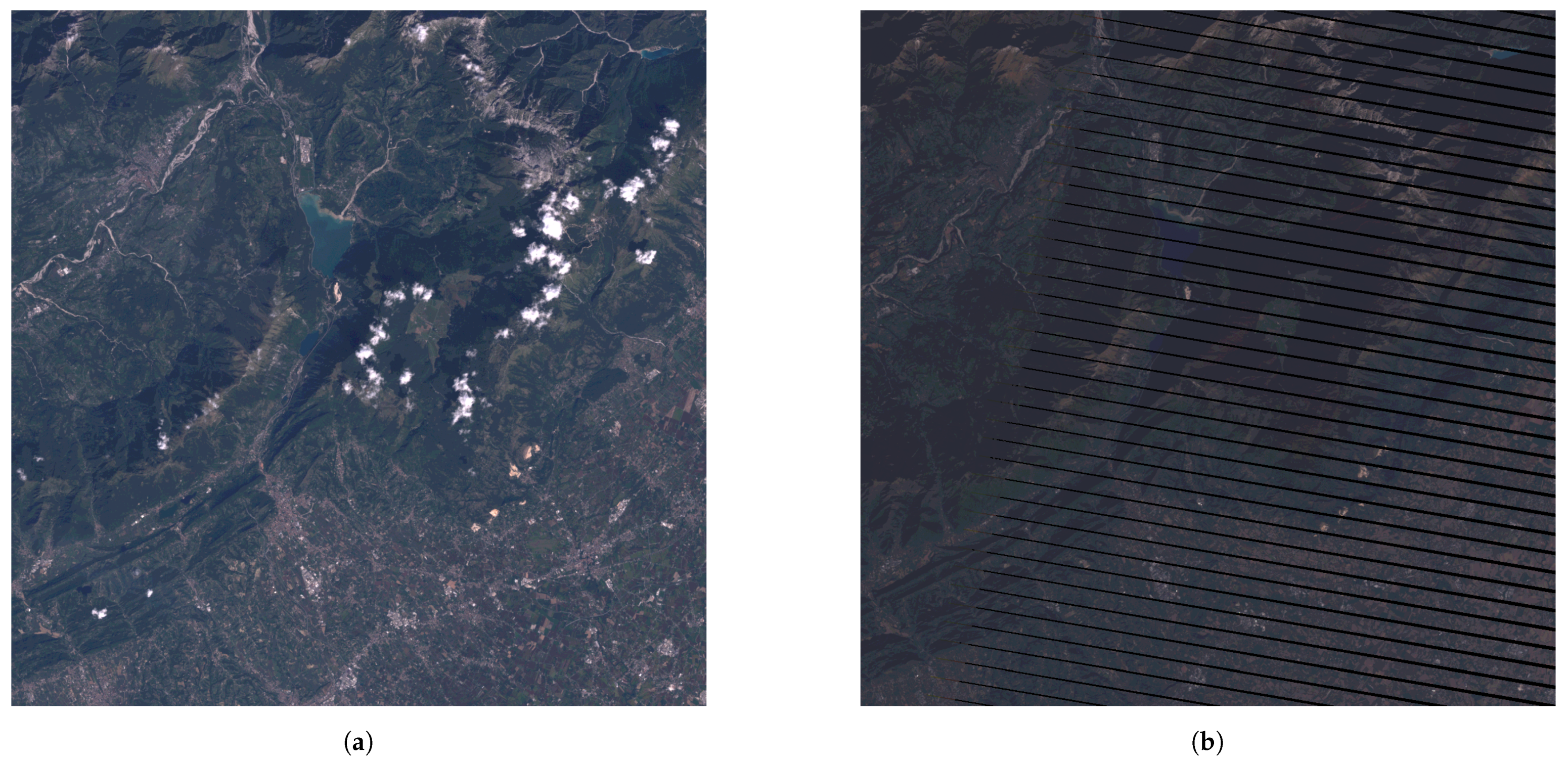
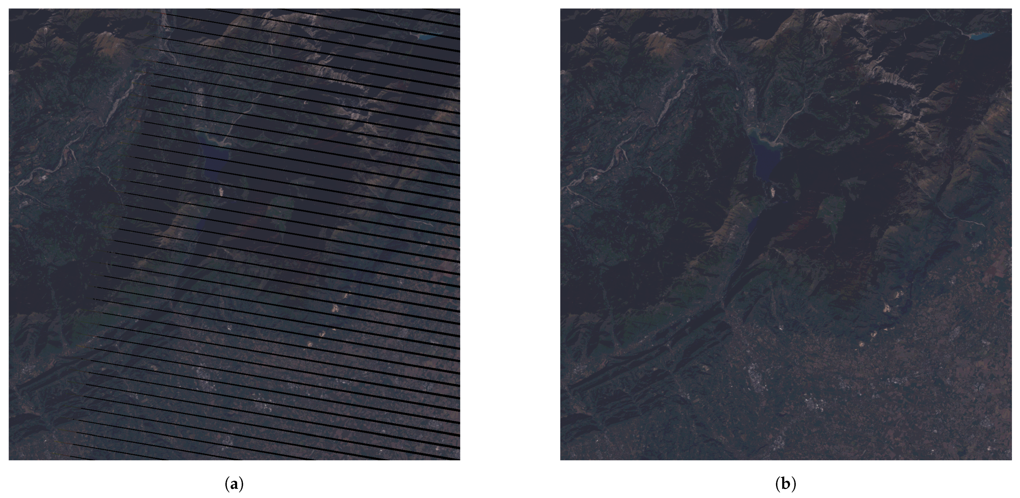
5.2. Real Case Applications

The procedure was applied to the Landsat 7 target scene LE71920282014306NSG100 affected by SLC-off disturbances and considering the disturbances-free Landsat 7 scene LE71920282002257EDC00 as base imagery, see Figure 16.

Variational segmentation was applied to base and target bands, the Mumford–Shah parameters ($\alpha$, $\lambda$) were set to $(500,8)$ for base bands and to $(100,4)$ for target bands, Step 1 in Figure 1.

Figure 17 shows the labeled connected components (clumps) of the base and target RGB three-band sets, Step 3 in Figure 1.

In Figure 18, the scheme behind the radiometric reconstruction approaches is represented: base image (B) is shown on the left in Figure 18a, target image (T) is on the right; in Figure 18b, region boundaries, built after connected components identification, are overlaid to base and target images, and one region to be reconstructed is plotted in green; in Figure 18c, coherent regions corresponding to the region to be reconstructed are plotted in light green in the base image; in Figure 18d, coherent regions corresponding to the region to be reconstructed are plotted in light blue in the target image.

Figure 19 shows the target and the HM reconstructed RGB images, a zoomed region is shown in Figure 20. In the figure, colors were artificially altered only after processing and just to facilitate the visual comparison; the pixel brightness curve in RGB space was manually modified using the GNU Image Manipulation Program (GIMP).

6. Discussion

Variational image segmentation has proven instrumental in image restoration: the smoothing action, by reducing the noise level of input data, and the discontinuity-preserving feature eases the identification of homogeneous regions and hence the forming of coherent region sets to be used in the radiometric analysis on which the reconstruction is based. Identification of coherent region sets is carried out by means of bands composition, clumping, and cross products of intensity levels of base and target images. Together, these features also allow the reconstruction of geometrically complex scenes (see Figure 5). In the variational segmentation, for a given spatial resolution, the use of high parameter values will lead to better results when processing lowly fragmented scenes, lower values are instead recommended for more complex scenes, such as mountain and urban areas. To guide the selection of suitable parameter values, it can be suggested to execute some tests on a not-damaged portion of a scene and to assess the results on the basis of a self-validation like scenario.

Two different applications have been proposed, both fulfilling their purposes with valid results as reported in Table 2 and Table 4 where small mean errors are essentially due to the rounding integer necessary to respect data type of DNs. Reconstruction is not operated by simply picking data from neighboring pixels but by relying on a procedure that links different coherent regions on a radiometric basis. Applications showed a better performance of the HM based reconstruction approach when compared to the ED one. Differences increase when just a single band is processed and when high spatial resolution data are considered. This is essentially due to the capability of the HM approach to reproduce inter-region radiometric patterns, to the choice of Gaussian distribution sampling, and to the lower sensitivity of HM transformation to non Gaussian-like ECDFs. In this framework, the use of power transform could be considered [23,24]. Power transform is a family of functions that are applied to create a monotonic transformation of data using power functions. This is a useful data transformation technique that stabilizes variance and produces more normally distributed samples.

From a practical point of view, the proposed procedure could be incorporated in a more articulated satellite image processing framework involving cloud, cloud shadow, and snow detection algorithms [25,26]. Preliminary results also showed a strong positive impact of variational segmentation as a preprocess step in pansharpening and super resolution mapping applications.

From the analytical point of view, a possible development regards the adoption of an advanced and more complex variational model for image segmentation. In the Mumford–Shah model, the presence of the gradient norm (the smoothing term) permits only near-constant piece-wise solutions. In satellite images, regions with radiometric steep gradients are common and the Mumford–Shah approximation may present staircase-like artifacts in such regions. Owen [27] proposed a second order variational model to overcome limitations of the Mumford–Shah model. Solutions produced by the Blake–Zisserman model are basically nearly-linear piece-wise approximations of the data [22,28,29,30,31,32].

References

1. Aubert, G.; Kornprobst, P. Mathematical Problems in Image Processing; Springer: New York, NY, USA, 2006. [Google Scholar] [CrossRef] [Green Version]
2. Zhang, Q.; Yuan, Q.; Zeng, C.; Li, X.; Wei, Y. Missing Data Reconstruction in Remote Sensing Image with a Unified Spatial–Temporal–Spectral Deep Convolutional Neural Network. IEEE Trans. Geosci. Remote Sens. 2018, 56, 4274–4288. [Google Scholar] [CrossRef] [Green Version]
3. Zhu, J.; Li, K.; Hao, B. Restoration of remote sensing images based on nonconvex constrained high-order total variation regularization. J. Appl. Remote Sens. 2019, 13, 1–17. [Google Scholar] [CrossRef]
4. Shen, H.; Li, X.; Cheng, Q.; Zeng, C.; Yang, G.; Li, H.; Zhang, L. Missing Information Reconstruction of Remote Sensing Data: A Technical Review. IEEE Geosci. Remote Sens. Mag. 2015, 3, 61–85. [Google Scholar] [CrossRef]
5. Ali, L.; Kasetkasem, T.; Khan, W.; Chanwimaluang, T.; Nakahara, H. Performance evaluation of different inpainting algorithms for remotely sensed images. In Proceedings of the 2017 Third Asian Conference on Defence Technology (ACDT), Phuket, Thailand, 18–20 January 2017; pp. 43–48. [Google Scholar] [CrossRef]
6. Dong, J.; Yin, R.; Sun, X.; Li, Q.; Yang, Y.; Qin, X. Inpainting of Remote Sensing SST Images With Deep Convolutional Generative Adversarial Network. IEEE Geosci. Remote Sens. Lett. 2019, 16, 173–177. [Google Scholar] [CrossRef]
7. Chen, J.; Zhu, X.; Vogelmann, J.E.; Gao, F.; Jin, S. A simple and effective method for filling gaps in Landsat ETM+ SLC-off images. Remote Sens. Environ. 2011, 115, 1053–1064. [Google Scholar] [CrossRef]
8. Brooks, E.; Wynne, R.; Thomas, V. Using Window Regression to Gap-Fill Landsat ETM+ Post SLC-Off Data. Remote Sens. 2018, 10, 1502. [Google Scholar] [CrossRef] [Green Version]
9. Qureshi, M.A.; Deriche, M.; Beghdadi, A.; Amin, A. A critical survey of state-of-the-art image inpainting quality assessment metrics. J. Vis. Commun. Image Represent. 2017, 49, 177–191. [Google Scholar] [CrossRef]
10. Asare, Y.M.; Forkuo, E.K.; Forkuor, G.; Thiel, M. Evaluation of gap-filling methods for Landsat 7 ETM+ SLC-off image for LULC classification in a heterogeneous landscape of West Africa. Int. J. Remote Sens. 2020, 41, 2544–2564. [Google Scholar] [CrossRef]
11. Mumford, D.; Shah, J. Optimal Approximations by Piecewise Smooth Functions and Associated Variational Problems. Commun. Pure Appl. Math. 1989, 42, 577–685. [Google Scholar] [CrossRef] [Green Version]
12. Zambelli, P.; Gebbert, S.; Ciolli, M. Pygrass: An Object Oriented Python Application Programming Interface (API) for Geographic Resources Analysis Support System (GRASS) Geographic Information System (GIS). ISPRS Int. J. Geo-Inf. 2013, 2, 201–219. [Google Scholar] [CrossRef] [Green Version]
13. Scaramuzza, P.; Micijevic, E.; Gyanesh, C. SLC Gap-Filled Products—Phase One Methodology. Available online: https://www.usgs.gov/media/files/landsat-7-slc-gap-filled-products-phase-one-methodology (accessed on 1 December 2020).
14. USGS. SLC Gap-Filled Products—Phase Two Methodology. Available online: https://www.usgs.gov/media/files/landsat-7-slc-gap-filled-products-phase-two-methodology (accessed on 1 December 2020).
15. Aghamohamadnia, M.; Abedini, A. A morphology-stitching method to improve Landsat SLC-off images with stripes. Geod. Geodyn. 2014, 5, 27–33. [Google Scholar] [CrossRef] [Green Version]
16. Zhang, C.; Li, W.; Travis, D. Gaps-fill of SLC-off Landsat ETM+ satellite image using a geostatistical approach. Int. J. Remote Sens. 2007, 28, 5103–5122. [Google Scholar] [CrossRef]
17. Gaohong, Y.; McCabe, M.F.; Mariethoz, G. Gap-Filling of Landsat 7 Imagery Using the Direct Sampling Method. Remote Sens. 2016, 9, 12. [Google Scholar]
18. De Giorgi, E. Free discontinuity problems in calculus of variations. In Frontiers in Pure and Applied Mathemathics, a Collection of Papers Dedicated to J.L. Lions on the Occasion of His 60th Birthday; Dautray, R., Ed.; North Holland: Amsterdam, The Netherlands, 1991; pp. 55–62. [Google Scholar]
19. De Giorgi, E.; Carriero, M.; Leaci, A. Existence theorem for a minimum problem with free discontinuity set. Arch. Ration. Mech. Anal. 1989, 108, 195–218. [Google Scholar] [CrossRef]
20. Ambrosio, L.; Fusco, N.; Pallara, D. Functions of Bounded Variation and Free Discontinuity Problems; Oxford University Press: Oxford, UK, 2000. [Google Scholar]
21. Modica, L.; Mortola, S. Un esempio di Gamma-convergenza. Boll. dell’Unione Matatematica Ital. 1977, B-14, 285–299. [Google Scholar]
22. Vitti, A. The Mumford–Shah variational model for image segmentation: An overview of the theory, implementation and use. ISPRS J. Photogramm. Remote Sens. 2012, 69, 50–64. [Google Scholar] [CrossRef]
23. Yeo, I.K.; Johnson, R.A. A New Family of Power Transformations to Improve Normality or Symmetry. Biometrika 2000, 87, 954–959. [Google Scholar] [CrossRef]
24. Box, G.E.P.; Cox, D.R. An Analysis of Transformations. J. R. Stat. Soc. Ser. B (Methodol.) 1964, 26, 211–243. [Google Scholar] [CrossRef]
25. Baetens, L.; Desjardins, C.; Hagolle, O. Validation of Copernicus Sentinel-2 Cloud Masks Obtained from MAJA, Sen2Cor, and FMask Processors Using Reference Cloud Masks Generated with a Supervised Active Learning Procedure. Remote Sens. 2019, 11, 433. [Google Scholar] [CrossRef] [Green Version]
26. Zhu, Z.; Woodcock, C.E. Automated cloud, cloud shadow, and snow detection in multitemporal Landsat data: An algorithm designed specifically for monitoring land cover change. Remote Sens. Environ. 2014, 152, 217–234. [Google Scholar] [CrossRef]
27. Owen, T. Visual Reconstruction by Andrew Blake and Andrew Zisserman, The MIT Press, Massachusetts, USA, 1987, 1987 (£22.50). Robotica 1988, 6, 166. [Google Scholar] [CrossRef]
28. Carriero, M.; Leaci, A.; Tomarelli, F. Free gradient discontinuity and image inpainting. J. Math. Sci. 2012, 181, 805–819. [Google Scholar] [CrossRef]
29. Borghi, A.; Cannizzaro, L.; Vitti, A. Advanced techniques for discontinuity detection in GNSS coordinate time-series. An Italian case study. In International Association of Geodesy Symposia; Springer: Berlin, Germany, 2012; Volume 136, pp. 627–634. [Google Scholar] [CrossRef]
30. Vitti, A. Sigseg: A tool for the detection of position and velocity discontinuities in geodetic time-series. GPS Solut. 2012, 16, 405–410. [Google Scholar] [CrossRef]
31. Zanetti, M.; Vitti, A. The Blake-Zisserman model for digital surface models segmentation. ISPRS Ann. Photogramm. Remote Sens. Spat. Inf. Sci. 2013, II-5/W2, 355–360. [Google Scholar] [CrossRef] [Green Version]
32. Benciolini, B.; Ruggiero, V.; Vitti, A.; Zanetti, M. Roof planes detection via a second-order variational model. ISPRS J. Photogramm. Remote Sens. 2018, 138, 101–120. [Google Scholar] [CrossRef]
Figure 1. Flowchart of the proposed procedure for image reconstruction.
Ijgi 10 00017 g001
Figure 2. Base image.
Ijgi 10 00017 g002
Figure 3. Target image.
Ijgi 10 00017 g003
Figure 4. HM reconstruction.
Ijgi 10 00017 g004
Figure 5. ED reconstruction.
Ijgi 10 00017 g005
Figure 6. Panchromatic self-validation test—radiometric reconstructions; B = Base intensity values, R = Reconstructed intensity values. (a) Scatter plot of Panchromatic values—HM based reconstruction; (b) scatter plot of Panchromatic values—ED based reconstruction.
Ijgi 10 00017 g006
Figure 7. WorldView-3 image and intermediate maps. (a) panchromatic band; (b) variational approximation u of WorldView-3 Panchromatic band Figure 7a; (c) discontinuity function s with clumps of the variational approximation of the base image Figure 7a.
Ijgi 10 00017 g007aIjgi 10 00017 g007b
Figure 8. Panchromatic band and radiometric reconstructions—Detail 1. (a) WorldView-3 Panchromatic band; (b) HM reconstruction; (c) ED reconstruction.
Ijgi 10 00017 g008
Figure 9. Panchromatic band and radiometric reconstructions—Detail 2. (a) WorldView-3 Panchromatic band; (b) HM reconstruction; (c) ED reconstruction.
Ijgi 10 00017 g009
Figure 10. Base, target, HM, and ED reconstructions of the RGB band set of Landsat 7 LE71920282000332NSG00 scene. (a) base image; (b) target image; (c) HM reconstruction; (d) ED reconstruction.
Ijgi 10 00017 g010
Figure 11. RGB self-validation test—HM based reconstruction; B = Base intensity values, R = Reconstructed intensity values. (a) scatter plot of red values; (b) scatter plot of green values; (c) scatter plot of blue values.
Ijgi 10 00017 g011
Figure 12. RGB self-validation test—ED based reconstruction; B = Base intensity values, R = Reconstructed intensity values. (a) scatter plot of red values; (b) scatter plot of green values; (c) scatter plot of blue values.
Ijgi 10 00017 g012
Figure 13. Base, target, HM reconstruction of the NRG band set of Landsat 7 LE71920282000332NSG00 scene. (a) base image; (b) target image; (c) HM reconstruction.
Ijgi 10 00017 g013
Figure 14. NRG self-validation test—HM based reconstruction; B = Base intensity values, R = Reconstructed intensity values. (a) scatter plot of Near-infrared values; (b) scatter plot of Red values; (c) scatter plot of Green values.
Ijgi 10 00017 g014
Figure 15. NRG self-validation test—ED based reconstruction; B = Base intensity values, R = Reconstructed intensity values. (a) scatter plot of near-infrared values; (b) scatter plot of red values; (c) scatter plot of green values.
Ijgi 10 00017 g015
Figure 16. Base and target images from LE71920282002257EDC00 and LE71920282014306NSG100 Landsat 7 scenes. (a) base image; (b) target image.
Ijgi 10 00017 g016
Figure 17. Clump maps for base and target images of Figure 16. (a) base clumps; (b) target clumps.
Ijgi 10 00017 g017
Figure 18. Scheme for the construction of radiometric data set for reconstruction. (a) base and target images; (b) base and target images with red region boundaries and one region in green; (c) base and target images with red region boundaries and one region in green and with base coherent regions in light green; (d) base and target images with red region boundaries and one region in green, base coherent regions in light green and with target coherent regions in light blue.
Ijgi 10 00017 g018
Figure 19. Target and HM reconstruction, see Figure 16. (a) target image; (b) HM reconstruction.
Ijgi 10 00017 g019
Figure 20. Target and HM reconstruction (portion of), see Figure 16. (a) target image; (b) HM reconstruction.
Ijgi 10 00017 g020