Thunder Dynamics: A C++ Tool for Adaptive Control of Serial Manipulators

Abstract

Robust control techniques are crucial for deploying robotic solutions in real applications and handling model uncertainties in robotic manipulators. The inertial parameters are fundamental to implementing control algorithms. While theoretical approaches to compute the system dynamics and the regressor matrix are well-established, they are computationally expensive and a practical implementation framework is still lacking. To address this challenge, we developed a new and efficient method to compute the Coriolis matrix based on Christoffel’s symbols. The result forms the basis of Thunder Dynamics, an open-source software package able to create standalone libraries that compute the system kinematics and dynamics for real-time adaptive control implementation. Thunder Dynamics enables users to create and compile user-defined functions on a robot, which can then be used in C++ or Python 3. To test the proposed framework, we implemented a Cartesian adaptive backstepping controller with axis-angle orientation using our tool. We tested the controller on a seven-degrees-of-freedom manipulator in both simulation and real-world scenarios, varying the levels of uncertainties in the inertial parameters. The results demonstrated that Thunder Dynamics is capable of meeting computational constraints given by the control loop frequency of real systems, permitting, for example, the implementation of advanced controls on commercial manipulators.

1. Introduction

At present, the usage of robotic manipulators is exponentially increasing in a large number of fields, such as manufacturing, logistics, and healthcare [1,2,3]. This trend is motivated by the ability of this type of system to perform motions with an extremely high level of precision and to handle heavy loads.

Underlying the level of performance achieved, there is a strong theoretical background provided by the study of the dynamics of rigid bodies [4]. Over time, researchers have developed a large set of algorithms to compute different entities related to rigid body systems, such as forward and backward dynamics, in an efficient way [5]. From these results, in the last decade, different software packages that allow for the easy implementation of all these algorithms have been released [6,7]. However, this type of approach is feasible only if we have perfect knowledge of the mechanical properties of each link in the manipulator. In this case, if the robot picks an object to perform the desired task, the inertia of the grasped object will change the dynamic behavior of the kinematic chain.

Different strategies have been proposed in the literature to compensate for the effect of uncertainties in the model. There are two principal types of solution: model identification and adaptive control. The first type tackles the problem offline by setting up an estimation procedure to identify the unknown parameters [8]. The latter targets the problem online from a control perspective by adapting the control action to compensate for parameter uncertainties. These types of solutions are usually called adaptive controllers [9,10]. The most famous algorithm in this family is the one proposed in [11], where the control law is composed of feedback and feedforward parts, while parameters are modified online to ensure stability. In recent decades, there have been a large number of studies in this research field, covering several aspects of this problem [12,13,14,15,16,17,18]. Even if this approach is effective in compensating for model errors, it requires the factorization of the robot dynamic equation to be explicitly expressed in a linear form with respect to the inertial parameters [19]. Usually, this factorization uses the classical inertial representation of rigid bodies. However, the computation of the regressor matrix, which can be easily achieved through the inspection of manipulators with a couple of Degrees of Freedom (DoFs), is a daunting task for many-DoFs systems.

Works that address this problem include [20,21], where the authors proposed algorithms to build the regressor and the dynamical matrices related to the inertial parameters. In [21], the authors also proposed a library, developed in Wolfram Mathematica©, that integrates the algorithm for generating this regressor through Denavit–Hartenberg (DH) representation [22], considering serial kinematic structures. However, the existing solutions cannot be integrated in a straightforward manner into a classical software control infrastructure, which is usually developed in a ROS framework using languages like C++ or Python. Existing libraries often focus on the fast implementation of rigid-body dynamics algorithms [7], or are tailored to floating base [23] and multi-contact systems [24]. The growing research interest in machine learning has also moved the community toward differentiable dynamic frameworks [25]. Recently, the authors in [26] developed a high-level Python toolbox based on Pinocchio library. However, the proposed tool is designed for the identification and calibration of robot inertial parameters and, to the best of our knowledge, it does not provide information that can be used for the online implementation of adaptive controllers. Moreover, while a few object-oriented attempts have improved modularity [27,28], most solutions remain hard for the average user to upgrade or adapt.

In this work, we present Thunder Dynamics, a software package based on C++ and CasADi [29], for the implementation of the adaptive control on serial manipulators. In contrast with other solutions presented in the literature, our framework is built from the ground-up to be easily expandable and to generate fine-tuned C++ (or Python) libraries for any serial manipulator application. To develop this tool, we started with the results obtained in [21], and we formulated a procedure that does not require high-order tensor algebra to compute the dynamic regressor and can be easily implemented with standard software languages within a short computational time. To test the effectiveness of our method, we provided a task-space adaptive backstepping controller and we used our tool to implement the control algorithm for the 7 DoFs manipulator Franka Emika Panda. This controller is applied both in simulations and to the real system in different scenarios. The aim is to test the ability of the proposed tools to provide all the needed quantities for computing the control action without violating the control loop frequency constraint of the controlled system. These tests show that the C++ library generated with Thunder Dynamics is fast enough to implement an adaptive controller in real time.

The paper is organized as follows: in Section 2, we briefly recall the theoretical background needed for the manuscript. In Section 3, we describe the software package and structure of Thunder Dynamics from a user perspective to provide a simple understanding. Then, the particular focus is on the new formulation used to compute the Coriolis Matrix and how to exploit this to derive an explicit Slotine-Li regressor. In Section 4, we derive the Adaptive Backstepping Control with the axis-angle rotation representation. Then, in Section 5, we validate the effectiveness of the generated library on the proposed control framework. We test this on a seven-DoFs Franka Emika Panda robot. The experiments are performed both in simulations and in the real world. Finally, Section 6 concludes the paper with our considerations.

2. Theorethical Background

2.1. Serial Manipulators

In this section, we recall the basic equations related to serial kinematic chains needed for this work. Let us define, for a serial manipulator with n joints, $q\left(t\right),\dot{q}\left(t\right),\ddot{q}\left(t\right)\in {\mathbb{R}}^n$ as the joint position, velocity, and acceleration. $\zeta \in SE\left(3\right)$ is the end-effector pose with respect to the base frame of the serial kinematic chain. $\Theta \left(q\right):q\to \zeta$ is the direct kinematics that maps joint configuration in the end-effector pose and is defined as

$$\Theta \left(q\right)=\prod _{i=1}^n{{}^{i-1}T}_i\left(q_i\right),$$

(1)

where ${{}^{i-1}T}_i$ is the transformation between the reference frame of the $i-1$ and the link i. In this work, we use the following DH parametrization to compute the transformation between two consecutive links:

$${{}^{i-1}T}_i={\mathrm{Tr}}_x\left(a_i\right){\mathrm{Rot}}_x\left({\alpha }_i\right){\mathrm{Tr}}_z\left(d_i\right){\mathrm{Rot}}_z\left({\theta }_i\right),$$

(2)

where ${\mathrm{Tr}}_j(·)$ and ${\mathrm{Rot}}_j(·)$ are elementary translation and rotation on axis j, and $a_i,{\alpha }_i,d_i$ and ${\theta }_i$ are the DH parameters. In the case of the use of URDF description, the parameters are established according to the standard convention.

Let $\xi \in {\mathbb{R}}^6$ be the end-effector twist, and $J\left(q\right)\in {\mathbb{R}}^{6\times n}$ be the geometric Jacobian matrix that maps joint velocity into the Cartesian twist, i.e.,

$$\xi \left(q\right)=J\left(q\right)\dot{q}.$$

(3)

The classical representation of the dynamic of the manipulator is

$$\tau =B\left(q\right)\ddot{q}+C(q,\dot{q})\dot{q}+G\left(q\right),$$

(4)

where $\tau \in {\mathbb{R}}^n$ is the torque applied to the joint, and $B\left(q\right)$, $C(q,\dot{q})\in {\mathbb{R}}^{n\times n}$, and $G\left(q\right)\in {\mathbb{R}}^n$, are the inertia and Coriolis matrices, and the gravitational force vector of the serial manipulator, respectively. This formulation can be rewritten in a linear form with respect to the inertial parameters of the links of the manipulator as

$$\tau =Y(q,\dot{q},\ddot{q})\pi ,$$

(5)

where $\pi \in {\mathbb{R}}^p$ is the vector containing the inertial parameters and $Y(q,\dot{q},\ddot{q})\in {\mathbb{R}}^{n\times p}$ is the standard dynamic regressor.

From an adaptive control point of view, in [11], another version of the dynamic regressor (which, from now on, will be called Slotine-Li Regressor) has been proposed:

$$Y_r(q,\dot{q},{\dot{q}}_r,{\ddot{q}}_r)\pi =B\left(q\right){\ddot{q}}_r+C(q,\dot{q}){\dot{q}}_r+G\left(q\right),$$

(6)

where $Y_r(q,\dot{q},{\dot{q}}_r,{\ddot{q}}_r)\in {\mathbb{R}}^{n\times p}$ is the Slotine-Li regressor, and $q_r,{\dot{q}}_r$ and ${\ddot{q}}_r$ are the reference joint position, velocity, and acceleration, respectively. The peculiarity of this formulation is that it does not need the real acceleration of joints, which are difficult to measure, or have a high degree of noise if obtained from a derivative filter. For more details on the employment of this formulation of the regressor in a control framework, see Section 4.

2.2. Mathematical Notation

In this section, we report the mathematical notation used in this work. For a simple understanding,

Table 1. Notation.

${\mathit{a}}_{\mathit{i}\mathit{j}}=\mathit{A}(\mathit{i},\mathit{j})$	element in i-th row and j-th column of matrix A.
$v_i=v\left(i\right)$	element in i-th position of vector v.
$A^{r_i}$	i-th row of matrix A.
$A^{c_j}$	j-th column of matrix A.
$A_v\triangleq {\displaystyle \frac{\partial A}{\partial v}}$	derivative of matrix A with respect to v.
${}^{p,q}\left[A\right]$	reorganize the elements of the matrix/vector in p rows and in q columns.

summarizes the notation used.

In most programming languages, such as C++, matrices are typically represented as arrays of arrays. Alternatively, they can be seen as a sequence of pointers, each pointing to the memory addresses where the matrix elements are stored. Certain matrix operations can be more straightforward when the matrix is treated as a one-dimensional vector, which is achieved by reshaping the original matrix structure.

Let us consider a matrix $A\in {\mathbb{R}}^{n\times m}$ and a vector $v\in {\mathbb{R}}^p$

$$A=\left[\begin{array}{cccc}{a}_{11}& a_{12}& \dots & a_{1m}\\ a_{21}& a_{22}& \dots & a_{2m}\\ ⋮& ⋮& \ddots & ⋮\\ a_{n1}& a_{n2}& \dots & a_{nm}\end{array}\right],v=\left[\begin{array}{c}{v}_1\\ v_2\\ ⋮\\ v_p\end{array}\right],$$

we reshape A as

$${}^{1,n·m}\left[A\right]=\left[{\alpha }_1,{\alpha }_2,\dots ,{\alpha }_k,\dots {\alpha }_{n·m}\right],$$

where the conversion mapping follows the pattern

$$\begin{array}{c}\hfill A(i,j)={\alpha }_{i+(j-1)n},{\alpha }_k=A(k-(⌈k/n⌉-1)n,⌈k/n⌉),\end{array}$$

where $⌈·⌉$ is the ceiling function.

The derivative of matrix A with respect to v in computer algebra is usually defined as a matrix $A_v\in {\mathbb{R}}^{(n·m)\times p}$, i.e.,

$$A_v\triangleq {\displaystyle \frac{\partial A}{\partial v}}=\left[\begin{array}{ccc}{\displaystyle \frac{\partial a_{11}}{\partial v_1}}& \dots & {\displaystyle \frac{\partial a_{11}}{\partial v_p}}\\ ⋮& \ddots & ⋮\\ {\displaystyle \frac{\partial a_{ij}}{\partial v_1}}& \dots & {\displaystyle \frac{\partial a_{ij}}{\partial v_p}}\\ ⋮& \ddots & ⋮\\ {\displaystyle \frac{\partial a_{nm}}{\partial v_1}}& \dots & {\displaystyle \frac{\partial a_{nm}}{\partial v_p}}\end{array}\right]=\left[\begin{array}{ccc}{\displaystyle \frac{\partial {\alpha }_1}{\partial v_1}}& \dots & {\displaystyle \frac{\partial {\alpha }_1}{\partial v_p}}\\ ⋮& \ddots & ⋮\\ {\displaystyle \frac{\partial {\alpha }_k}{\partial v_1}}& \dots & {\displaystyle \frac{\partial {\alpha }_k}{\partial v_p}}\\ ⋮& \ddots & ⋮\\ {\displaystyle \frac{\partial {\alpha }_{n·m}}{\partial v_1}}& \dots & {\displaystyle \frac{\partial {\alpha }_{n·m}}{\partial v_p}}\end{array}\right].$$

Indeed, the generalized transpose operator ${(·)}^{{\top }_{t_1...t_j...t_k}}$, defined for tensors of arbitrary order, is employed. Given a tensor of k-th order ${\left(A\right)}_{i_1...i_j...i_k}=a_{i_1...i_j...i_k}$, the operator allows for the tensor indexes’ reordering to be specified, such that ${\left(A^{{\top }_{t_1...t_j...t_k}}\right)}_{i_1...i_j...i_k}=a_{i_{t_1}...i_{t_j}...i_{t_k}}$.

3. Software Package Description

In this section, we briefly describe Thunder Dynamics in Section 3.1; then, we describe our new formulation of the Coriolis matrix in Section 3.2 and how we can exploit this to derive an explicit Slotine-Li regressor in Section 3.3. The library includes all the classical terms for a serial manipulator: forward kinematics, Jacobians, dynamical matrices, and the dynamic regressor. Moreover, a framework for elastic joint structure is already present and based on the one exploited in [30]. It is important to note that adding features to the generated C++ library is a straightforward process, as outlined in Section 3.1.2.

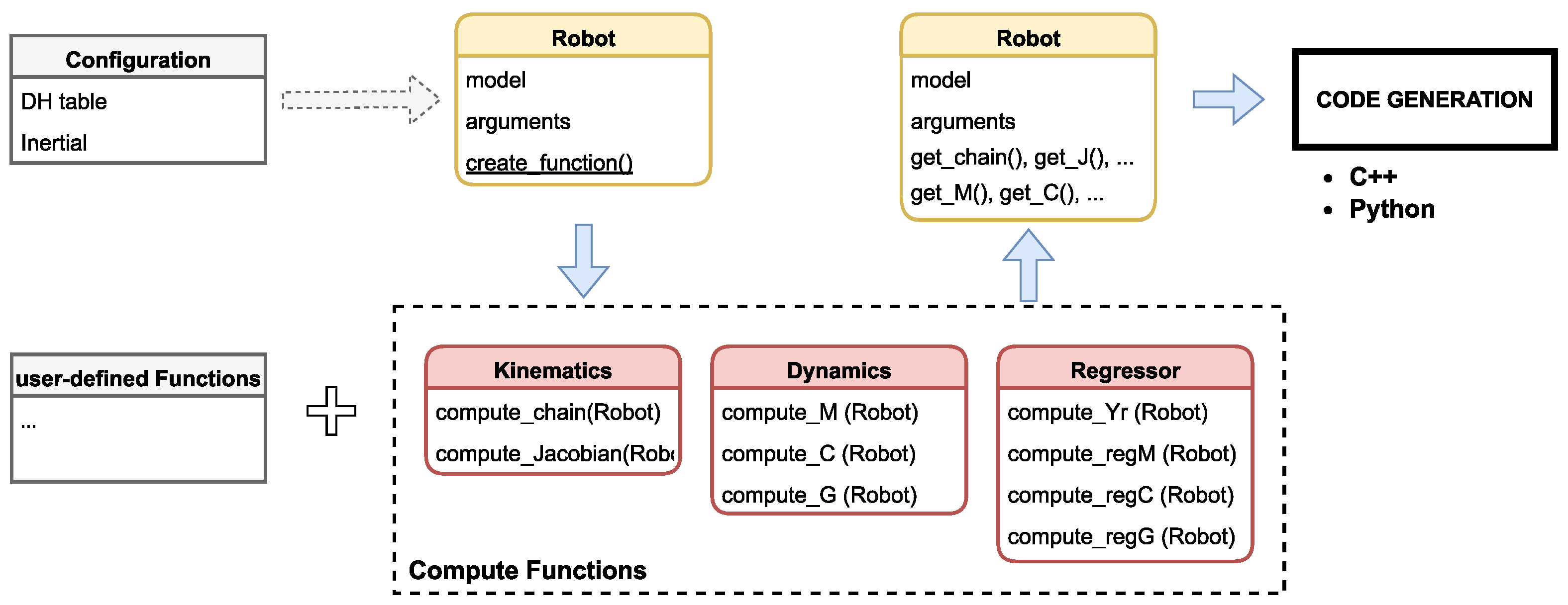
The software package is open-source and freely available (https://github.com/CentroEPiaggio/thunder_dynamics, accessed on 10 September 2025). A simplified UML diagram of the framework is depicted in Figure 1. The repository exhibits a continuous commitment to evolution, with ongoing updates that introduce additional functionalities. For a detailed explanation regarding the usage of this library, we refer the interested reader directly to the repository.

3.1. Framework User Interface

The proposed library supports two possible use cases. The first one, hereafter named High Level use case, allows the user to build a C++ system model that can be directly incorporated into the control loop. This implementation is the easiest and the fastest to use, thanks to the efficiency of the compiled C++ code. The second use case, hereafter named Low Level use case, is intended for experienced users who wish to modify the internal model, written in CasADi, to extend the library’s functionalities or to solve user-defined problems.

Both approaches require a configuration file that defines the general structure of the robot and the hyperparameters used to build the model. Specifically, this file must contain the following:

• The DH kinematic parametrization or a path to the URDF file.
• The inertial properties of the links (mass, center of mass position in the link frame, and inertia tensor expressed in the link frame).

All parameters describing the robot can be expressed either symbolically or numerically. This enables the construction of the robot model while allowing the user to choose which parameters should be treated as inputs in the high-level use case. Furthermore, the CasADi base allows for the implementation of optimization tools for optimal planning and control in a straightforward manner. Finally, the entire framework is developed inside a Docker Image to improve usability [31]. The framework is shipped with comprehensive documentation that covers installation, library generation with the command-line interface, its usage in both C++ and Python, and step-by-step guides for extending the model by enabling symbolic parameters and creating custom CasADi functions. Example configs for the library generation and reproducible snippets accompany the documentation to ease its adoption in new projects. The following provides a more detailed explanation of the two possible approaches.

3.1.1. High-Level Use Case

The high-level interface offers a command-line utility to create a customized C++ library tailored to a specific robotic platform. To generate the library files for the custom robot, the user only needs to execute the command:

thunder gen <path>/<robot>.yaml                              

where <path> is the relative path from the current location to the folder containing the .yaml configuration file, and <robot> is the robot name. Upon executing this command, the framework generates the specified library within the folder <robot>_generatedFiles. The files can be divided into three categories:

• CasADi-generated files (<robot>_gen.h.cpp), directly generated by CasADi.
• CasADi wrapper (thunder_<robot>.h/.cpp) that implements the main C++ class. This wraps all the generated functions using Eigen library.
• Configuration file (<robot>_conf.yaml): this is used to load the parameters by the thunder_<robot> class.

• In Appendix B, we report, as an example, a simple Li-Slotine adaptive controller [11] developed using the generated thunder_<robot> library. Moreover, thunder can create the Python bindings of the generated C++ library, allowing for versatility and efficiency to be achieved at the same time.

3.1.2. Low-Level Use Case

The low-level use case allows the user to define custom functions that are not directly included in the Robot class. This feature is one of the important differences between our library and other robotics libraries, where the available set of functions is typically fixed and cannot be expanded. The robot’s model in our library is analytic, which means that all expressions are symbolic and can be accessed and modified to create new functionalities. Internally, the Robot class stores a symbolic representation of the model into the model map, which contains all the CasADi expressions. To define a new function, the user can extract the desired expressions from the model and use them to construct the new quantity. The new function can then be added to the Robot class using

robot.add_function(args);                                                   

where args represent the following:

• f_name: the function name.
• expr: the CasADi expression to add as a new function.
• f_args: the symbolic arguments of the new function.
• descr: the function description.

• Once added, the new function becomes part of the class’s internal functions list, and can be directly used in high-level use cases.

3.2. Coriolis Matrix Computation Through Matrix Algebra

This subsection provides a particular focus on the implementation of the Coriolis matrix computation inside Thunder Dynamics library. One of the main difficulties encountered in computing the Coriolis matrix C is the derivative of the inertia matrix B and the rearrangements of its elements. The first problem is easily overcome using the symbolic framework provided by the CasADi library [29]. The second is widely analyzed in the literature, and many techniques are proposed, such as that in [21]. However, these cannot be easily integrated into standard control software because of the use of tensor algebra that is not supported in many computer algebra systems for real hardware. The method proposed in this paper is based on the creation of a specific matrix to select the necessary terms of the mass matrix derivative to construct the Coriolis matrix of a serial manipulator with n-Dofs. This reformulation of the Coriolis matrix permits the exploitation of well-known vector and matrix algebra used in classical numerical computing without handling high-order tensor objects or computing all single elements via index-based operations.

The Coriolis matrix C, written using Christoffel symbols, can be re-arranged as

$$\begin{array}{cc}\hfill C_{ij}& {\displaystyle =\sum _{k=1}^n{\mathrm{\Gamma }}_{ijk}{\dot{q}}_k}\hfill \\ \hfill & {\displaystyle =\sum _{k=1}^n{\displaystyle \frac{1}{2}}\left({\displaystyle \frac{\partial b_{ij}}{\partial q_k}}+{\displaystyle \frac{\partial b_{ik}}{\partial q_j}}-{\displaystyle \frac{\partial b_{jk}}{\partial q_i}}\right){\dot{q}}_k}\hfill \\ \hfill & ={\displaystyle \frac{1}{2}}\left[{\displaystyle \sum _{k=1}^n\left({\displaystyle \frac{\partial b_{ij}}{\partial q_k}}\right){\dot{q}}_k+\sum _{k=1}^n\left({\displaystyle \frac{\partial b_{ik}}{\partial q_j}}\right){\dot{q}}_k-\sum _{k=1}^n\left({\displaystyle \frac{\partial b_{jk}}{\partial q_i}}\right){\dot{q}}_k}\right]\hfill \\ \hfill & ={\displaystyle \frac{1}{2}}\left[{{}^I\mathfrak{C}}_{ij}+{{}^{II}\mathfrak{C}}_{ij}-{{}^{III}\mathfrak{C}}_{ij}\right],\hfill \end{array}$$

(7)

where $b_{ij}$ represents the element of mass matrix B. For the sake of clarity, in C and B we omit the dependence on joint position and its derivative, only explicitly presenting the dependence on positional index defined as in Table 1. The notation introduced in this section leads to

$$B_q\triangleq {\displaystyle \frac{\partial B}{\partial q}}=\left[\begin{array}{ccc}{\displaystyle \frac{\partial {\beta }_1}{\partial q_1}}& \dots & {\displaystyle \frac{\partial {\beta }_1}{\partial q_n}}\\ ⋮& \ddots & ⋮\\ {\displaystyle \frac{\partial {\beta }_{n·n}}{\partial q_1}}& \dots & {\displaystyle \frac{\partial {\beta }_{n·n}}{\partial q_n}}\end{array}\right]\in {\mathbb{R}}^{\left(n·n\right)\times n}.$$

We rewrite (7) as follows:

$$\begin{array}{cc}\hfill {{}^I\mathfrak{C}}_{ij}& =\sum _{k=1}^n\left({\displaystyle \frac{\partial {\beta }_{i+(j-1)n}}{\partial q_k}}\right){\dot{q}}_k=B_q^{r_{i+(j-1)n}}\dot{q},\hfill \end{array}$$

(8)

$$\begin{array}{cc}\hfill {{}^{II}\mathfrak{C}}_{ij}& =\sum _{k=1}^n\left({\displaystyle \frac{\partial {\beta }_{i+(k-1)n}}{\partial q_j}}\right){\dot{q}}_k={(}^{n,n}\left[B_{q_j}^{c_j}\right]{)}^{r_i}\dot{q}=\sum _{k=1}^n{B}_q^{c_j}(i+(k-1)n){\dot{q}}_k\hfill \\ \hfill & =\sum _{k=1}^n{\mathfrak{Q}}^{r_i}(i+(k-1)n)B_q^{c_j}(i+(k-1)n),\hfill \end{array}$$

(9)

where the matrix $\mathfrak{Q}\in {\mathbb{R}}^{n\times \left(n·n\right)}$ is defined as

$$\mathfrak{Q}=\left[I_{n\times n}{\dot{q}}_1|\dots |I_{n\times n}{\dot{q}}_n\right]\in {\mathbb{R}}^{n\times \left(n·n\right)},$$

(10)

Note that ${{}^{III}\mathfrak{C}}_{ij}={{}^{II}\mathfrak{C}}_{ji}$. The Coriolis matrix becomes

$$C={\displaystyle \frac{1}{2}}\left({}^{n,n}\left[B_q\dot{q}\right]+\mathfrak{Q}{B}_q-B_q^T{\mathfrak{Q}}^T\right).$$

(11)

Equation (11) encloses the important relation of physical systems related to the antisymmetry of $\dot{B}-2C$.

In Appendix D, we report a sketch of an example on a 2-Dofs manipulator to explicitly and analytically clarify how to derive the Coriolis matrix formulated in this section.

3.3. Slotine-Li Regressor Implementation in the Thunder Dynamics Library

In this section, we formalize and systematize the dynamic regressor matrix computation. This process must be structured in a way that allows for efficient integration into Computer Algebra Systems (CAS), enabling the design and implementation of control loops that operate at kilohertz-level frequencies.

To provide background context to our work, we briefly recall some of the results reported in [21] necessary to establish the notation. For a complete explanation of how these results are obtained, we refer the interested reader to [21].

Given that, from the Lagrangian formulation of the standard dynamic for a serial robot, B and C are link-wise additives, i.e., $B={\sum }_{i=1}^n{B}^{\left(i\right)}$ and $C={\sum }_{i=1}^n{C}^{\left(i\right)}$, we omit the dependence of the joint variable for the sake of clarity. With $B^{\left(i\right)}$ and $C^{\left(i\right)}$, we refer to the mass matrix and Coriolis matrix of link i-th in base frame coordinates. As shown in [21], the terms $B^{\left(i\right)}$ and $C^{\left(i\right)}$ can be expanded as follows:

$$\begin{array}{cc}\hfill B^{\left(i\right)}& =\left(J_{v_i}^{\top }{J}_{v_i}\right)m_i+\left(J_{{\omega }_i}^{\top }{}^0{R}_{i}Q{}^{0}R_i^{\top }{J}_{v_i}-J_{v_i}^{\top }{}^0{R}_{i}Q{}^{0}R_i^{\top }{J}_{{\omega }_i}\right)m_i{d}_i+\left(J_{{\omega }_i}^{\top }{}^0{R}_{i}E{}^{0}R_i^{\top }{J}_{{\omega }_i}\right)I_i,\hfill \end{array}$$

(12)

$$\begin{array}{cc}\hfill C^{\left(i\right)}& ={\displaystyle \frac{1}{2}}\left({\displaystyle \frac{\partial B^{\left(i\right)}}{\partial q}}+{\left({\displaystyle \frac{\partial B^{\left(i\right)}}{\partial q}}\right)}^{{\top }_{132}}-{\left({\displaystyle \frac{\partial B^{\left(i\right)}}{\partial q}}\right)}^{{\top }_{231}}\right)\dot{q},\hfill \end{array}$$

(13)

where $J_v$, $J_w\in {\mathbb{R}}^{3\times n}$, are the linear part and orientation part of the geometric Jacobian, respectively, and ${}^0{R}_i\in SO\left(3\right)$ is the rotation matrix of the i-th link related to the base frame. The $m_i\in \mathbb{R}$, $d_i\in {\mathbb{R}}^3$ and $I_i\in {\mathbb{R}}^6$, are the mass, the distance of center of mass in the local frame, and the vector of inertia tensor terms, i.e., $I_i={[I_{ixx},I_{ixy},I_{ixz},I_{iyy},I_{iyz},I_{izz}]}^{\top }$, of the i-th link, respectively. $Q=\left[Q_1{Q}_2{Q}_3\right]\in {\mathbb{R}}^{3\times 3\times 3}$ and $E=\left[E_1{E}_2{E}_3{E}_4{E}_5{E}_6\right]\in {\mathbb{R}}^{3\times 3\times 6}$ are constant high-order tensors used to linearly decouple the terms of the distance of the center of mass and the inertia tensor terms. It is worth noting that (11), applied on the i-th link, is equivalent to (13).

To better highlight the influence of the various inertia terms, we rewrite (12) in a compact form, i.e.,

$$\begin{array}{cc}\hfill B_0^{\left(i\right)}& =\left(J_{v_i}^{\top }{J}_{v_i}\right),\hfill \end{array}$$

(14)

$$\begin{array}{cc}\hfill B_1^{\left(i\right)}\left(Q\right)& =\left(J_{{\omega }_i}^{\top }{}^0{R}_{i}Q{}^{0}R_i^{\top }{J}_{v_i}-J_{v_i}^{\top }{}^0{R}_{i}Q{}^{0}R_i^{\top }{J}_{{\omega }_i}\right),\hfill \end{array}$$

(15)

$$\begin{array}{cc}\hfill B_2^{\left(i\right)}\left(E\right)& =\left(J_{{\omega }_i}^{\top }{}^0{R}_{i}E{}^{0}R_i^{\top }{J}_{{\omega }_i}\right).\hfill \end{array}$$

(16)

We can apply (14) and (15) to (13), obtaining

$$\begin{array}{c}\hfill C_j^{\left(i\right)}={\displaystyle \frac{1}{2}}\left({\displaystyle \frac{\partial B_j^{\left(i\right)}}{\partial q}}+{\left({\displaystyle \frac{\partial B_j^{\left(i\right)}}{\partial q}}\right)}^{{\top }_{132}}-{\left({\displaystyle \frac{\partial B_j^{\left(i\right)}}{\partial q}}\right)}^{{\top }_{231}}\right)\dot{q},\end{array}$$

(17)

where $j=0,1,2$. Note that (14)–(16) and the terms in (17) are fictitious decompositions of the mass matrix and Coriolis matrix because they are not dependent on inertial terms. The tensor dimensions are $B_0^{\left(i\right)},C_0^{\left(i\right)}\in {\mathbb{R}}^{n\times n}$, $B_1^{\left(i\right)},C_1^{\left(i\right)}\in {\mathbb{R}}^{n\times 3\times n}$, $B_2^{\left(i\right)},C_2^{\left(i\right)}\in {\mathbb{R}}^{n\times 6\times n}$. Considering the regressor for the i-th link, i.e., ${Y_{\mathrm{r}}}^{\left(i\right)}=[Y_0^{\left(i\right)}|Y_1^{\left(i\right)}\left|Y_2^{\left(i\right)}\right]\in {\mathbb{R}}^{n\times (p/n)}$, we can derive the following:

$$\begin{array}{cc}\hfill Y_0^{\left(i\right)}& =\left[B_0^{\left(i\right)}{\ddot{q}}_{\mathrm{r}}+C_0^{\left(i\right)}{\dot{q}}_{\mathrm{r}}+Z_0^{\left(i\right)}\right],\hfill \end{array}$$

(18)

$$\begin{array}{cc}\hfill Y_1^{\left(i\right)}& =\left[B_1^{\left(i\right)}{\ddot{q}}_{\mathrm{r}}+C_1^{\left(i\right)}{\dot{q}}_{\mathrm{r}}+Z_1^{\left(i\right)}\right],\hfill \end{array}$$

(19)

$$\begin{array}{cc}\hfill Y_2^{\left(i\right)}& =\left[B_2^{\left(i\right)}{\ddot{q}}_{\mathrm{r}}+C_2^{\left(i\right)}{\dot{q}}_{\mathrm{r}}\right],\hfill \end{array}$$

(20)

where $Z_0^{\left(i\right)}\in {\mathbb{R}}^n$ and $Z_1^{\left(i\right)}\in {\mathbb{R}}^{n\times 3}$ are derived from the potential energy term, i.e.,

$${\left[\begin{array}{c}{\displaystyle \frac{\partial U^{\left(i\right)}}{\partial q}}\end{array}\right]}^{\top }=Z_0^{\left(i\right)}{m}_i+Z_1^{\left(i\right)}{m}_i{d}_i.$$

(21)

At this point, to use the algorithm in Section 3.2, we have to rearrange (19) and (20) to transform them from tensors to matrices to allow for computation with computer algebra. We explicitly show the dependence on matrices $Q_h$ and $E_k$ with $h=1,2,3$ and $k=1,\dots ,6$, i.e.,

$$\begin{array}{cc}\hfill {}^h{Y}_1^{\left(i\right)}& =B_1^{\left(i\right)}\left(Q_h\right){\ddot{q}}_{\mathrm{r}}+C_1^{\left(i\right)}\left(Q_h\right){\dot{q}}_{\mathrm{r}}+{}^h{Z}_1^{\left(i\right)}\hfill \end{array}$$

(22)

$$\begin{array}{cc}\hfill {}^k{Y}_2^{\left(i\right)}& =B_2^{\left(i\right)}\left(E_k\right){\ddot{q}}_{\mathrm{r}}+C_2^{\left(i\right)}\left(E_k\right){\dot{q}}_{\mathrm{r}}\hfill \end{array}$$

(23)

where

$$\begin{array}{cc}\hfill B_1^{\left(i\right)}\left(Q_h\right)& =B_1^{\left(i\right)}{{|}_{Q=Q_h},C_1^{\left(i\right)}\left(Q_h\right)=C_1^{\left(i\right)}|}_{Q=Q_h}\in {\mathbb{R}}^{n\times n}\hfill \\ \hfill B_2^{\left(i\right)}\left(E_k\right)& =B_2^{\left(i\right)}{{|}_{E=E_k},C_2^{\left(i\right)}\left(E_k\right)=C_2^{\left(i\right)}|}_{E=E_k}\in {\mathbb{R}}^{n\times n}\hfill \end{array}$$

With this notation, we move from third-order tensors to matrix algebra. The resulting regressor for the $i^{th}$ link is

$${Y_{\mathrm{r}}}^{\left(i\right)}=\left[{Y_0}^{\left(i\right)}\left|{{}^1{Y}_1}^{\left(i\right)}\right|{{}^2{Y}_1}^{\left(i\right)}\left|{{}^3{Y}_1}^{\left(i\right)}\right|{{}^1{Y}_2}^{\left(i\right)}|\dots |{{}^6{Y}_2}^{\left(i\right)}\right]$$

(24)

The complete regressor can be written through juxtaposing regressor blocks ${Y_{\mathrm{r}}}^{\left(i\right)}$ as follows:

$$Y_{\mathrm{r}}(q,\dot{q},{\dot{q}}_{\mathrm{r}},{\ddot{q}}_{\mathrm{r}})=\left[{Y_{\mathrm{r}}}^{\left(1\right)}\left|{Y_{\mathrm{r}}}^{\left(2\right)}\right|\dots |{Y_{\mathrm{r}}}^{\left(n\right)}\right]$$

(25)

Considering (25) and

$$\pi \triangleq {\left[m_1,m_1{d}_1^{\top },{I_1}^{\top },m_2,m_2{d}_2^{\top },{I_2}^{\top },\dots ,m_n,m_n{d}_n^{\top },{I_n}^{\top }\right]}^{\top },$$

(26)

the derivation of (6) is straightforward.

3.4. Computational Time Comparison

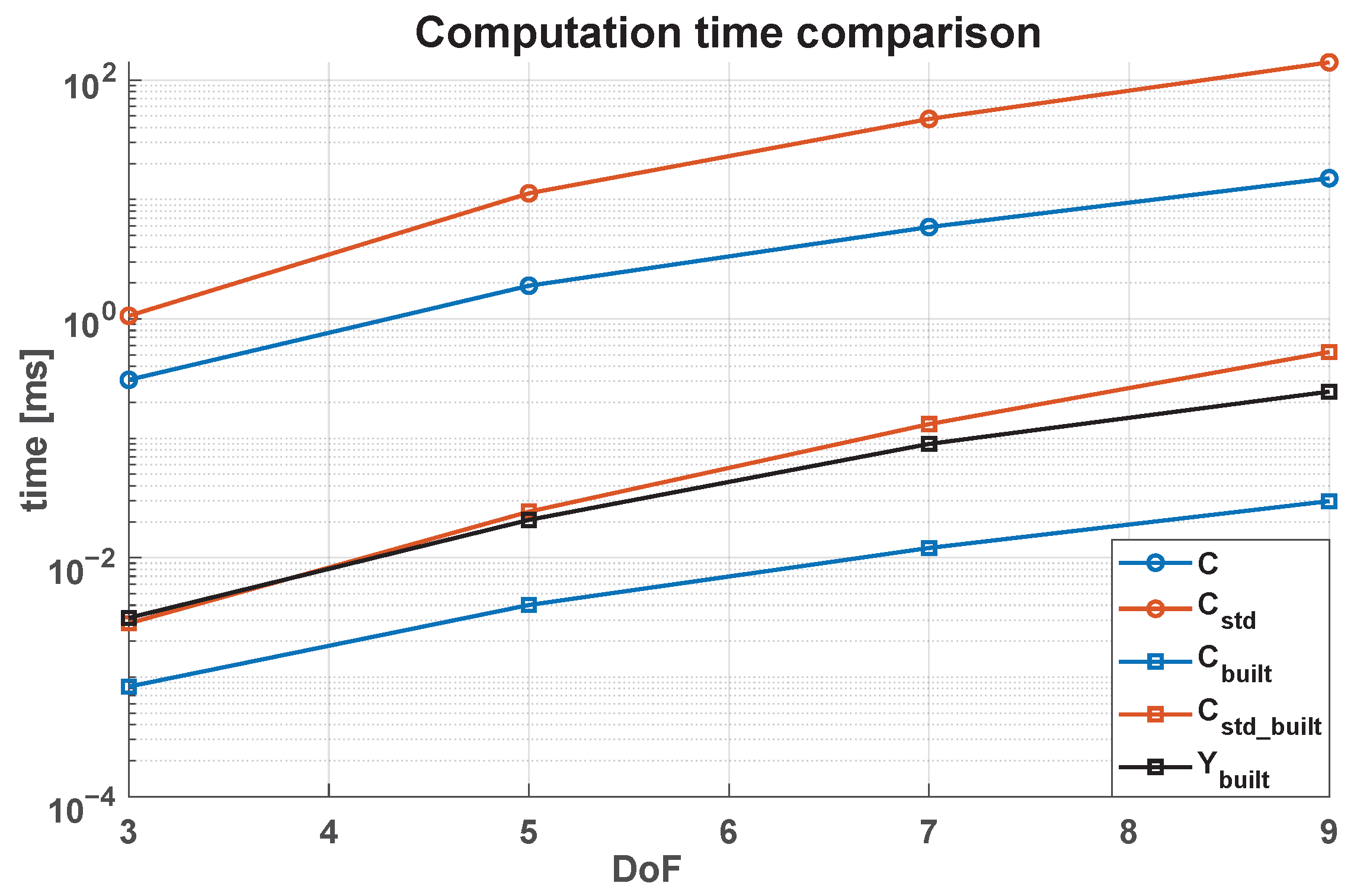
To evaluate the advantages of the new algorithm, we focus on the execution time as a comparison parameter. Figure 2 shows a comparisons of the time needed to compute the Coriolis matrix and the regressor for serial manipulators with different DoFs.

To perform this test, we used a PC with an 11th Gen Intel^® Core^TM i7-1165G7. The main difference between the algorithms is how the Coriolis terms are computed: “$C_{\mathrm{std}}$” uses the classic approach with Christoffel symbols, “C” uses the algorithm proposed in this paper, and the last three ($C_{\mathrm{built}}$, $C_{\mathrm{std}\_\mathrm{built}}$, $Y_{\mathrm{built}}$) are obtained from the C-code generation function, made available by CasADi, of the first two algorithms and the complete regressor matrix $Y_{\mathrm{r}}$.

As can be seen in Figure 2, our approach to computing the Coriolis matrix obtains computational times up to one order of magnitude below those of the classical method. This result leads to our approach obtaining a computational time for the whole regressor matrix $Y_{\mathrm{r}}$ that is lower than the one needed for $C_{\mathrm{std}}$ with the increase in of the number of DoFs involved. In our trials, we also show that our code is faster by more than two orders of magnitude w.r.t. the direct use of CasADi symbols. The time needed to create the symbolic robot and compute the standard quantities, and the time used to create the C++ library, are presented in

Table 2. Time comparison for the robot and library creation.

DoF	3	5	7	9	15	30
Robot creation [$\mathrm{ms}$]	23	81	326	954	5582	18,454
Library creation [$\mathrm{s}$]	$0.6$	$0.8$	$1.1$	$2.3$	$12.1$	$155.1$

.

We also compared our algorithm against the popular state-of-the-art library Pinocchio [7] and found that the execution times are of the same order of magnitude, in terms of computation, as a 7-DOF serial manipulator for the Jacobian J, its derivative $\dot{J}$, Coriolis matrix C, the mass matrix M, its derivative $\dot{M}$, and the regressor matrix. To determine the latter, since Pinocchio does not have the Slotine-Li formulation of the regressor $Y_{\mathrm{r}}(q,\dot{q},{\dot{q}}_{\mathrm{r}},{\ddot{q}}_{\mathrm{r}})$, we compare it with the standard $Y(q,\dot{q},\ddot{q})$. In addition to the average execution times, we also report jitter-related statistics (standard deviation and coefficient of variation) for our library, which quantify the variability of the execution time. The results show that the jitter remains limited (typically below $20\%$ CV), confirming the predictability of the library execution. A comparison of execution times is reported in

Table 3. Execution time statistics. The lowest values of computation time for each quantity are written in bold.

Library	J	$\dot{\mathit{J}}$	M	C	$\dot{\mathit{M}}$	Y
Our [$\mathrm{ns}$]	101	149	534	6003	1607	32,279
Our ($\sigma$)	21.3	7.6	22.1	697	74.0	1834
Our (CV [%])	21.2	4.4	4.2	12.0	4.6	6.1
Pinocchio [$\mathrm{ns}$]	402	908	969	3444	5774	5197

, where the values are presented in nanoseconds.

These results show that our library not only achieves competitive or superior average execution times compared to a state-of-the-art method, but also exhibits limited jitter, ensuring stable performance.

It is important to note that the purpose of these two libraries is different. Pinocchio offers a comprehensive set of tools for robot dynamics that users access directly. It also offers computations of kinematic/dynamic regressors for system identification, but it does not ship a ready-to-use Li–Slotine adaptive-control regressor (identification pipelines are typically handled via external toolboxes [26]). Thunder Dynamics focuses on adaptive control out-of-the-box. In particular, it exposes single-call APIs not only to common quantities, but also to adaptive-control regressors: the Li–Slotine-style regressor $Y_r$ and decomposed terms plus additional regressors (e.g., for $J\dot{q}$). Thunder also supports symbolic expressions for almost all dynamic and kinematic parameters, enabling runtime adaptation without recompilation. It also provides a lightweight extension mechanism to register custom functions or regressors that are compiled into the generated class. Our library is designed as a lightweight, self-contained class with minimal dependencies (the generated library requires Eigen and yaml-cpp) and a narrow API tailored to real-time adaptive control, which simplifies integration and deployment.

4. Adaptive Control Implementation

In this section, we show a complete control law, including position and orientation, for end-effector trajectory-tracking. The presented approach is based on the general theory of backstepping control reported in [32]. In the literature, various works exploit backstepping theory to develop adaptive task-space control for robotic manipulators. For example, in [33], the authors use the theory of backstepping to develop an adaptive control law to follow a position path in the Cartesian space with the end-effector of a mobile manipulator. A similar problem is studied in [34] for a parallel manipulator with a fixed base. In [35], the authors use an adaptive backstepping control for the position-tracking of a manipulator, taking the motor currents into consideration. However, none of them handle the Cartesian orientation of the end-effector. Here, our purpose is to provide a clean and complete implementation of an adaptive backstepping control for robotic manipulators. The obtained closed-loop system is also asymptotically stable in the presence of uncertainties in dynamical parameters. The complete scheme of the controller is depicted in Figure 3.

Consider a task where the goal is to follow a desired trajectory in Cartesian space defined by position and orientation. We define the error in pose $e\in {\mathbb{R}}^6$ as

$$e=\left[\begin{array}{c}{e}_{\mathrm{p}}\\ e_{\mathrm{o}}\end{array}\right]=\left[\begin{array}{c}{p}_{\mathrm{d}}-p\\ \mathrm{r}sin\left(\theta \right)\end{array}\right],$$

(27)

where $e_{\mathrm{p}}$, $e_{\mathrm{o}}\in {\mathbb{R}}^3$ are the error in position and orientation, respectively. The error in position is the difference between the desired position $p_{\mathrm{d}}\in {\mathbb{R}}^3$ and the linear part of the pose $p\in {\mathbb{R}}^3$ extracted by actual forward kinematics. The error in orientation exploits the axis-angle representation, $r\in {\mathbb{R}}^3$ and $\theta \in \mathbb{R}$, which is well known and described in detail in [36]. For the sake of clarity, we reported a sketch in Appendix E.

The definition of derivative of the error is straightforward, i.e.,

$$\begin{array}{cc}\hfill \dot{e}& =\left[\begin{array}{c}{\dot{e}}_{\mathrm{p}}\\ {\dot{e}}_{\mathrm{o}}\end{array}\right]=L^{\top }{\xi }_{\mathrm{d}}-LJ\dot{q},\hfill \end{array}$$

(28)

where ${\xi }_{\mathrm{d}}\triangleq {\left[{\dot{p}}_{\mathrm{d}}{\left(t\right)}^{\top }{\omega }_{\mathrm{d}}{\left(t\right)}^{\top }\right]}^{\top }\in {\mathbb{R}}^6$ is the desired end-effector twist, and matrix $L\in {\mathbb{R}}^{6\times 6}$ is the Jacobian transformation ensuring consistency with the error definition in (27):

$$L\triangleq \left[\begin{array}{cc}I& 0\\ 0& L_{\mathrm{o}}\end{array}\right],$$

(29)

where $L_{\mathrm{o}}$ is described in Appendix E.

The overall control problem can be divided into three steps: (i) kinematic control, (ii) dynamic control, and (iii) adaptive control. First, in Proposition 1, the design of a kinematic control law generates joint velocity references ${\dot{q}}_{\mathrm{r}}\in {\mathbb{R}}^n$ that ensure the end-effector position and orientation-tracking. Second, in Proposition 2, the dynamic control law generates the necessary joint torque command to follow the desired joint velocity computed by the kinematic part. Finally, the entire loop is closed, considering the inertial uncertainties in Proposition 3. This approach relies on four main assumptions: (1) there is perfect knowledge of the kinematic model of the manipulators; (2) the singular configuration of the manipulator during motion is avoided; (3) the parameters of the real system $\pi$ are constant over time; and (4) no external disturbance forces are applied on the manipulator. To increase readability, in the following, the dependence on joint position and its derivative is omitted when trivial.

Proposition 1 (Kinematic control asymptotic stability).

Consider the Cartesian pose error defined in (27) and the kinematics error model in (28). If joint velocities are as follows:

$$\dot{q}={\dot{q}}_{\mathrm{r}}\triangleq J^{†}{L}^{-1}\left(L^{\top }{\xi }_{\mathrm{d}}+\Lambda e\right),$$

(30)

where $\Lambda \in {\mathbb{R}}^{6\times 6}$ is a symmetric positive-definite matrix and $J^{†}$ is the Moore–Penrose inverse of the Jacobian matrix, the origin is an asymptotically stable (A.S.) equilibrium for the kinematic error dynamics (28).

Proof. 

See Appendix F.1.    □

For the dynamic part, we rewrite the control (4) using the new state coordinates $(e,s)$, where e and its dynamic are defined in (27) and (28), and

$$s\triangleq {\dot{q}}_{\mathrm{r}}-\dot{q},$$

(31)

with ${\dot{q}}_{\mathrm{r}}$ defined as in (30).

Proposition 2 (Dynamic control asymptotic stability).

Considering the state $(e,s)$, the torque control law

$$\tau ={\tau }^{*}\triangleq B{\ddot{q}}_{\mathrm{r}}+C{\dot{q}}_{\mathrm{r}}+G+K_{\mathrm{d}}s+J^{\top }{L}^{\top }{K}_{\mathrm{p}}e,$$

(32)

where $K_{\mathrm{d}}\in {\mathbb{R}}^{n\times n},K_{\mathrm{p}}\in {\mathbb{R}}^{6\times 6}$ are the controller gains, makes system A.S. in the origin.

Proof. 

See Appendix F.2.    □

Proposition 3 (Uncertainties in the dynamic part).

Let $\widehat{\pi }$ be an estimate of the real inertial parameters π, and define $\tilde{\pi }\left(t\right)=\pi -\widehat{\pi }\left(t\right)$ as the parameters’ error. Moreover, let the estimated dynamical matrices be $(\widehat{B},\widehat{C},\widehat{G})$, obtained by computing the Euler–Lagrange equation using $\widehat{\pi }$ instead of the real parameters π. The control action

$$\tau =\widehat{B}{\ddot{q}}_{\mathrm{r}}+\widehat{C}{\dot{q}}_{\mathrm{r}}+\widehat{G}+K_{\mathrm{d}}s+J^{\top }{L}^{\top }{K_{\mathrm{p}}}^{\top }e,$$

(33)

where $K_{\mathrm{d}}\in {\mathbb{R}}^{n\times n},K_{\mathrm{p}}\in {\mathbb{R}}^{6\times 6}$ are the controller gains, and the parameter update law

$$\dot{\widehat{\pi }}=u_{\pi }\triangleq {\Gamma }^{-1}{Y_{\mathrm{r}}}^{\top }s,$$

(34)

where $Y_{\mathrm{r}}=Y_{\mathrm{r}}(q,\dot{q},{\dot{q}}_{\mathrm{r}},{\ddot{q}}_{\mathrm{r}})$ is defined as (6), and Γ is a positive-definite gain matrix, leading to asymptotic stability in the closed-loop system.

Proof. 

See Appendix F.3.    □

Remark 1. 

The control law (33) is similar to the one in [11], as it only differs in the term $J^{\top }{L}^{\top }{K_{\mathrm{p}}}^{\top }e$, which introduces a term proportional to the tracking error. We also explicitly include the inverse kinematic solution in the overall closed loop. The advantage of this inclusion is that it ensures the asymptotic stability of end-effector tracking, as opposed to the case when the adaptive controller tracks the solution in the joint space provided by a separate external inverse kinematic solver. In this sense, it is possible to view adaptive backstepping as a slight generalization of the classical adaptive control techniques mainly used in the literature. Finally, it should be mentioned that, in case there is also uncertainty in the kinematic parameters entering the kinematic system (e.g., in the Jacobian entries), the backstepping controller design procedure would still apply through the addition of a fourth Lyapunov function between the first and second stages, basically following [37]. Details are omitted here for brevity.

Remark 2. 

In the case that not all parameters contain uncertainties, it is possible to split the Equation (5) into known ($Y_{\mathrm{k}}{\pi }_{\mathrm{k}}$) and unknown ($Y_{\mathrm{u}}{\pi }_{\mathrm{u}}$) parts, and reduce the number of symbolic parameters. However, the resulting equation is no longer linear for the unknown parameters ${\pi }_{\mathrm{u}}$. A possible solution could be adding 1 to the new parameters representing the known dynamics, i.e.,

$$\tau =Y_{\mathrm{k}}{\pi }_{\mathrm{dk}}+Y_{\mathrm{u}}{\pi }_{\mathrm{u}}=\left[\begin{array}{cc}{Y}_{\mathrm{k}}{\pi }_{\mathrm{dk}}& Y_{\mathrm{u}}\end{array}\right]\left[\begin{array}{c}1\\ {\pi }_{\mathrm{du}}\end{array}\right]$$

(35)

This method is used in Thunder Dynamics to obtain symbolic selectivity and improve performance when a parameter is perfectly known.

Remark 3. 

While the proposed control law permits ${lim}_{t\to \infty }e\left(t\right)=0$ and ${lim}_{t\to \infty }\dot{e}\left(t\right)=0$ to be obtained, it is not possible to draw conclusions regarding the convergence of the estimated inertia parameters $\tilde{\pi }$ to the real value π. This is for two principal reasons: the structural observability of these parameters from the manipulator’s dynamic equation and the persistent excitation of the trajectory performed. The classical representation of the serial kinematic chain’s inertia relies on the parametrisation of the inertia of rigid bodies, which consists of 10 parameters (one for the mass, three for the center-of-mass position, and six for the inertia tensor). The manipulator’s inertia is represented by the union of the inertia parameters of each link. However, this choice leads to a set of parameters that are not fully observable in terms of the joint torques. Several works discuss the problem of overparametrization [38], like the identification of minimum sets of parameters [39] or the definition of estimation procedures for complex kinematic chains [40]. From this point of view, the structure of our tool allows the user to easily add new functions. Thanks to this, the user can implement solutions like the one proposed in [39] and deal with overparametrization. The other aspect of parameter estimation is related to the motion performed by the system. In fact, to obtain a reliable estimation, the parameters should be excited in a proper way. This concept is called Persistent Excitation (PE) [41,42], and it is verified if $l_0,l_1,l_2$ exists, such that

$$\forall t<0,l_{1}I\le {\int }_t^{t+l_0}{Y}^{\top }\left(r\right)Y\left(r\right)dr\le l_{2}I.$$

For the sake of clarity, we briefly report, in

Table 4. Overall control law.

Variable	Definition	Reference
e	$\left[\begin{array}{c}{e}_p\\ e_o\end{array}\right]=\left[\begin{array}{c}{p}_d-p\\ rsin\theta \end{array}\right]$	(27)
${\dot{q}}_{\mathrm{r}}$	$J^{†}{L}^{-1}\left(L^{\top }{\xi }_{\mathrm{d}}+\Lambda e\right)$	(30)
s	${\dot{q}}_{\mathrm{r}}-\dot{q}$	(31)
$\tau$	$\widehat{B}{\ddot{q}}_{\mathrm{r}}+\widehat{C}{\dot{q}}_{\mathrm{r}}+\widehat{G}+K_{\mathrm{d}}s+J^{\top }{L}^{\top }{K_{\mathrm{p}}}^{\top }e$	(33)
$u_{\pi }$	$R{Y}^{\top }s$	(34)

, all the key components of the proposed control law.

5. Experimental Validation

In this section, we validate the usage of Thunder Dynamics in implementing adaptive control on real manipulators. To test our approach, we exploited the library developed in this work to design a ROS package for adaptive control. This software package was developed for Franka Emika Panda manipulator and it is available online in the adaptive branch of the repository panda_controllers (https://github.com/CentroEPiaggio/panda_controllers, accessed on 10 September 2025). The code generated by the new algorithm proposed in this paper satisfies the strict constraints of real-time scheduling, which requires the control loop frequency to be 1 $\mathrm{kHz}$.

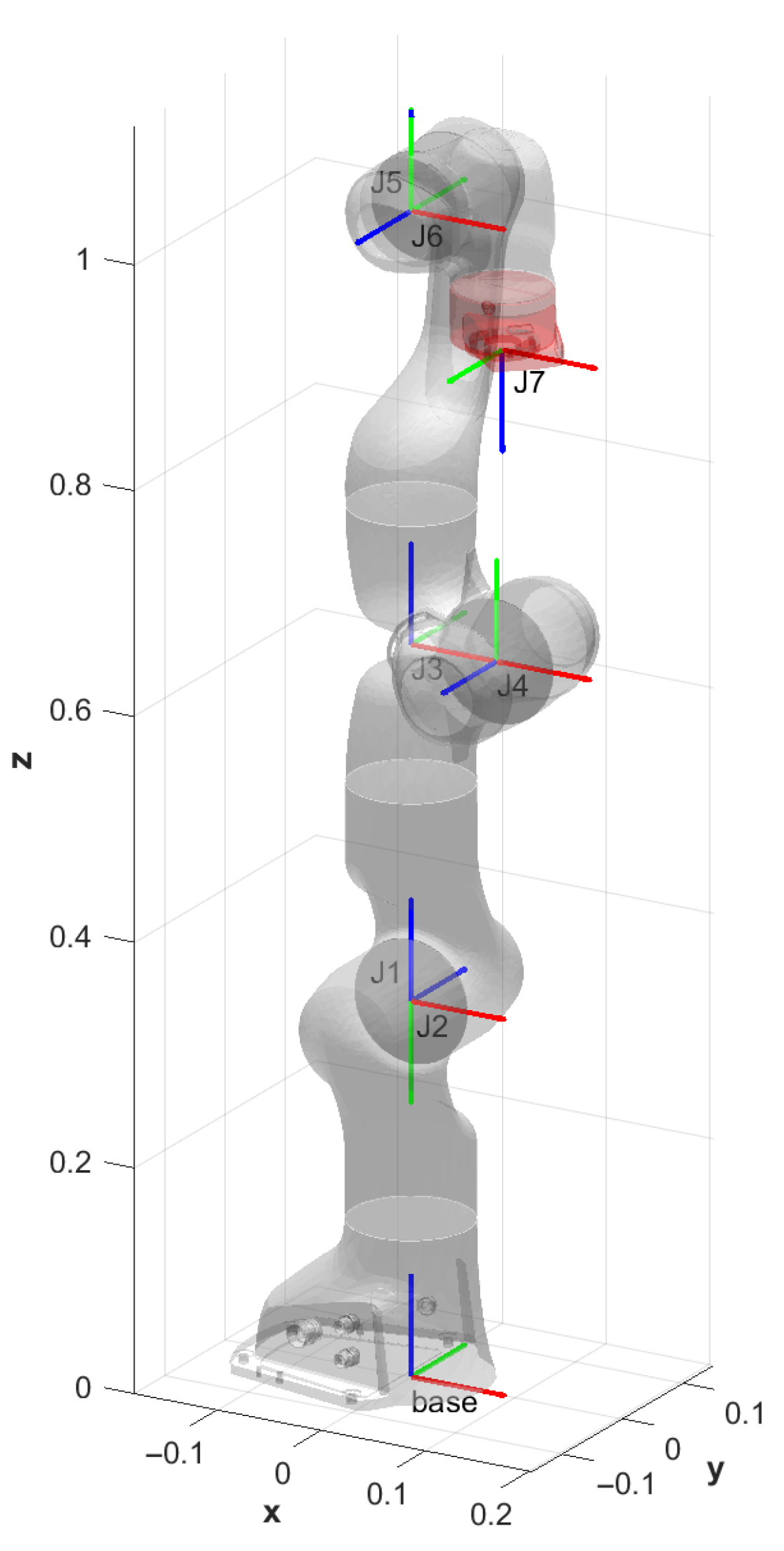
Figure 4 shows how the frames of each link are chosen in agreement with DH rules, and the related DH table is provided in

Table 5. Denavit-Hartenberg Table.

Linki	${\mathit{a}}_{\mathit{i}}$	${\mathit{\alpha }}_{\mathit{i}}$	${\mathit{d}}_{\mathit{i}}$	${\mathit{\theta }}_{\mathit{i}}$
1	0	0	0.3330	$q_1$
2	0	−$\pi /2$	0	$q_2$
3	0	$\pi /2$	0.3160	$q_3$
4	0.0825	$\pi /2$	0	$q_4$
5	−0.0825	−$\pi /2$	0.384	$q_5$
6	0	$\pi /2$	0	$q_6$
7	0.088	$\pi /2$	0.107	$q_7$

. The dimensions of the robot and its parameters are provided by Franka Control Interface (https://frankarobotics.github.io/docs/control_parameters.html, accessed on 10 September 2025).

In addition to presenting an example of the implementation of the adaptive controller using Thunder Dynamics, in this section, we provide a full characterization of the controller behaviour. The tests were performed both in simulation, using the robot model provided by Franka in the Gazebo simulator [43], and on the real hardware, to test its effectiveness in meeting the computational constraints of the robotic system.

In all the tests we carried out, we generated the reference trajectory exploiting Lissajous, a family of parametric curves defined as follows:

$$p_{\mathrm{d}}\left(t\right)=\left(\begin{array}{c}Asin\left(2\pi a(t-t_0)\right)\\ Bcos\left(2\pi b(t-t_0)\right)\\ Csin\left(2\pi c(t-t_0)\right)\end{array}\right)+\left(\begin{array}{c}{x}_0\\ y_0\\ z_0\end{array}\right)$$

where, in our work, $A=0.10\mathrm{m}$, $B=0.15\mathrm{m}$, $C=0.1\mathrm{m}$, $a=0.20\mathrm{Hz}$, $b=0.10\mathrm{Hz}$, and $c=0.40\mathrm{Hz}$, obtaining the trajectory depicted in Figure 5 and keeping the Cartesian orientation constant.

Even if this trajectory did not meet the criteria of PE, we chose to use it for the experimental validation because it permitted us to show the effectiveness of the implementation of the adaptive control law using the tool proposed in our manuscript, discussing the different behaviours of the manipulator obtained through different sets of gains.

For the controller setup, we used the following matrix gains:

$$\begin{array}{cc}\hfill & \Lambda =\mathrm{diag}\left({\lambda }_1,\dots ,{\lambda }_6\right),\hfill \\ \hfill & K_{\mathrm{d}}=\mathrm{diag}\left(k_{\mathrm{d}1},\dots ,k_{\mathrm{d}7}\right),\hfill \\ \hfill & \Gamma =\mathrm{diag}\left({\Gamma }_1,\dots ,{\Gamma }_7\right),\hfill \\ \hfill & {\Gamma }_i=r_i·\mathrm{diag}\left(r_{\mathrm{m}},r_{c1},\dots ,r_{\mathrm{c}3},r_{\mathrm{I}1},\dots ,r_{\mathrm{I}6}\right)\hfill \end{array}$$

(36)

where ($r_{\mathrm{m}},r_{\mathrm{c}},r_{\mathrm{I}}$) are the gains for mass, centers of mass, and inertia tensor parameters, respectively.

5.1. Simulation Tests

The first step of validation was performed in a simulated environment. During this phase, we tested how the performance of the controller changes with respect to the values assigned to $K_{\mathrm{d}}$ and $\Gamma$. For each matrix gain, we chose three sets of values, which permitted us to better explain the behaviour of the control law. To reproduce a case where there are uncertainties in the inertial parameters, we introduced an error in the internal dynamic model of the controller. To maximize the effect in terms, the model error was introduced in the last link, setting a mass m = $2.5$ kg and a Center of Mass $CoM$ = (20, 20, 20) cm, while the real values, provided by the manufacturer, were equal to m = $0.73$ kg, $CoM$ = ($1.05$, $-0.43$, $-4.52$) cm. Regarding inertial tensor terms, we set them as equal to zero in the model. Given the negligible effect on the tracking error they had in this case with respect to the other parameters, we omit the discussion about them in the following.

First, we discuss the choice of gain $K_{\mathrm{d}}$. As we can observe in Figure 6, while the temporal behaviours of the tracking error over time are similar with different gains, the main effect is related to its initial amplitude. This is because a higher gain leads to a controlled system that is less sensitive to inertial parameter errors. This is also confirmed by the steady state error and rise time reported in

Table 6. Steady-state and rise time values of tracking errors for different values of $K_{\mathrm{d}}$.

	Kd1	Kd2	Kd3
Steady-state error	0.0258	0.0219	0.0226
Rise time [$\mathrm{s}$]	15.102	19.612	15.961

. Moving instead to inertial parameter convergence (Figure 7), we can observe that lower values of $K_{\mathrm{d}}$ lead to their faster convergence. The reason behind this behavior is that the parameter’s update rate is strictly connected with the tracking error, and if the error decreases too quickly, the update law slows down sooner and requires more time to converge. In those cases, the selection of a more exciting trajectory could help achieve convergence. This concept is clearly shown by the behaviour of component z of the estimated CoM. For the trajectory used in this work, this component is always aligned with the gravity, leading to a small effect on the following trajectory and, consequently, to smaller changes in the estimate.

Following this, we move to a discussion on the effect of $\Gamma$ on the system’s behavior. In Figure 8, the tracking error convergence achieved with different values is depicted. As we can observe, higher values of $\Gamma$ lead to slower tracking convergence. This is because the update law is proportional to ${\Gamma }^{-1}$, and the controlled system needs more time to adapt the inertial model to the real system. This slower convergence is also shown in Figure 9. However, it is evident from the plot that if we decrease $\Gamma$ too much, undesired oscillatory behavior in the parameter estimation appears, leading to the conclusion that it is not convenient to arbitrarily decrease $\Gamma$. In

Table 7. Steady-state and rise time values of tracking error for different values of $\Gamma$.

	${\mathit{r}}_7=1$	${\mathit{r}}_7=10$	${\mathit{r}}_7=100$
Steady-state error	0.0136	0.0219	0.1204
Rise time [$\mathrm{s}$]	3.668	19.612	23.572

, the steady state and rise time values for the tracking error with the different values of $\Gamma$ are reported.

5.2. Real Manipulator Tests

After simulations, we moved to the controller’s implementation on a real manipulator. This provided results regarding the implementation of adaptive control, and allowed us to check if the generated library satisfies the requirements of a real manipulator. We implemented two versions of the Backstepping control on the manipulator—the classical version and the adaptive one—maintaining the same set of gains to check the improvements provided by the adaptive law. Figure 10 represents the tracking error of the two controllers under the same conditions. The results show that, while the non-adaptive control achieves a time-varying error of around $0.9$ (strictly depending on the actual state of the robot and how much the dynamic model error affects the tracking), the adaptive control converges to a tracking error that is an order of magnitude below this, handling the dynamic uncertainties in the model of the manipulator. This result in terms of the tracking error obtained on the real manipulator is also comparable with the ones obtained in the simulation tests, confirming the effectiveness of this approach on real hardware.

As the last experiment, a SoftHand [44] was fixed to the robot’s flange (Figure 11), and the adaptive control law was only used on link 7. In this case, the inertial parameters of the SoftHand were not considered in the model. This test aims to verify the correct tracking with the adaptive controller if an unidentified object is fixed on the end-effector.

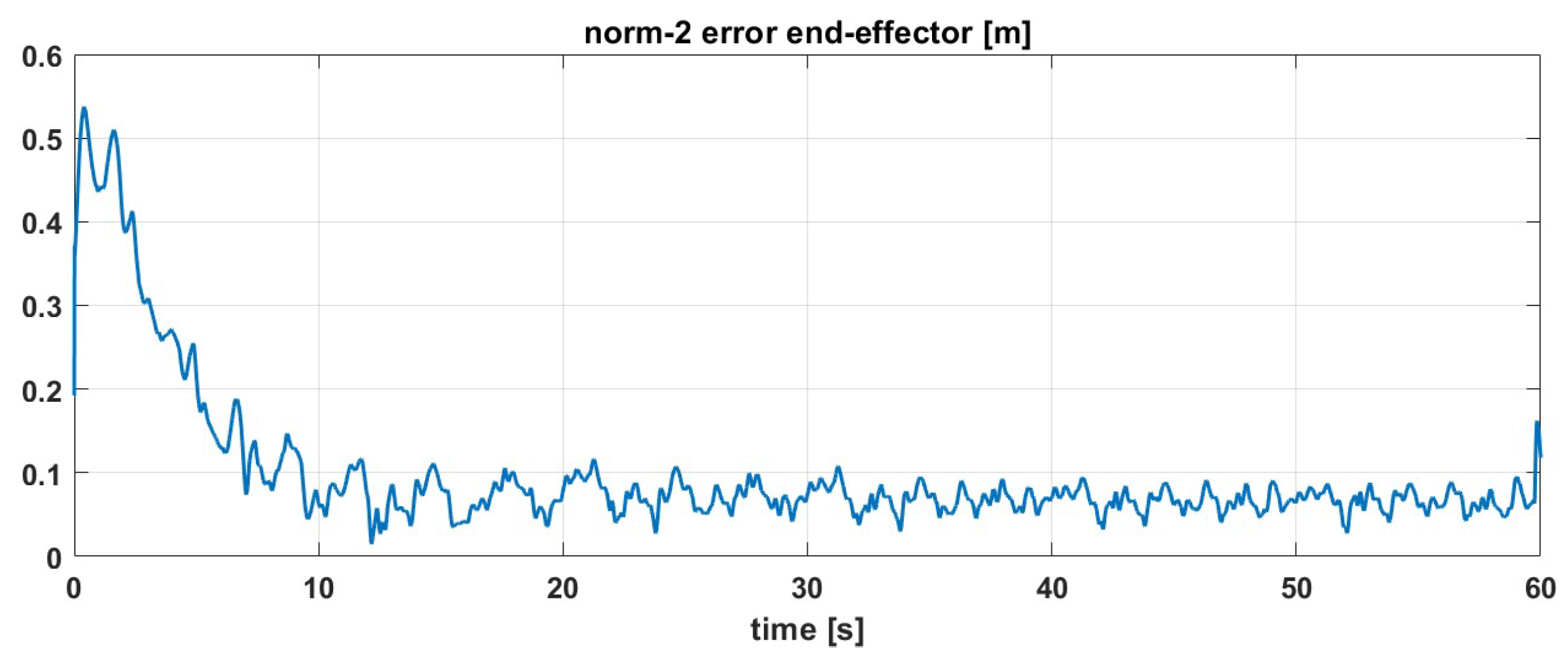
Figure 12 and Figure 13 show the tracking error and the inertial parameter estimation, respectively. We can see that the tracking error stabilises its values at around $t=10\mathrm{s}$. This is consistent with the temporal behaviour of the estimated inertial parameters, where the estimated mass, which is the term that usually has more effect on the dynamics of classical manipulators, simultaneously achieves values near the true value. This proves the adaptive controller’s ability to compensate for disturbances related to the unknown inertial parameters of the end-effector. For the sake of completeness, we also report the comparison between the true values and the estimated ones in

Table 8. Estimation of Softhand + Link 7 parameters in $\left\{S_7\right\}$.

	Mass [kg]	CoMx [m]	CoMy [m]	CoMz [m]
True	1.5655	0.06170	−0.0004	0.0009
Estimate	1.7542	0.0414	−0.0039	−0.0191
Initial	0.736	0.014	−0.004	−0.045

. True values were computed using the inertial parameters provided by the manufacturer (https://qbrobotics.com/product/qb-softhand-research, accessed on 10 September 2025) and merging these with the inertial parameters of link 7 of the manipulator using the Huygens–Steiner theorem. As we can see, adaptive control reduces the error between real and estimated parameters. However, the final error in some of these parameters continues to be non-negligible. The main reason behind this result can be found in the concepts explained in Remark 3 regarding the observability of the parameters. Furthermore, the proposed control law is designed to provide asymptotic stability in terms of trajectory-tracking error, while nothing can be said about the convergence of the estimated inertial parameters to the real values. Other adaptive control law formulations have been proposed in the literature, which provide stronger results in terms of parameter estimation [45]. However, this is out of the scope of this manuscript.

6. Discussion and Conclusions

Adaptive controllers are a family of controllers that are able to compensate for errors in the dynamic model of the controlled system. While these controllers are very effective in minimizing tracking errors due to incorrect inertial parameters, they require the factorization of the dynamic equation of the system. Previous work provided a theoretical solution for this step [21]. However, it suffers from practical limitations hindering its direct deployment in real-time systems with multiple DoFs.

In our work, we presented a novel formulation of this approach that can be easily integrated into the classical software structure used for the control of real robot manipulators. This algorithm was then applied in the development of a software library, Thunder Dynamics, to provide all the necessary information to implement adaptive control in a robotic serial manipulator. To demonstrate the effectiveness of our software, we implemented an adaptive controller for a 7-DoF manipulator. Specifically, we developed a task-space backstepping control approach tailored for robotic manipulators. The entire framework was evaluated on real hardware, showing that our solution enables the design of adaptive controllers capable of handling dynamic model errors during trajectory-tracking. Both the software tool and the ROS controller have been released and are freely available online.

Starting from these results, there are different possible future developments to increase the range of application of this library. A next step is to broaden the range of kinematic architectures supported by the framework, notably floating-base systems and mechanisms with closed kinematic loops. This requires, for example, augmenting the state to add the floating-base state, implementing Jacobian contact support, and adopting a floating-base dynamics formulation [46].

Another point to be tackled is the possibility of adding other types of parameters that can be parametrized beyond the classical inertial ones. Inertial properties are not the only factors that influence the dynamic behavior of robots. Friction, as pointed out by [47], could have a great impact on the system. In one of our latest works, we tested a simple implementation of the joint friction model using our library [48]. As future work, we plan to incorporate a more advanced and accurate representation of friction within the system. Moreover, geometrical quantities can also be formalized to directly construct a kinematic regressor matrix. If the control algorithm does not have perfect knowledge of these, they could be changed online to increase the controller’s performance.

Given the structure of the proposed tool, the generated library is also suitable for use in embedded systems. Indeed, for robots with a small number of DOFs (namely $\le 4$), the generated files are compact enough to be cross-compiled for microcontrollers. It will be important to explore and test this application, since the complexity of newer controller tools is constantly increasing.

References

1. Evjemo, L.D.; Moe, S.; Gravdahl, J.T.; Roulet-Dubonnet, O.; Gellein, L.T.; Br, V. Additive manufacturing by robot manipulator: An overview of the state-of-the-art and proof-of-concept results. In Proceedings of the 2017 22nd IEEE International Conference on Emerging Technologies and Factory Automation (ETFA), Limassol, Cyprus, 12–15 September 2017; pp. 1–8. [Google Scholar]
2. Ghodsian, N.; Benfriha, K.; Olabi, A.; Gopinath, V.; Arnou, A. Mobile Manipulators in Industry 4.0: A Review of Developments for Industrial Applications. Sensors 2023, 23, 8026. [Google Scholar] [CrossRef]
3. Kim, J.; Gu, G.M.; Heo, P. Robotics for healthcare. In Biomedical Engineering: Frontier Research and Converging Technologies; Springer: Cham, Switzerland, 2016; pp. 489–509. [Google Scholar]
4. Featherstone, R.; Orin, D.E. Dynamics. In Springer Handbook of Robotics; Springer: Cham, Switzerland, 2016; pp. 37–63. [Google Scholar]
5. Featherstone, R. Rigid Body Dynamics Algorithms; Springer: Berlin/Heidelberg, Germany, 2014. [Google Scholar]
6. Felis, M.L. RBDL: An efficient rigid-body dynamics library using recursive algorithms. Auton. Robot. 2017, 41, 495–511. [Google Scholar] [CrossRef]
7. Carpentier, J.; Saurel, G.; Buondonno, G.; Mirabel, J.; Lamiraux, F.; Stasse, O.; Mansard, N. The Pinocchio C++ library: A fast and flexible implementation of rigid body dynamics algorithms and their analytical derivatives. In Proceedings of the 2019 IEEE/SICE International Symposium on System Integration (SII), Paris, France, 14–16 January 2019; pp. 614–619. [Google Scholar]
8. Leboutet, Q.; Roux, J.; Janot, A.; Guadarrama-Olvera, J.R.; Cheng, G. Inertial parameter identification in robotics: A survey. Appl. Sci. 2021, 11, 4303. [Google Scholar] [CrossRef]
9. Hsia, T. Adaptive control of robot manipulators-a review. In Proceedings of the 1986 IEEE International Conference on Robotics and Automation, San Francisco, CA, USA, 7–10 April 1986; Volume 3, pp. 183–189. [Google Scholar]
10. Zhang, D.; Wei, B. A review on model reference adaptive control of robotic manipulators. Annu. Rev. Control 2017, 43, 188–198. [Google Scholar] [CrossRef]
11. Slotine, J.J.E.; Li, W. On the adaptive control of robot manipulators. Int. J. Robot. Res. 1987, 6, 49–59. [Google Scholar] [CrossRef]
12. Harandi, M.R.J.; Hassani, A.; Hosseini, M.I.; Taghirad, H.D. Adaptive Position Feedback Control of Parallel Robots in the Presence of Kinematics and Dynamics Uncertainties. IEEE Trans. Autom. Sci. Eng. 2024, 21, 989–999. [Google Scholar] [CrossRef]
13. Liu, Z.; Zhao, Y.; Zhang, O.; Chen, W.; Wang, J.; Gao, Y.; Liu, J. A Novel Faster Fixed-Time Adaptive Control for Robotic Systems With Input Saturation. IEEE Trans. Ind. Electron. 2024, 71, 5215–5223. [Google Scholar] [CrossRef]
14. Piao, J.; Kim, M.C.; Kim, E.S.; Kim, C.S. A Self-Adaptive Inertia Hybrid Control of a Fully Constrained Cable-Driven Parallel Robot. IEEE Trans. Autom. Sci. Eng. 2024, 21, 2063–2073. [Google Scholar] [CrossRef]
15. Zhang, B.; Shang, W.; Deng, B.; Cong, S.; Li, Z. High-Precision Adaptive Control of Cable-Driven Parallel Robots with Convergence Guarantee. IEEE Trans. Ind. Electron. 2024, 71, 7370–7380. [Google Scholar] [CrossRef]
16. Le, D.M.; Patil, O.S.; Amy, P.M.; Dixon, W.E. Integral concurrent learning-based accelerated gradient adaptive control of uncertain Euler-Lagrange systems. In Proceedings of the 2022 American Control Conference (ACC), Atlanta, GA, USA, 8–10 June 2022; pp. 806–811. [Google Scholar]
17. Liu, Y.; Teng, L.; Jin, Z. Adaptive control of mini space robot based on linear separation of inertial parameters. Aerospace 2023, 10, 679. [Google Scholar] [CrossRef]
18. Chen, Y.; Ding, J.; Chen, Y.; Yan, D. Nonlinear robust adaptive control of universal manipulators based on desired trajectory. Appl. Sci. 2024, 14, 2219. [Google Scholar] [CrossRef]
19. Khosla, P.K.; Kanade, T. Parameter identification of robot dynamics. In Proceedings of the 1985 24th IEEE Conference on Decision and Control, Fort Lauderdale, FL, USA, 11–13 December 1985; pp. 1754–1760. [Google Scholar] [CrossRef]
20. Garofalo, G.; Ott, C.; Albu-Schäffer, A. On the closed form computation of the dynamic matrices and their differentiations. In Proceedings of the 2013 IEEE/RSJ International Conference on Intelligent Robots and Systems, Tokyo, Japan, 3–7 November 2013; p. 2364-2359. [Google Scholar] [CrossRef]
21. Gabiccini, M.; Bracci, A.; De Carli, D.; Fredianelli, M.; Bicchi, A. Explicit Lagrangian formulation of the dynamic regressors for serial manipulators. In Proceedings of the XIX Aimeta Congress, Ancona, Italy, 14–19 September 2009; pp. 14–17. [Google Scholar]
22. Denavit, J.; Hartenberg, R.S. A kinematic notation for lower-pair mechanisms based on matrices. J. Appl. Mech. 1955, 22, 215–221. [Google Scholar] [CrossRef]
23. Nori, F.; Traversaro, S.; Eljaik, J.; Romano, F.; Del Prete, A.; Pucci, D. iCub whole-body control through force regulation on rigid non-coplanar contacts. Front. Robot. AI 2015, 2, 6. [Google Scholar] [CrossRef]
24. Mastalli, C.; Budhiraja, R.; Merkt, W.; Saurel, G.; Hammoud, B.; Naveau, M.; Carpentier, J.; Righetti, L.; Vijayakumar, S.; Mansard, N. Crocoddyl: An Efficient and Versatile Framework for Multi-Contact Optimal Control. In Proceedings of the IEEE International Conference on Robotics and Automation (ICRA), Paris, France, 31 May–31 August 2020. [Google Scholar]
25. Developers, A. ADAM: Automatic Differentiation for Rigid-Body-Dynamics AlgorithMs. 2023. Available online: https://github.com/ami-iit/ADAM (accessed on 10 September 2025).
26. Nguyen, D.V.T.; Bonnet, V.; Maxime, S.; Gautier, M.; Fernbach, P.; Lamiraux, F. FIGAROH: A Python toolbox for dynamic identification and geometric calibration of robots and humans. In Proceedings of the 2023 IEEE-RAS 22nd International Conference on Humanoid Robots (Humanoids), Austin, TX, USA, 12–14 December 2023. [Google Scholar] [CrossRef]
27. Rickert, M.; Gaschler, A. Robotics library: An object-oriented approach to robot applications. In Proceedings of the 2017 IEEE/RSJ International Conference on Intelligent Robots and Systems (IROS), Vancouver, BC, Canada, 24–28 September 2017; pp. 733–740. [Google Scholar]
28. Corke, P.; Haviland, J. Not your grandmother’s toolbox–The robotics toolbox reinvented for python. In Proceedings of the 2021 IEEE International Conference on Robotics and Automation (ICRA), Xi’an, China, 30 May–5 June 2021; pp. 11357–11363. [Google Scholar]
29. Andersson, J.A.E.; Gillis, J.; Horn, G.; Rawlings, J.B.; Diehl, M. CasADi—A software framework for nonlinear optimization and optimal control. Math. Program. Comput. 2018, 11, 1–36. [Google Scholar] [CrossRef]
30. Gabiccini, M.; Bracci, A.; Artoni, A. Direct derivation of the dynamic regressors for serial manipulators with mixed rigidelastic joints. In Proceedings of the AttiXX Congresso dell’Associazione Italiana di Meccanica Teorica e Applicata, Bologna, Italy, 12–15 September 2011. [Google Scholar]
31. Boettiger, C. An introduction to Docker for reproducible research. Acm Sigops Oper. Syst. Rev. 2015, 49, 71–79. [Google Scholar] [CrossRef]
32. Krstic, M.; Kanellakopoulos, I.; Kokotovic, P.V. Nonlinear and Adaptive Control Design; Wiley: Hoboken, NJ, USA, 1995. [Google Scholar]
33. Patel, B.; Pan, Y.J.; Ahmad, U. Adaptive backstepping control approach for the trajectory tracking of mobile manipulators. In Proceedings of the 2017 IEEE International Conference on Robotics and Biomimetics (ROBIO), Macau, China, 5–8 December 2017; pp. 1769–1774. [Google Scholar] [CrossRef]
34. Zou, J.; Schueller, J. Adaptive backstepping control for parallel robot with uncertainties in dynamics and kinematics. Robotica 2014, 32, 1–24. [Google Scholar] [CrossRef]
35. Nganga-Kouya, D.; Saad, M.; Lamarche, L.; Khairallah, C. Backstepping adaptive position control for robotic manipulators. In Proceedings of the 2001 American Control Conference, (Cat. No.01CH37148), Arlington, VA, USA, 25–27 June 2001; Volume 1, pp. 636–640. [Google Scholar] [CrossRef]
36. Siciliano, B.; Sciavicco, L.; Villani, L.; Oriolo, G. Robotics: Modelling, Planning and Control; Advanced Textbooks in Control and Signal Processing; Springer: London, UK, 2010; pp. 105–160. [Google Scholar]
37. Cheah, C.; Liu, C.; Slotine, J. Adaptive Jacobian tracking control of robots with uncertainties in kinematic, dynamic and actuator models. IEEE Trans. Autom. Control 2006, 51, 1024–1029. [Google Scholar] [CrossRef]
38. Ortega, R.; Gromov, V.; Nuño, E.; Pyrkin, A.; Romero, J.G. Parameter estimation of nonlinearly parameterized regressions without overparameterization: Application to adaptive control. Automatica 2021, 127, 109544. [Google Scholar] [CrossRef]
39. Gautier, M.; Khalil, W. Direct calculation of minimum set of inertial parameters of serial robots. IEEE Trans. Robot. Autom. 1990, 6, 368–373. [Google Scholar] [CrossRef]
40. Bonnet, V.; Fraisse, P.; Crosnier, A.; Gautier, M.; González, A.; Venture, G. Optimal exciting dance for identifying inertial parameters of an anthropomorphic structure. IEEE Trans. Robot. 2016, 32, 823–836. [Google Scholar] [CrossRef]
41. Slotine, J.j.E.; Li, W. Adaptive robot control: A new perspective. In Proceedings of the 26th IEEE Conference on Decision and Control, Los Angeles, CA, USA, 9–11 December 1987; Volume 26, pp. 192–198. [Google Scholar] [CrossRef]
42. Slotine, J.J.E.; Li, W. Composite adaptive control of robot manipulators. Automatica 1989, 25, 509–519. [Google Scholar] [CrossRef]
43. Koenig, N.; Howard, A. Design and use paradigms for gazebo, an open-source multi-robot simulator. In Proceedings of the 2004 IEEE/RSJ International Conference on Intelligent Robots and Systems (IROS), Sendai, Japan, 28 September–2 October 2004; Volume 3, pp. 2149–2154. [Google Scholar]
44. Catalano, M.G.; Grioli, G.; Farnioli, E.; Serio, A.; Piazza, C.; Bicchi, A. Adaptive synergies for the design and control of the Pisa/IIT SoftHand. Int. J. Robot. Res. 2014, 33, 768–782. [Google Scholar] [CrossRef]
45. Obuz, S.; Tatlicioglu, E.; Zergeroglu, E. Adaptive Cartesian space control of robotic manipulators: A concurrent learning based approach. J. Frankl. Inst. 2024, 361, 106701. [Google Scholar] [CrossRef]
46. Traversaro, S.; Pucci, D.; Nori, F. A Unified View of the Equations of Motion Used for Control Design of Humanoid Robots. 2017. Available online: https://www.researchgate.net/publication/312200239_A_Unified_View_of_the_Equations_of_Motion_used_for_Control_Design_of_Humanoid_Robots (accessed on 10 September 2025).
47. Bona, B.; Indri, M. Friction Compensation in Robotics: An Overview. In Proceedings of the 44th IEEE Conference on Decision and Control, and the European Control Conference, Seville, Spain, 12–15 December 2005; Volume 2005, pp. 4360–4367. [Google Scholar] [CrossRef]
48. Simonini, G.; Baracca, M.; Cavaliere, T.V.; Bicchi, A.; Salaris, P. A Novel Formulation for Adaptive Computed Torque Control Enabling Low Feedback Gains in Highly Dynamical Tasks. IEEE Access 2025, 13, 69898–69909. [Google Scholar] [CrossRef]
49. Waldron, K.J.; Schmiedeler, J. Kinematics. In Springer Handbook of Robotics; Springer: Cham, Switzerland, 2016; pp. 12–21. [Google Scholar]
50. Khalil, H. Lyapunov Stability. In Nonlinear Systems; Pearson Education, Prentice Hall: Upper Saddle River, NJ, USA, 2002; pp. 111–181. [Google Scholar]
51. Khalil, H. Invariance-like Theorems. In Nonlinear Systems; Pearson Education, Prentice Hall: Upper Saddle River, NJ, USA, 2002; pp. 322–329. [Google Scholar]
Figure 1. Simplified UML diagram of the framework. The main program takes a configuration file as input, creates the robot, and fills it with functions, both default (kinematics, dynamics) and user-defined. The resulting object is then included in a C++ library.
Robotics 14 00126 g001
Figure 2. Execution time comparison of different algorithms. Our algorithm is generally faster and permits the real-time adaptive control of a 7-DoF manipulator.
Robotics 14 00126 g002
Figure 3. Overall scheme of the Adaptive Backstepping Control. The desired Cartesian trajectory serves as the input to the Inverse Kinematics block, which generates new joint references and new coordinates. These outputs are utilized by the Adaptive Law block for updating inertial parameters and by the Control block to ensure asymptotic stability. The Plant block completes the loop. All matrices are obtainable using the Thunder Dynamics Library.
Robotics 14 00126 g003
Figure 4. Frames obtained with Denavit–Hartenberg parametrization.
Robotics 14 00126 g004
Figure 5. Lissajous trajectory used in the experimental validation.
Robotics 14 00126 g005
Figure 6. Error norm with respect to K d (simulation test): K d 1 = [ 5 , 5 , 5 , 5 , 3 , 3 , 1 ] (Blue), K d 2 = [ 10 , 10 , 10 , 10 , 5 , 5 , 2 ] (Red), K d 3 = [ 30 , 30 , 30 , 30 , 15 , 15 , 5 ] (Yellow).
Robotics 14 00126 g006
Figure 7. Parameters updated with respect to K d (simulation test): K d 1 = [ 5 , 5 , 5 , 5 , 3 , 3 , 1 ] (Blue), K d 2 = [ 10 , 10 , 10 , 10 , 5 , 5 , 2 ] (Red), K d 3 = [ 30 , 30 , 30 , 30 , 15 , 15 , 5 ] (Yellow).
Robotics 14 00126 g007
Figure 8. Norm-2 of error with respect to Γ (laboratory test): r 7 = 100 (Yellow), r 7 = 10 (Red), r 7 = 1 (Blue).
Robotics 14 00126 g008
Figure 9. Parameter updates with respect to Γ (laboratory test): r 7 = 100 (Yellow), r 7 = 10 (Red), r 7 = 1 (Blue).
Robotics 14 00126 g009
Figure 10. Norm-2 of error (laboratory test): no-adaptive controller (Red), adaptive controller (Blue).
Robotics 14 00126 g010
Figure 11. Franka Emika Panda with Softhand.
Robotics 14 00126 g011
Figure 12. Norm-2 of error with Softhand on a 3D Lissajous trajectory.
Robotics 14 00126 g012
Figure 13. Parameter updates with Softhand on a 3D Lissajous trajectory.
Robotics 14 00126 g013