Cascade-Based Distributed Estimator Tracking Control for Swarm of Multiple Nonholonomic Wheeled Mobile Robots via Leader–Follower Approach

Abstract

This study aims to explore the tracking control challenge in a swarm of multiple nonholonomic wheeled mobile robots (NWMRs) by utilizing a distributed leader–follower strategy grounded in the cascade system theory. Firstly, the kinematic control law is developed for the leader by constructing a sliding surface based on the error tracking model with a virtual reference trajectory. Secondly, a communication topology with the desired formation pattern is modeled for the multiple robots by using the graph theory. Further, in the leader–follower NWMR system, each follower lacks direct access to the leader’s information. Therefore, a novel distributed-based controller by PD-based controller for the follower is developed, enabling each follower to obtain the leader’s information. Thirdly, for each case, we give a further analysis of the closed-loop system to guarantee uniform global asymptotic stability with the conditions based on the cascade system theory. Finally, the trajectory tracking performance of the proposed controllers for the NWMR system is illustrated through simulation results. The leader robot achieved a low RMSE of 1.6572 (Robot 1), indicating accurate trajectory tracking. Follower robots showed RMSEs of 2.6425 (Robot 2), 3.0132 (Robot 3), and 4.2132 (Robot 3), reflecting minor variations due to the distributed control strategy and local disturbances.

1. Introduction

With the rapid advancements in robotics and emerging technologies, nonholonomic wheeled mobile robots (NWMRs) are increasingly being deployed in real-world applications [1,2]. Despite significant progress in single-robot systems, several challenges remain, including limited capacity, reduced stability, and restricted flexibility in hazardous environments. To address these limitations, multi-robot systems have garnered considerable attention due to their enhanced productivity, scalability, and reliability. In particular, multi-robot systems exhibit effective performance when undertaking complex, unmanned missions. As a result, there has been growing research interest in the formation control of NWMR teams to achieve coordinated behaviors and maintain desired formations [3]. These studies have demonstrated promising outcomes across a range of applications, including surveillance, military missions, environmental monitoring, swarm guidance, heavy load transport, and collaborative exploration in unknown terrains [4,5]. A recent study involving the Mitsubishi RV-2AJ robotic arm [6] utilized Euler–Lagrange-based modeling combined with hybrid control strategies employing PID and Adaptive Neuro-Fuzzy Inference System (ANFIS) controllers. The ANFIS controller outperformed the PID controller by offering better adaptability and trajectory tracking accuracy, underscoring the advantages of advanced modeling and intelligent control methods in enhancing robotic system performance.

In general, the key challenge of NWMR is to achieve the desired geometric pattern where each robot goes towards the predefined trajectory and maintains the relative distance. There are many multi-robot control methods in the literature, including the behavior-based approach [7], the virtual-based approach [8,9], the artificial potential approach [10], and the leader–follower formation [3] (see the

Table 1. Comparison of existing swarm tracking control methods.

Communication Topology	Estimation Strategy	Stability Guarantees	Remarks
Centralized	Direct access to leader’s state	Global asymptotic stability	Requires full communication, less scalable
Decentralized (Consensus-based)	Consensus algorithms	Local or asymptotic stability	Requires persistent communication, sensitive to delays
Leader–follower (Graph-based)	Distributed estimation with observers	Uniform global asymptotic stability	Robust to partial information, complex observer design
Leader–follower (Distributed-Ours)	PD-based distributed estimator	Uniform global asymptotic stability via cascade theory	Handles indirect leader info, reduced communication load

). The behavior-based approach is inspired by the behaviors of nature, such as the random walks of ants, a group of birds, and fish behavior in a lake. In this approach, the goal is obtained by dividing tasks into sub-tasks, and each task is performed as a low-level action [7]. Moreover, this approach has had difficulty in ensuring stability due to its mathematical model construction. In contrast, the virtual framework technique treats the entire fleet of robots as a rigid body, ensuring the formation and coordinated movement of multiple mobile robots. However, this strategy imposes a significant communication and processing overhead, making it unsuitable for a larger group. Conversely, the leader–follower formation strategy is a decentralized structure for multi-robots that is simple to build mathematically and has low computational complexity. This approach has been commonly employed in real-world experiments due to its reliability, flexibility, and adaptability. Hence, the leader–follower approach is widely applied in different hazardous environments. Typically, the formation is composed of one leader and several followers, with the followers adhering to a specific pattern and maintaining a fixed distance from the leader as they follow its trajectory. In the recent development of multiple NWMRs, some interesting outcomes of the leader–follower formation results have been published in the literature [1,3,11]. The research in [1] proposes a control approach for managing multiple mobile robots in a leader–follower formation, aimed at enhancing vision-based control systems. Based on [1], the formation problem for multiple NWMR has been researched in [2], where control inputs are compelled to meet certain constraints to ensure the maintenance of the desired formation. In addition, the author in [11] presents a bio-inspired neurodynamics method for the leader–follower formation of multiple NWMRs to address the issue of velocity jumps. On the other hand, ref. [3] introduced connectivity-maintaining obstacle avoidance approaches with communication and sensing ranges. Due to these facts, the multiple NWMRs have some limitations in maintaining the communication between the robots, when the number of followers has increased results in difficulty to acquire the leader’s information.

To address this issue, recently, several recent studies have been examined for the distributed formation control of multiple NWMRs related to the communication constraints problem in [12,13,14,15,16,17,18,19]. In [12], the authors designed a distributed controller using the small-gain approach, which relies on both static and time-varying relative position sensing in a digraph. Similarly, the distributed formation control for multiple NWMRs has been presented in [13] to guarantee the prescribed formation by considering the velocity constraints without using the global posture measures. Furthermore, ref. [14] proposes a distributed adaptive control law for a dynamic model with unknown parameters to achieve leader–follower formation. Lu et al. [15] devised a formation control method using a distributed estimator to overcome communication constraints, allowing followers to estimate the leader’s information through local interactions. In [16], a distributed Proportional–Integral Data-Driven Iterative Learning Control (PI-DDILC) algorithm is developed to address the formation control problem of nonholonomic, velocity-constrained NWMRs operating in repeatable environments. Furthermore, Zhang et al. [17] introduced a distributed formation control for multiple NWMR without considering the position measurements to solve the slippage problems. Specifically, the author in [18] have proposed distributed formation control via a bio-inspired neurodynamic approach for multiple nonholonomic robot systems. Most recently, the authors of [19], developed a formation tracking control strategy using distributed observers and an adaptive leader controller to enable robust trajectory tracking for multiple robots under slippage constraints. Note that these methods show good tracking performance with the leader–follower method, where the desired formation is achieved. However, these NWMRs systems still have low-efficiency problems, and it is necessary to satisfy some constraints on the desired velocity.

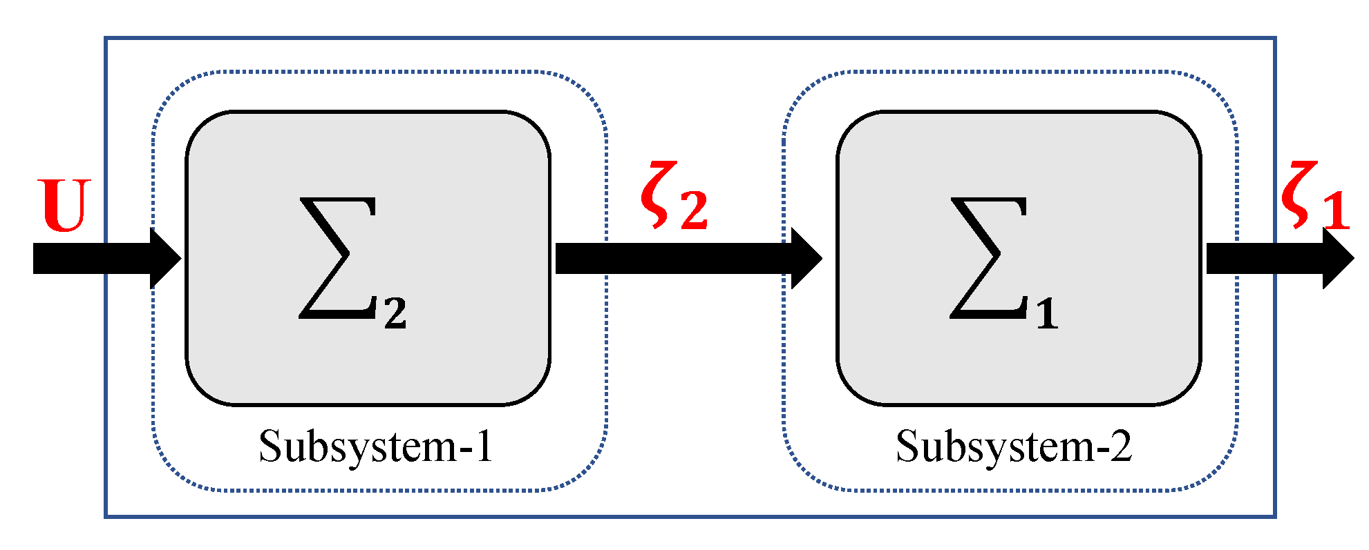
To tackle these challenges, control strategies grounded in the cascaded theory have been introduced, as discussed in [20,21]. In [20], the authors have designed a controller using sliding mode control (SMC) to increase the speed of the convergence time. To develop a robust cascaded system for the NWMR, ref. [21] introduces a continuous SMC along with two nonlinear disturbance observers. Therefore, in this work, we adopt the cascade theory for the multiple NWMRs’ system control design. The cascade control theory is particularly effective for hierarchical and modular multi-robot control problems such as leader–follower formations. It enables decomposition of the overall system into subsystems—one for the leader’s trajectory tracking and another for the follower’s formation maintenance. This modularity simplifies both the controller design and stability analysis. The control design is divided into two components: one focuses on enabling the leader robot to track the reference path, while the other ensures that the follower robots maintain the target formation and follow the leader. Another major advantage of the cascade approach is that it supports scalability and robustness. It allows the follower subsystem to estimate leader states using only local communication, avoiding reliance on global information, which is often assumed in consensus-based or centralized approaches. Additionally, the use of the Lyapunov theory within the cascade framework facilitates rigorous stability guarantees for each subsystem and their interconnection. For these two sections, the global control law is used to stabilize one subsystem. Moreover, another subsystem is stabilized by the SMC designed for the leader. In order to keep the formation pattern, PD control is also employed for follower robots to relax the severe limits on the intended velocities.

Building upon the above investigations, this work focuses on designing a control scheme for leader–follower formation of multiple NWMRs using a distributed estimator-based cascade control framework. In this approach, each follower robot employs a distributed estimator to reconstruct the leader’s state information. The main contributions of this study are summarized as follows:

• A distributed estimator-based leader–follower formation control scheme is proposed for a swarm of multiple NWMRs.
• A sliding mode control (SMC) law is developed for the leader robot based on the cascade theory.
• A distributed estimator–controller is designed for each follower to estimate the leader’s position, orientation, linear velocity, and angular velocity.
• Lyapunov stability and cascade system theory are used to guarantee closed-loop error convergence. Theoretical results are validated through comprehensive simulation experiments.

2. Preliminaries and Problem Statement

2.1. Preliminaries

2.1.1. Notations

The N-dimensional zero column vector and $N\times N$ matrix are denoted as $0_N$ and $I_N$, respectively. For the simple vector $A={[a_1,a_2,\dots a_N]}^T\in {\mathbb{R}}_N$, its Euclidean norms can be denoted as ${\parallel A\parallel }_2=\sqrt{A^{T}A}$. Further, the ${\lambda }_m$ denotes the eigenvalues of given symmetric matrix $P\in {\mathbb{R}}_{N\times N}$, defined as ${\lambda }_{min}\left(P\right)={\lambda }_1\left(P\right)\le {\lambda }_2\left(P\right)\le \cdots \le {\lambda }_N\left(P\right)={\lambda }_{max}\left(P\right)$.

2.1.2. Definitions

Definition 1

([22]). A continuous function $a:[0,\alpha )\to [0,\infty )$ is defined as a class-$\mathcal{K}$ function when a is strictly increasing and $a\left(0\right)=0$.

A continuous function $b:[0,\alpha )\times [0,\alpha )\to [0,\infty )$ is defined as one of class-$\mathcal{KL}$ function, then the following two states should be satisfied.

→

when fixed for all q, $\beta (p,q)$ is a class $\mathcal{K}$ function with respect to p and

→

when fixed for all p, $\beta (p,q)$ is decreasing with respect to q and $\beta (p,q)\to 0$ and $q\to \infty$.

The following system is considered as

$$\dot{\zeta }=\mathrm{\Pi }(t,\zeta ),\mathrm{\Pi }(t,0)=0,\forall t\ge 0,$$

(1)

where $\mathrm{\Pi }:{\mathbb{R}}_{\ge 0}\times {\mathbb{R}}_N\to {\mathbb{R}}_N$ is locally Lipschitz in ζ and sectionally continuous in time t.

Definition 2

([22]). The system (1) is globally uniformly asymptotically stable (GUAS); if a class $\mathcal{KL}$ function exists, then the function $b(·,·)$ is such that, for all initial states $\zeta \left(t_0\right)$,

$${\parallel \zeta \left(t\right)\parallel }_2\le b(\parallel \zeta \left(t_0\right){\parallel }_2,t-t_0),\forall t\ge t_0\ge 0.$$

(2)

2.1.3. Cascade System

In the nonlinear systems, a separate principle is applied to control two coupled systems without affecting the general form of the systems. Based on this working principle, we introduced the cascade system in our proposed work. The cascade system [20,23] is applied into the complex nonlinear system to analyze by simply dividing it into subsystems. Figure 1 shows the cascade system of two sub-problems, such that the system stability problems are analyzed by considering that both subsystems separately are stable and they conserve that property when interconnected.

To assess the stability of the final closed-loop system, the systems outlined below must be implemented. Therefore, these systems are introduced as follows:

$$\begin{array}{cc}\hfill \dot{{\zeta }_1}& ={\mathrm{\Pi }}_1(t,{\zeta }_1)+{\mathrm{\Psi }}_1(t,{\zeta }_1,{\zeta }_2)\hfill \end{array}$$

(3a)

$$\begin{array}{cc}\hfill \dot{{\zeta }_2}& ={\mathrm{\Pi }}_2(t,{\zeta }_2)\hfill \end{array}$$

(3b)

where ${\zeta }_1\in {\mathbb{R}}_2$, ${\zeta }_2\in \mathbb{R}$, $\zeta ={[{\zeta }_1^T,{\zeta }_2^T]}^T$, and the functions ${\mathrm{\Pi }}_1(·,·)$, ${\mathrm{\Pi }}_2(·,·)$, and ${\mathrm{\Psi }}_1(·,·,·)$ are continuous in their arguments, locally Lipschitz in $\zeta$, and uniform in t, and ${\mathrm{\Pi }}_1(·,·)$ is continuously differentiable in both arguments.

Moreover, we assume ${\zeta }_2=0$, and Equation (3a) follows as follows:

$$\begin{array}{c}\hfill \dot{{\zeta }_1}={\mathrm{\Pi }}_1(t,{\zeta }_1).\end{array}$$

(4)

Therefore, Equation (3a) can be considered a subsystem

$$\begin{array}{c}\hfill {\mathrm{\Sigma }}_1:\dot{{\zeta }_1}={\mathrm{\Pi }}_1(t,{\zeta }_1)\end{array}$$

(5)

which is perturbed by the subsystems listed below:

$$\begin{array}{c}\hfill {\mathrm{\Sigma }}_2:\dot{{\zeta }_2}={\mathrm{\Pi }}_2(t,{\zeta }_2).\end{array}$$

(6)

Moreover, the cascade-interconnected states are denoted as ${\mathrm{\Psi }}_1(t,{\zeta }_1,{\zeta }_2)$.

Lemma 1.

Let us consider the cascade system (3a) and (3b), if the following three conditions [C1]–[C3] hold, then the systems (3a) and (3b) are GUAS:

[C1]: Assume that the subsystem ${\mathrm{\Sigma }}_1:\dot{{\zeta }_1}={\mathrm{\Pi }}_1(t,{\zeta }_1)$ is GUAS and that there exists an auxiliary positive definite Lyapunov function candidate $V(t,{\zeta }_1):{\mathbb{R}}_{\ge 0}\times {\mathbb{R}}_n\to {\mathbb{R}}_{\ge 0}$ such that

$$W_1\left({\zeta }_1\right)\le V(t,{\zeta }_1)\le W_2\left({\zeta }_1\right)$$

(7)

$${\displaystyle \frac{\partial V(t,{\zeta }_1)}{\partial t}}+{\displaystyle \frac{\partial V(t,{\zeta }_1)}{\partial {\zeta }_1}}{\mathrm{\Pi }}_1(t,{\zeta }_1)\le -W\left({\zeta }_1\right)$$

(8)

where $W_1\left({\zeta }_1\right)$ and $W_2\left({\zeta }_1\right)$ are two class ${\mathcal{K}}_{\infty }$ functions, $W\left({\zeta }_1\right)$ is a positive semi-definite function. Further simplifying Equation (8), we have

$$\parallel {\displaystyle \frac{\partial V(t,{\zeta }_1)}{\partial {\zeta }_1}}\parallel \parallel {\zeta }_1\parallel \le c_{1}V(t,{\zeta }_1)\forall \parallel {\zeta }_1\parallel \ge \kappa$$

(9)

where $c_1>0$, $\kappa >0$, and $c_2>0$ are some constants. Furthermore, ${\displaystyle \frac{\partial V(t,{\zeta }_1)}{\partial {\zeta }_1}}(t,\zeta )$ is bounded uniformly in t for all $\parallel \zeta \parallel \le \kappa$. In other words, there exist constants $c_2>0$ and $t\ge t_0\ge 0$ such that

$$\parallel {\displaystyle \frac{\partial V(t,{\zeta }_1)}{\partial {\zeta }_1}}\parallel \le c_2\forall \parallel {\zeta }_1\parallel \le \kappa$$

(10)

[C2]: The function ${\mathrm{\Psi }}_1(t,{\zeta }_1,{\zeta }_2)$ satisfies that for all ${\zeta }_1\in {\mathbb{R}}_{N1}$ and all ${\zeta }_2\in {\mathbb{R}}_N$, for all $t\ge t_0\ge 0$, there exist

$$\parallel g(t,{\zeta }_1,{\zeta }_2)\parallel \le \parallel {\zeta }_2\parallel ({\mathrm{\Phi }}_1(\parallel {\zeta }_2\parallel )+\parallel {\zeta }_1\parallel {\mathrm{\Phi }}_2(\parallel {\zeta }_2\parallel \left)\right)$$

(11)

where ${\mathrm{\Phi }}_1,{\mathrm{\Phi }}_2:{\mathbb{R}}_{\ge 0}\mapsto {\mathbb{R}}_{\ge 0}$ are continuous functions.

[C3]: Assume that the subsystem ${\mathrm{\Sigma }}_2:\dot{{\zeta }_2}={\mathrm{\Pi }}_2(t,{\zeta }_2)$ is GUAS and for all $t\ge t_0\ge 0$, there exists a class-$\mathcal{K}$ function $f(.)$ satisfying

$${\int }_{t_0}^{\infty }\parallel {\zeta }_2(t,t_0,\mathrm{\Pi }\left(t_0\right))\parallel dt\le f(\parallel {\zeta }_2\left(t_0\right)\parallel )$$

(12)

2.1.4. Graph Theory

In this proposed work, the communication topology of the multiple robot formations is represented by graph theory. We consider the leader–follower formation of NWMRs with one leader ($R_0$) and N followers ($R_N$). The interaction among the robots can be represented by a directed graph $\mathcal{G}=(\mathcal{V},\mathcal{E},\mathcal{A})$, where $\mathcal{V}\in \{R_0,R_1,R_2,\dots ,R_N\}$ represents the set of robot nodes, $\mathcal{E}\subseteq \mathcal{V}\times \mathcal{V}$ is an edge set with element $(i,j)$ that describes the communication between the $R_i^{th}$ robot to the $R_j^{th}$ robot. Moreover, $\mathcal{A}\in {\mathbb{R}}_{N\times N}$ represents the adjacency matrix with nonnegative elements. In the directed graph, the state of robot $R_i$ is available to robot $R_j$, then the edges can be denoted as $(R_i,R_j)\in \mathcal{E}$, which means that node $R_i$ can access node $R_j$. The weight adjacency matrix is defined as $\mathcal{A}={\left[a_{ij}\right]}_{N\times N}$, and the element $a_{ij}$ associated with the arc of the digraph is positive; that is, $a_{ij}>0⟺(R_i,R_j)\in \mathcal{E}$. The set of neighbors for robot i is ${\mathcal{N}}_i=\{j\in \mathcal{V}|(j,i)\in \mathcal{E}\left(\mathcal{G}\right)\}$. Furthermore, the adjacency matrix is defined as follows:

$$a_{ij}=\left\{\begin{array}{c}\begin{array}{cc}1,& \mathrm{for}(R_j,R_i)\in \mathcal{E},\\ 0,& \mathrm{otherwise}.\end{array}\hfill \end{array}\right.$$

(13)

We assume that $a_{ii}=0$ for all $R_i$. Define $d_i={\sum }_{j=1}^N{a}_{ij}$ as the indegree of robot $R_i$, and $D\in {\mathbb{R}}_{N\times N}$ is a diagonal matrix which consists of $D=\mathrm{diag}\{d_0,d_1,d_2,\cdots d_N\}\in {\mathbb{R}}_{N\times N}$. Then, the Laplacian matrix is defined as $L=D-A$, where $L=\left[l_{ij}\right]\in {\mathbb{R}}_{N\times N}$, where $l_{ij}$ is defined as follows:

$$l_{ij}=\left\{\begin{array}{c}\begin{array}{cc}-a_{ij},& \mathrm{for}(R_j\ne R_i),\\ {\sum }_{j=1,j\ne i}^N{a}_{ij},& \mathrm{for}(R_j=R_i).\end{array}\hfill \end{array}\right.$$

(14)

Next, we introduce the reference $R_r$ to the leader NWMR for leading the trajectory of the whole systems. Moreover, the proposed communication topology between the multiple NWMRs systems can be represented by the leader adjacency matrix $a={[a_{10},a_{20},\cdots ,a_{N0}]}^T$ and the adjacency weight is defined as

$$a_{i0}=\left\{\begin{array}{c}\begin{array}{cc}1,& \mathrm{If}\mathrm{the}{R}_0\mathrm{is}\mathrm{neighbor}\mathrm{of}{R}_N,\\ 0,& \mathrm{otherwise}.\end{array}\hfill \end{array}\right.$$

(15)

The matrix $H\in {\mathbb{R}}_{N\times N}$ can be described by

$$H=L+\mathrm{diag}\left(a\right).$$

(16)

The matrix H has been climbed by following based on the result [24].

Lemma 2.

Matrix H is symmetric positive definite if and only if the directed graph $\mathcal{G}$ is connected, and the leader is a neighbor of at least one follower, i.e., at least one $a_{i0}>0$.

To further strengthen robustness, assume that the communication graph contains a directed spanning tree rooted at the leader. This structure guarantees that information can flow indirectly from the leader to all followers, even when direct communication links are absent. Each follower robot employs a PD-based distributed estimator that uses only local neighbor information, without requiring global or centralized communication—to estimate the leader’s state. This design ensures that the estimator remains functional under communication constraints, such as packet loss, limited bandwidth, or time-varying topologies, to validate the resilience of this estimator framework under communication delays and topology changes, as described in the sensitivity analysis section of the manuscript. These evaluations confirm that the proposed method reliably maintains estimation accuracy and system stability under practical communication limitations.

2.1.5. Kinematic Model of the Mobile Robot

The kinematic model of the NWMR system is demonstrated in Figure 2. The NWMR is fully described by a 3D vector of generalized coordinates $q={[x,y,\theta ]}^T$, where q is formed by the center point of the two driving wheels of the robot coordinates $(x,y)$ and the orientation angle $\theta$.

The kinematic model of the NWMR in Cartesian frame coordinates is given by

$$\dot{q}=\left[\begin{array}{c}\dot{x}\\ \dot{y}\\ \dot{\theta }\end{array}\right]=\left[\begin{array}{cc}cos\theta & 0\\ sin\theta & 0\\ 0& 1\end{array}\right]\left[\begin{array}{c}v\\ \omega \end{array}\right].$$

(17)

Assumption 1.

The directed graph $\mathcal{G}$ among the multi-robot system contains the number of robots $R_{\mathcal{N}}$ (where $R_{\mathcal{N}}$ contains a leader robot $R_0$ and multiple followers $R_N$). The directed graph contains the directed spanning tree with the leader robot $R_0$ as the root node has direct access to the desired trajectory.

The primary goal of our method is to develop the control law for multiple NWMR systems in order to hold the desired shape of the formation with respect to its position and orientation. Based on the directed graph $\mathcal{G}$ with nonholonomic properties of given NWMR model, the desired formation pattern of the multiple follower robots is specified by the certain distance vectors ${\Delta }_i=[{\Delta }_{ix}$ ${\Delta }_{iy}{]}^T$ from the leader robots. The leader–follower formation approach presented by the Cartesian coordinates is shown in Figure 3.

In the development process of designing the tracking controller, initially, the control law $v_0$ and ${\omega }_0$ are designed for the leader robot $R_0$ based on the reference, such that the following objective is achieved.

$$\begin{array}{cc}\hfill & \underset{t\to \infty }{lim}(x_0\left(t\right)-x_r\left(t\right))=0,\hfill \\ \hfill & \underset{t\to \infty }{lim}(y_0\left(t\right)-y_r\left(t\right))=0,\hfill \\ \hfill & \underset{t\to \infty }{lim}({\theta }_0\left(t\right)-{\theta }_r\left(t\right))=0.\hfill \end{array}$$

(18)

Furthermore, based on the distributed controller, the control laws are formulated for the multiple follower robots $R_N$ to maintain the desired formation pattern such that the following objective can be achieved.

$$\begin{array}{cc}\hfill & \underset{t\to \infty }{lim}(x_i\left(t\right)-x_r\left(t\right))={\Delta }_{xi},\hfill \\ \hfill & \underset{t\to \infty }{lim}(y_i\left(t\right)-y_r\left(t\right))={\Delta }_{yi},\hfill \\ \hfill & \underset{t\to \infty }{lim}({\theta }_i\left(t\right)-{\theta }_r\left(t\right))=0,\hfill \end{array}$$

(19)

where $[{\Delta }_{xi}$ ${\Delta }_{yi}{]}^T$ is the desired relative position between $R_0$ and $R_i$.

Remark 1.

From the above discussions, based on the virtual robot $R_r$ path, Equation (18) guarantees that the leader robot $R_0$ will eventually match the virtual trajectory. In addition to this, Equation (19) guarantees that all of the following robots will eventually converge on the correct geometric structure. In other words, if conditions (18) and (19) are met, the intended formation goal can be achieved.

2.2. Problem Statement

In a problem of leader–follower formation, the follower robots should preserve the desired geometric pattern when following the leader trajectory. Consider a group of $N+1$ two wheeled NWMRs robot $R_i$, ($i=0,1,\dots ,N$) where $R_0$ and $(R_1\cdots R_N)$ represent the leader and follower robots, respectively. The kinematic model of each robot can be expressed as

$$\begin{array}{cc}\hfill \dot{x_i}& =v_{i}cos{\theta }_i,\hfill \\ \hfill \dot{y_i}& =v_{i}sin{\theta }_i,\hfill \\ \hfill \dot{{\theta }_i}& ={\omega }_i,\hfill \end{array}$$

(20)

where $(x_i,y_i)\in {\mathbb{R}}_2$ denotes the position of $\left(R_i\right)$, and ${\theta }_i\in \mathbb{R}$ is the orientation of $R_i$. Moreover, the control inputs $v_i$ and ${\omega }_i$ are the linear and angular velocity of the robots $R_i$.

In the task of trajectory tracking, the desired trajectory for the leader robot $R_0$ is developed by the robot $R_r$. The states of the reference robot $R_r$ are described by

$$\begin{array}{cc}\hfill {\dot{x}}_r& =v_{r}cos{\theta }_r,\hfill \\ \hfill {\dot{y}}_r& =v_{r}sin{\theta }_r,\hfill \\ \hfill {\dot{\theta }}_r& ={\omega }_r,\hfill \end{array}$$

(21)

where $x_r,y_r$ represent the location and ${\theta }_r$ represent the direction angle of the reference robot $R_r$. Moreover, $v_r$ and ${\omega }_r$ denote the reference robot’s linear and angular velocities, respectively.

In the proposed leader–follower framework, follower robots do not rely on direct communication with the leader robot $R_0$. Instead, each follower employs a PD-based distributed estimator to infer the leader’s position, velocity, and orientation using only information from local neighbors defined by the graph topology. This decentralized estimation strategy reduces communication overhead and improves robustness to delays, packet loss, and topological changes. These communication-aware estimation features are validated through a sensitivity analysis and discussed in Section 2.1.4.

3. Formation Control Law Design and Stability Analysis

This section explains the proposed leader–follower formation method in three parts. First, we design a controller for the leader robot $R_0$ which ensures the tracking errors converge to zero. Secondly, we present a novel distributed estimator to enable the followers to estimate the leader’s state information. Thirdly, we design tracking controllers for the follower robot $R_N$ using the distributed estimator, ensuring that the desired geometric formation is achieved. The proposed formation control design and the control system block diagram of the proposed leader–follower framework for NMRs are shown in Figure 4 and Figure 5.

3.1. Leader Control Design for Tracking

In this subsection, we design a trajectory tracking controller for the leader robot $R_0$, which helps to track the virtual robot $R_r$’s trajectory. To develop the trajectory tracking controller for $R_0$, we introduce the error state vector that represents the difference between the leader and the reference robot, as shown in Figure 3. The error state vectors $q_{e0}={[x_{e0},y_{e0},{\theta }_{e0}]}^T$ are given by

$$e_{x0}=x_r-x_0,$$

(22a)

$$e_{y0}=y_r-y_0,$$

(22b)

$$e_{\theta 0}={\theta }_r-{\theta }_0.$$

(22c)

The following transformation matrix is defined as

$$\left[\begin{array}{c}{x}_{e0}\\ y_{e0}\\ {\theta }_{e0}\end{array}\right]=\left[\begin{array}{ccc}cos{\theta }_0& sin{\theta }_0& 0\\ -sin{\theta }_0& cos{\theta }_0& 0\\ 0& 0& 1\end{array}\right]\left[\begin{array}{c}{e}_{x0}\\ e_{y0}\\ e_{\theta 0}\end{array}\right]$$

(23)

By taking the derivative of Equation (23), one can obtain the following error dynamics:

$${\dot{x}}_{e0}={\omega }_0{y}_{e0}-v_0+v_{r}cos{\theta }_{e0},$$

(24a)

$${\dot{y}}_{e0}=-{\omega }_0{x}_{e0}+v_{r}sin{\theta }_{e0},$$

(24b)

$${\dot{\theta }}_{e0}={\omega }_r-{\omega }_0.$$

(24c)

3.1.1. Design of Angular Control Strategy

Following the cascade system approach, the error tracking Equation (24c) resembles the first-order subsystem (6). Hence, the angular control strategy for the leader is formulated as follows:

$$\begin{array}{c}\hfill {\omega }_0={\omega }_r+{\theta }_{e0}+k_3{\theta }_{e0}.\end{array}$$

(25)

Then, the angular control velocity is formulated as follows:

$$\begin{array}{c}\hfill {\dot{\theta }}_{e0}=-{\theta }_{e0}-k_3{\theta }_{e0}.\end{array}$$

(26)

Theorem 1.

Consider system (24c), there is a control law (25) in such a way that the system satisfies the GUAS.

Proof. 

According to the designed angular velocity ${\theta }_{e0}+k_3{\theta }_{e0}=0$, we obtain the state ${\theta }_{e0}=0$. In order to examine systems (24c) and (25)’s stability, We express the Lyapunov function as follows:

$$\begin{array}{c}\hfill V={\displaystyle \frac{1}{2}}{\theta }_{e0}^2.\end{array}$$

(27)

Taking the derivative of (27) and using (26), we have

$$\begin{array}{cc}\hfill \dot{V}& ={\theta }_{e0}{\dot{\theta }}_{e0}={\theta }_{e0}(-{\theta }_{e0}-k_3{\theta }_{e0})=-{\theta }_{e0}^2-k_3{\theta }_{e0}^2,\hfill \\ \hfill \dot{V}& \le 0(\dot{V}=0\mathrm{if}\mathrm{and}\mathrm{only}\mathrm{if}{\theta }_{e0}=0).\hfill \end{array}$$

(28)

Hence, the closed-loop system (24c) is GUAS. □

3.1.2. Forward Velocity Control Law Design

The angular control (25), which drives the angular error to zero, plays a crucial role. Consequently, the error tracking system (24) can be simplified as follows:

$${\dot{x}}_{e0}={\omega }_r{y}_{e0}-v_0+v_r,$$

(29a)

$${\dot{y}}_{e0}=-{\omega }_r{x}_{e0}.$$

(29b)

Moreover, Equation (29) can be transformed into following form:

$$\left[\begin{array}{c}{\dot{x}}_{e0}\\ {\dot{y}}_{e0}\end{array}\right]=\left[\begin{array}{cc}0& {\omega }_r\\ -{\omega }_r& 0\end{array}\right]\left[\begin{array}{c}{x}_{e0}\\ y_{e0}\end{array}\right]+\left[\begin{array}{c}1\\ 0\end{array}\right]\left[\begin{array}{c}{v}_r-v_0\end{array}\right].$$

(30)

Define $X\left(t\right)=\left[\begin{array}{c}{\dot{x}}_{e0}\\ {\dot{y}}_{e0}\end{array}\right]$, $A_1\left(t\right)=\left[\begin{array}{cc}0& {\omega }_r\\ -{\omega }_r& 0\end{array}\right]$, $B_1\left(t\right)=\left[\begin{array}{c}1\\ 0\end{array}\right]$ and $U\left(t\right)=\left[\begin{array}{c}{v}_r-v_0\end{array}\right]$.

Therefore, we define the following system:

$$X\left(t\right)=A_1\left(t\right)X\left(t\right)+B_1\left(t\right)U\left(t\right).$$

(31)

Furthermore, the system’s stability (31) must be analyzed. Applying the controllability criterion, we obtain the following:

$$M_1\left(t\right)=B_1\left(t\right)=\left[\begin{array}{c}1\\ 0\end{array}\right]$$

$$M_2\left(t\right)=-A_1\left(t\right)M_1\left(t\right)+{\displaystyle \frac{d}{dt}}{M}_1\left(t\right)=\left[\begin{array}{c}0\\ w_r\end{array}\right]$$

Furthermore, we do as follows:

$$\begin{array}{cc}\hfill \mathrm{Rank}[M_1\left(t\right):M_2\left(t\right)]& =\mathrm{Rank}\left[A_1\left(t\right)\right],\hfill \\ \hfill \mathrm{Rank}\left[\begin{array}{cc}1& 0\\ 0& {\omega }_r\end{array}\right]& =\mathrm{Rank}\left[\begin{array}{cc}0& {\omega }_r\\ -{\omega }_r& 0\end{array}\right]=2\hfill \end{array}$$

(32)

where ${\omega }_r\ne 0$. This means that system (31) is said to be controllable.

Based on the cascade system theory, when ${\omega }_r\ne 0$, we can consider that (29) is the subsystem ${\mathrm{\Sigma }}_1$. Further, we consider the state in Equation (29b) and we design the state $x_{e0}$ as a feedback so that the state $y_{e0}$ is stabilized to zero.

Theorem 2.

Consider the system (29b). It should be noted that $w_r\ne 0$, and $k_0$ is a positive constant ($k_0>0$). Under these conditions, there exists $x_{e0}=k_0{y}_{e0}\mathit{sgn}\left(w_r\right)$, where $\mathit{sgn}\left(w_r\right)$ denotes the sign function, ensuring that system (29b) is globally uniformly stable.

Proof. 

The state reaches the equilibrium point of (29b) with $-w_r{x}_{e0}=0$, when $x_{e0}=0$. Hence, the (29b) subsystem has an equilibrium point. Using the Lyapunov theory, we examine the stability of (29b) as follows:

$$\begin{array}{cc}\hfill V\left(y_{e0}\right)& ={\displaystyle \frac{1}{2}}{y}_{e0}^2,\hfill \\ \hfill \dot{V}\left(y_{e0}\right)& =y_{e0}{\dot{y}}_{e0}=y_{e0}(-w_r{x}_e)=-y_{e0}\left(k_0{y}_{e0}sgn\left(w_r\right)\right),\hfill \\ \hfill & =-k_0{y}_{e0}^2{w}_{r}sgn\left(w_r\right)\Rightarrow \dot{V}\left(y_{e0}\right)\le 0.\hfill \end{array}$$

□

We notice that $sgn\left(w_r\right)>0$ when $w_r>0$ and $sgn\left(w_r\right)<0$ when $w_r<0$ means $w_{r}sgn\left(w_r\right)>0$. Also, $\dot{V}\left(y_{e0}\right)\le 0$$(\dot{V}\left(y_{e0}\right)=0$ if and only if $y_{e0}=0)$. Hence, system (29b) is GUAS.

Moreover, the sliding manifold is defined by

$$S=x_{e0}-k_0{y}_{e0}sgn\left(w_r\right).$$

(33)

By using $x_{e0}=k_0{y}_{e0}sgn\left(w_r\right)$, we have

$$S=x_{e0}-k_0{y}_{e0}sgn\left(w_r\right)=0.$$

(34)

To verify the stability of the sliding surface S, we require that $\dot{S}S<0$. The derivative $\dot{S}$ is given by

$$\dot{S}=-S-\alpha S$$

(35)

where $\alpha \ge 0$. From Equation (29) to Equation (35), the sliding mode controller is designed as follows:

$$\begin{array}{cc}\hfill \dot{S}& =-S-\alpha S={\dot{x}}_{e0}-k_0{\dot{y}}_{e0}sgn\left(w_r\right),\hfill \\ \hfill & =w_r{y}_{e0}-v+v_r-k_0(-w_r{x}_{e0})sgn\left(w_r\right).\hfill \end{array}$$

(36)

From Equation (36), we obtain the linear control for the leader as follows:

$$\begin{array}{c}\hfill v=v_r+w_r{y}_{e0}+k_0{w}_r{x}_{e0}sgn\left(w_r\right)+S+\alpha S.\end{array}$$

(37)

We can establish the velocity control law of the leader robot using sliding mode control, which ensures GUAS of the closed-loop subsystems (29a) and (29b).

Remark 2.

In this article, sliding manifold is chosen as in (33) along with the reaching law (35), which ensures that the state $x_{e0}$ will converge to $k_0{y}_{e0}sgn\left(w_r\right)$. Based on Theorem 3, with the change of convergence time, we can understand that the state $y_{e0}$ converges to zero. From this, we clearly conclude that the state $x_{e0}=0$, when the state $y_{e0}=0$.

Remark 3.

From the existing literature [25,26], the desired angular velocity $w_r$ should satisfy $0<w_r^{min}\le \parallel w_r\parallel \le w_r^{max}$, where $w_r^{min}$ and $w_r^{max}$ are constants. Different from the existing works, in this study, the desired angular velocity $w_r$ has to satisfy $w_r\ne 0$ only. Therefore, the proposed control laws relax the conditions about the velocities which have been reported in the literature.

Additionally, we must examine the stability of the error dynamics (24) using the leader’s control laws (25) and (37). Since the sliding surface S converges to zero, we can obtain $x_{e0}=k_0{y}_{e0}\mathrm{sgn}\left(w_r\right)$, and (37) will be modified as follows:

$$\begin{array}{c}\hfill v=v_r+w_r{y}_{e0}+k_0{w}_r{x}_{e0}sgn\left(w_r\right)\end{array}$$

(38)

Substituting (25) and (38) into error system (24), we have

$$\left[\begin{array}{c}{x}_{e0}\\ y_{e0}\end{array}\right]=\left[\begin{array}{c}{k}_0{w}_r{x}_{e0}sgn\left(w_r\right)\\ x_{e0}{w}_r\end{array}\right]+\left[\begin{array}{c}{y}_{e0}\mathcal{F}\left({\theta }_{e0}\right)+v_r(cos({\theta }_{e0}-1)\\ v_{r}sin{\theta }_{e0}-x_{e0}\mathcal{F}\left({\theta }_{e0}\right)\end{array}\right]$$

(39)

$${\dot{\theta }}_{e0}=-\mathcal{F}\left({\theta }_{e0}\right)$$

(40)

where $\mathcal{F}\left({\theta }_{e0}\right)={\theta }_{e0}+{\alpha }_1{\theta }_{e0}$. Using the cascade theory as in Section 2.1.3, we obtain,

$$\begin{array}{cc}\hfill {\mathrm{\Pi }}_1(t,{\zeta }_1)& =\left[\begin{array}{c}{k}_0{w}_r{x}_{e0}sgn\left(w_r\right)\\ x_{e0}{w}_r\end{array}\right],{\mathrm{\Psi }}_1(t,{\zeta }_1,{\zeta }_2)=\left[\begin{array}{c}{y}_{e0}\mathcal{F}\left({\theta }_{e0}\right)+v_r(cos({\theta }_{e0}-1)\\ v_{r}sin{\theta }_{e0}-x_{e0}\mathcal{F}\left({\theta }_{e0}\right)\end{array}\right]\hfill \\ \hfill {\mathrm{\Pi }}_2(t,{\zeta }_2)& =-\mathcal{F}\left({\theta }_{e0}\right)\hfill \end{array}$$

consider the state transformation defined as $\dot{{\zeta }_1}={\left[x_{e0}{y}_{e0}\right]}^T,\dot{{\zeta }_2}={\theta }_{e0}$. The derivatives of $\dot{{\zeta }_1}$ and $\dot{{\zeta }_2}$ are $\dot{{\zeta }_1}={\mathrm{\Pi }}_1(t,{\zeta }_1)+{\mathrm{\Psi }}_1(t,{\zeta }_1,{\zeta }_2)$ and $\dot{{\zeta }_2}={\mathrm{\Pi }}_2(t,{\zeta }_2)$, which is similar to system (3). By utilizing the cascade system theory, the following conditions will be established.

[1]: Consider the subsystem ${\dot{\zeta }}_1={\mathrm{\Pi }}_1(t,{\zeta }_1)$. We select the Lyapunov function as follows:

$$\begin{array}{c}\hfill V_1={\displaystyle \frac{1}{2}}{x}_{e0}+{\displaystyle \frac{1}{2}}{y}_{e0}.\end{array}$$

(41)

Taking the derivative of Equation (41) along with the subsystems (29), we have

$$\begin{array}{cc}\hfill \dot{V_1}& =x_{e0}{\dot{x}}_{e0}+y_{e0}{\dot{y}}_{e0}=x_{e0}(w_r{y}_{e0}-v+v_r)+y_{e0}(-w_r{x}_{e0}),\hfill \\ \hfill & =x_{e0}(-k_0{w}_r{x}_{e0}sgn\left(w_r\right))+y_{e0}(-w_r-k_0{y}_{e0}sgn\left(w_r\right)),\hfill \\ \hfill & =-k_0{w}_r{x}_{e0}^{2}sgn\left(w_r\right)-k_0{w}_r{y}_{e0}^{2}sgn\left(w_r\right).\hfill \end{array}$$

Note that $w_{r}sgn\left(w_r\right)>0$ and $k_0>0$; we obtain $\dot{V_1}\le 0$ ($\dot{V_1}=0$, if $x_{e0}=y_{e0}=0$), which means that ${\dot{\zeta }}_1={\mathrm{\Pi }}_1(t,{\zeta }_1)$ satisfies condition [C1] of Section 2.1.3. Hence, the subsystem ${\mathrm{\Pi }}_1(t,{\zeta }_1)$ is GUAS.

[2]: Consider the subsystem ${\dot{\zeta }}_2={\mathrm{\Pi }}_2(t,{\zeta }_2)$, the stability analysis is verified by the proof of Theorem 1 in which the subsystem ${\mathrm{\Pi }}_2(t,{\zeta }_2)$ is proven as GUAS.

[3]: Consider the subsystem ${\mathrm{\Psi }}_1(t,{\zeta }_1,{\zeta }_2)$, we can select the Lyapunov function as follows:

$$\begin{array}{c}\hfill V_2={\displaystyle \frac{1}{2}}{x}_{e0}+{\displaystyle \frac{1}{2}}{y}_{e0}.\end{array}$$

(42)

Taking the derivative of (42) along with the system (39), we obtain

$$\begin{array}{cc}\hfill \dot{V_2}=& x_{e0}{\dot{x}}_{e0}+y_{e0}{\dot{y}}_{e0},\hfill \\ \hfill =& x_{e0}[-k_0{w}_r{x}_{e0}sgn\left(w_r\right)+y_{e0}\mathcal{F}\left({\theta }_{e0}\right)+v_r(cos({\theta }_{e0}-1)]\hfill \\ & +y_{e0}[-x_{e0}{w}_r+v_{r}sin{\theta }_{e0}-x_{e0}\mathcal{F}\left({\theta }_{e0}\right)],\hfill \\ \hfill =& -k_0{w}_r{x}_{e0}^{2}sgn\left(w_r\right)-k_0{w}_r{x}_{e0}^{2}sgn\left(w_r\right)+v_r{x}_{e0}(cos{\theta }_{e0}-1)+v_r{y}_{e0}sin{\theta }_{e0}],\hfill \\ \hfill \le & v_r[x_{e0}(cos{\theta }_{e0}-1)+y_{e0}sin{\theta }_{e0}]\le 2v_r^{max}\parallel {\mathrm{\Pi }}_1\parallel .\hfill \end{array}$$

Therefore, ${\mathrm{\Psi }}_1(t,{\zeta }_1,{\zeta }_2)$ satisfies [C3] as in Section 2.1.3. Hence, it shows that the subsystem ${\mathrm{\Psi }}_1(t,{\zeta }_1,{\zeta }_2)$ is GUAS.

3.2. Distributed Formation Controller Design for Multiple Followers

In this subsection, we have to design the controllers for the follower robots $R_N$ (where $N=1,2,\cdots ,N$), which helps to follow the leader $R_0$ path with the desired geometric pattern. Indeed, the leader robot’s information includes the positions $(x_0,y_0)$, orientations ${\theta }_0$, linear velocity $v_0$, and angular velocity ${\omega }_0$ that is not accessible for some follower robots for a large group. To address this issue, inspired by [27], we propose a distributed estimator for each follower to estimate the leader’s information. The designed distributed estimator for N followers is given as follows:

$${\dot{\widehat{x}}}_i={\widehat{v}}_{i}cos{\widehat{\theta }}_i+{\gamma }_i(x_0-{\widehat{x}}_i)+\sum _{j\in N_i}({\widehat{x}}_j-{\widehat{x}}_i),$$

(43)

$${\dot{\widehat{y}}}_i={\widehat{v}}_{i}sin{\widehat{\theta }}_i+{\gamma }_i(y_0-{\widehat{y}}_i)+\sum _{j\in N_i}({\widehat{y}}_j-{\widehat{y}}_i),$$

(44)

$${\dot{\widehat{\theta }}}_i={\widehat{\omega }}_i+{\gamma }_i({\omega }_0-{\widehat{\omega }}_i)+\sum _{j\in N_i}({\widehat{\omega }}_j-{\widehat{\omega }}_i),$$

(45)

$${\dot{\widehat{v}}}_i={\mu }_1\left({\gamma }_i(v_0-{\widehat{v}}_i)+\sum _{j\in N_i}({\widehat{v}}_j-{\widehat{v}}_i)\right)+{\mu }_2\left({\gamma }_i(v_0-{\widehat{v}}_i)+\sum _{j\in N_i}({\widehat{v}}_j-{\widehat{v}}_i)\right),$$

(46)

$${\dot{\widehat{\omega }}}_i={\mu }_3\left({\gamma }_i({\omega }_0-{\widehat{\omega }}_i)+\sum _{j\in N_i}({\widehat{\omega }}_j-{\widehat{\omega }}_i)\right)+{\mu }_4\left({\gamma }_i({\omega }_0-{\widehat{\omega }}_i)+\sum _{j\in N_i}({\widehat{\omega }}_j-{\widehat{\omega }}_i)\right),$$

(47)

Assumption 2.

In the directed spanning tree with augmented graph $\mathbb{G}$, the leader robot is located at a root node. In this graph, $(L+B)$ is a nonsingular matrix.

Remark 4.

The parameters of the leader robot $R_0$ are position ${(x_0,y_0)}^T\in {\mathbb{R}}_2$, orientation ${\theta }_0\in \mathbb{R}$, linear velocity $v_0$, and angular velocity ${\omega }_0$. It is assumed that the velocity control is $v_0\le \parallel v_0\left(t\right)\parallel \le {\overline{v}}_0$ and angular control is ${\omega }_0\le \parallel {\omega }_0\left(t\right)\parallel \le {\overline{\omega }}_0$, where the bounds ${\underline{v}}_0,{\underline{\omega }}_0,{\overline{v}}_0$, and ${\overline{\omega }}_0$ are positive real numbers. Moreover, the condition $\parallel {\dot{v}}_0\left(t\right)\parallel <{\alpha }_1$ and $\parallel {\dot{\omega }}_0\left(t\right)\parallel <{\alpha }_2$, where ${\alpha }_1$ and ${\alpha }_2$ are positive constants.

Lemma 3.

Consider a vector differential equation given by

$$\begin{array}{c}\hfill \dot{g}=f(g\left(t\right),t)\end{array}$$

(48)

where $g(.)$ is a Filippov solution($0_N\in \mathcal{F}\left[h(0_N,t)\right]$), $g\left(t\right)={[g_1\left(t\right),g_2\left(t\right),\cdots ,g_N\left(t\right)]}^T$ and the function $f\left(g\right(t),t)$ is measurable and essentially bounded.

For the stability analysis of function (48), the regular function can satisfy the following conditions:

$$\begin{array}{cc}\hfill & V(·):{\mathbb{R}}_N\to \mathbb{R},V\left(0_N\right)=0,\mathrm{and}\hfill \\ \hfill & 0<V_1\left(\right|\left|\right|g\left(t\right)\left|\right|\left|\right)\le V\left(g\left(t\right)\right)\le V_2\left(\right|\left|\right|g\left(t\right)\left|\right|\left|\right)forg\left(t\right)\ne 0_N\hfill \end{array}$$

where $V_1(·)$ and $V_2(·)$ are $\mathcal{K}$-class functions. Therefore, function (48) is uniformly asymptotically stable, when the function $\mathcal{K}(·)$ is that max$\dot{V}\left(g\left(t\right)\right)\le -c_1\left(g\left(t\right)\right)<0$ for all $g\left(t\right)\ne 0_N$. Moreover, $\dot{V}\left(g\left(t\right)\right)$ represents a set-valued Lie derivative with the function (48), given by

$$\begin{array}{c}\hfill \dot{\tilde{V}}\left(g\left(t\right)\right)=\bigcap _{{\mathrm{\Phi }}_1\in \partial V\left(g\left(t\right)\right)}{\mathrm{\Phi }}_1^T\mathcal{F}\left[f(g\left(t\right),t)\right]\end{array}$$

(49)

where Clarke’s generalized gradient function is expressed as $\partial V\left(g\left(t\right)\right)=\overline{co}\{lim\nabla V\left(g_i\left(t\right)\right)|g_i\left(t\right)$$\to g\left(t\right),g_i\left(t\right)\notin {\Omega }_u\cup \overline{N}\}$. Moreover, $\overline{N}$ denotes the arbitrary zero measure set and ${\Omega }_u$ is the set of zero Lebesgue measure.

Lemma 4.

Under Assumption 1, for the NWMRs system in (3), the distributed estimator in (43) converges when the coupling strengths ${\mu }_2$ and ${\mu }_4$ are chosen as ${\mu }_2>{\alpha }_1$ and ${\mu }_4>{\alpha }_2$.

Proof. 

Define the error system for leader and estimator, given by

$$\begin{array}{c}\hfill \left[\begin{array}{c}\tilde{x}\\ \tilde{y}\\ \tilde{\theta }\\ \tilde{v}\\ \tilde{\omega }\end{array}\right]=\left[\begin{array}{c}\widehat{x}-x_0{1}_n\\ \widehat{y}-y_0{1}_n\\ \widehat{\theta }-{\theta }_0{1}_n\\ \widehat{v}-v_0{1}_n\\ \widehat{\omega }-{\omega }_0{1}_n\end{array}\right]\end{array}$$

(50)

where $\tilde{x}={[{\widehat{x}}_1,{\widehat{x}}_2,\cdots ,{\widehat{x}}_n]}^T$, $\tilde{y}={[{\widehat{y}}_1,{\widehat{y}}_2,\cdots ,{\widehat{y}}_n]}^T$, $\tilde{\theta }={[{\widehat{\theta }}_1,{\widehat{\theta }}_2,\cdots ,{\widehat{\theta }}_n]}^T$,

$\tilde{v}={[{\widehat{v}}_1,{\widehat{v}}_2,\cdots ,{\widehat{v}}_n]}^T$, and $\tilde{\omega }={[{\widehat{\omega }}_1,{\widehat{\omega }}_2,\cdots ,{\widehat{\omega }}_n]}^T$.

Let us assume that ${\mathrm{\Phi }}_1=H\tilde{v}$ and ${\mathrm{\Phi }}_2=H\tilde{\omega }$, then,

$$\dot{\widehat{x}}=\mathrm{diag}(cos\widehat{\theta })\widehat{v}+H\tilde{x},$$

(51a)

$$\dot{\widehat{y}}=\mathrm{diag}(sin\widehat{\theta })\widehat{v}+H\tilde{y},$$

(51b)

$$\dot{\widehat{\theta }}=\widehat{\omega }+H\tilde{\theta },$$

(51c)

$${\dot{\mathrm{\Phi }}}_1=H\dot{\tilde{v}}\in -{\mu }_{1}H{\mathrm{\Phi }}_1-{\mu }_2\mathcal{F}\left[H\mathrm{sgn}\left({\mathrm{\Phi }}_1\right)\right]-{\dot{v}}_{0}H{1}_N,$$

(51d)

$${\dot{\mathrm{\Phi }}}_2=H\dot{\tilde{v}}\in -{\mu }_{3}H{\mathrm{\Phi }}_2-{\mu }_4\mathcal{F}\left[H\mathrm{sgn}\left({\mathrm{\Phi }}_2\right)\right]-{\dot{\omega }}_{0}H{1}_N,$$

(51e)

where $\mathcal{F}[·]$ is the set-valued map for a Filippov solution.

Considered the Lyapunov function

$$V_3\left({\mathrm{\Phi }}_2\right)={\mathrm{\Phi }}_2^{T}B{\mathrm{\Phi }}_2$$

(52)

where $V_3\left({\mathrm{\Phi }}_2\right)$ is a regular function with $V_3\left(0_N\right)=0$, $B=\mathrm{diag}\left(b_i\right)\equiv \mathrm{diag}(1/c_i)$, and $c={(c_1,...,c_N)}^T={(L+\mathrm{diag}\left(a\right))}^{-1}{1}_N$. The set-valued Lie derivative of $V_3\left({\mathrm{\Phi }}_2\right)$ with the solutions of (51e) is

$$\begin{array}{cc}\hfill {\dot{\tilde{V}}}_3\left({\mathrm{\Phi }}_2\right)=& -{\mu }_3{\mathrm{\Phi }}_2^{T}D{\mathrm{\Phi }}_2-{\mu }_4\mathcal{F}\left[\mathrm{sgn}{\mathrm{\Phi }}_2^T{H}^{T}B{\mathrm{\Phi }}_2\right]\hfill \\ \hfill & -{\dot{\omega }}_0{1}_N^T{H}^{T}B{\mathrm{\Phi }}_2-{\mu }_4\mathcal{F}\left[{\mathrm{\Phi }}_2^{T}BH\mathrm{sgn}{\mathrm{\Phi }}_2\right]-{\dot{\omega }}_0{\mathrm{\Phi }}_2^{T}BH{1}_N.\hfill \end{array}$$

(53)

Then, we have

$$\begin{array}{c}\hfill -{\mu }_4\mathcal{F}\left[\mathrm{sgn}{\mathrm{\Phi }}_2^T{H}^{T}B{\mathrm{\Phi }}_2\right]=-{\mu }_4\mathcal{F}\left[\mathrm{sgn}{\mathrm{\Phi }}_2^T{(L+\mathrm{diag}(b_1,b_2,\cdots ,b_N))}^{T}B{\mathrm{\Phi }}_2\right],\\ \hfill ={\mu }_4\sum _{i=1}{b}_i\sum _{j=1,i\ne j}{l}_{ij}\mathcal{F}[{\parallel {\mathrm{\Phi }}_{2i}\parallel }_1-\mathrm{sgn}{\mathrm{\Phi }}_{2j}{\mathrm{\Phi }}_{2i}]-{\mu }_4\sum _{i=1}{a}_i{b}_i{\parallel {\mathrm{\Phi }}_{2i}\parallel }_1.\end{array}$$

Based on the property of 1-norm, we can prove that

$$\begin{array}{c}\hfill -{\mu }_4\mathcal{F}\left[\mathrm{sgn}{\mathrm{\Phi }}_2^T{H}^{T}B{\mathrm{\Phi }}_2\right]=-{\mu }_4\sum _{i=1}{a}_i{b}_i{\parallel {\mathrm{\Phi }}_{2i}\parallel }_1.\end{array}$$

If ${\dot{\omega }}_0\le {\alpha }_2$, one has

$$\begin{array}{cc}\hfill -{\dot{\omega }}_0{1}_N^T{H}^{T}B{\mathrm{\Phi }}_2& =-{\dot{\omega }}_0{1}_N^T{(BL+\mathrm{diag}(a_1{b}_1,a_2{b}_2,\dots ,a_N{b}_N))}^T{\mathrm{\Phi }}_2,\hfill \\ \hfill & \le |{\dot{\omega }}_0|\sum _{i=1}{a}_i{b}_i\parallel {\mathrm{\Phi }}_2{\parallel }_1\le {\alpha }_2\sum _{i=1}{a}_i{b}_i{\parallel {\mathrm{\Phi }}_2\parallel }_1.\hfill \end{array}$$

(54)

From Equations (53) and (54) along with the condition ${\mu }_4>{\alpha }_2$, one has $\max {\dot{\tilde{V}}}_3\left({\mathrm{\Phi }}_2\right)\le -{\mu }_3{\mathrm{\Phi }}_{2}D{\mathrm{\Phi }}_2\le 0$, where $D=B(L+\mathrm{diag}\left(a\right))+{(L+\mathrm{diag}\left(a\right))}^{T}B$. Note that ${\mathrm{\Phi }}_2$ converges to $0_N$ asymptotically, confirming that $\tilde{\omega }$ also converges to $0_N$ asymptotically.

Based on the above stability analysis proof of Equation (51d) and under the assumption $|v_0|<{\alpha }_1$, we define the Lyapunov function for ${\mathrm{\Phi }}_1$ in Equation (51d) as follows:

$$V_4\left({\mathrm{\Phi }}_1\right)={\mathrm{\Phi }}_1^{T}B{\mathrm{\Phi }}_1$$

(55)

Then, one can obtain that $\max {\dot{\tilde{V}}}_4\left({\mathrm{\Phi }}_1\right)\le -{\mu }_1{\mathrm{\Phi }}_{1}D{\mathrm{\Phi }}_1\le 0$. Hence, we conclude from that that $\tilde{v}$ converges to $0_N$ asymptotically.

The time derivative of estimation error (51c) is given by $\dot{\tilde{\theta }}$,

$$\begin{array}{c}\hfill \dot{\tilde{\theta }}=-H\tilde{\theta }+\widehat{\omega }-{\omega }_0{1}_N=-H\tilde{\theta }+\tilde{\omega }.\end{array}$$

(56)

After that, we have

$$\begin{array}{c}\hfill \tilde{\theta }=e^{-Ht}\tilde{\theta }\left(0\right)+{\int }_0^t{e}^{-H(t-\rho )}\tilde{\omega }\left(\rho \right)d\rho \end{array}$$

$\tilde{\omega }$ converges to zero asymptotically. H is a Hurwitz matrix; we have the solution $\tilde{\theta }$ as follows:

$$\begin{array}{c}\hfill \underset{t\to \infty }{lim}\tilde{\theta }=\underset{t\to \infty }{lim}{e}^{-Ht}\tilde{\theta }\left(0\right)+\underset{t\to \infty }{lim}{\int }_0^t{e}^{-H(t-\rho )}\tilde{\omega }\left(\rho \right)d\rho =0_N.\end{array}$$

Therefore, it follows that $\underset{t\to \infty }{lim}(\widehat{\theta }-{\theta }_0{1}_N)=0_N$.

The estimation error for (51a) is calculated by $\dot{\tilde{x}}=\widehat{x}-x_0{1}_N$ and its time derivative is given by

$$\begin{array}{c}\hfill \dot{\tilde{x}}=\mathrm{diag}(cos{\tilde{\theta }}_i)(\widehat{v}-v_0{1}_N)+v_0\mathrm{diag}(cos\widehat{\theta }-cos{\theta }_0)1_N-H\tilde{x}.\end{array}$$

In the same way, we consider $\vartheta =\mathrm{diag}(cos{\tilde{\theta }}_i)(\widehat{v}-v_0{1}_N)+v_0\mathrm{diag}(cos\widehat{\theta }-cos{\theta }_0)1_N$. Then,

$$\begin{array}{c}\hfill \tilde{x}=e^{-Ht}\tilde{v}\left(0\right)+{\int }_0^t{e}^{-H(t-\rho )}\tilde{\vartheta }\left(\rho \right)d\rho .\end{array}$$

From the above proof, it can be concluded that $\tilde{\theta }$ and $\tilde{v}$ approach zero, ensuring that the system is asymptotically stable.

Further,

$$\begin{array}{c}\hfill \underset{t\to \infty }{lim}\tilde{\vartheta }=\underset{t\to \infty }{lim}\mathrm{diag}(cos{\tilde{\theta }}_i)(\widehat{v}-v_0{1}_N)+\underset{t\to \infty }{lim}{v}_0\mathrm{diag}(cos\widehat{\theta }-cos\theta )1_N=0_N.\end{array}$$

It can be ensured that $\underset{t\to \infty }{lim}(\widehat{x}-x_0{1}_N)=0_N$. Similarly, we can prove that $\underset{t\to \infty }{lim}(\widehat{y}-y_0{1}_N)=0_N$.

The proposed distributed estimator (43) ensures that the leader robot $\left(R_0\right)$’s information is accessible to each follower $\left(R_N\right)$. The tracking errors for the formation between $\left(R_0\right)$ and $\left(R_N\right)$ are defined as follows:

$$e_{xi}={\widehat{x}}_i-x_i+{\Delta }_{xi},$$

(57a)

$$e_{yi}={\widehat{y}}_i-y_i+{\Delta }_{yi},$$

(57b)

$$e_{\theta i}={\widehat{\theta }}_i-{\theta }_i.$$

(57c)

where ${(x_i,y_i,{\theta }_i)}^T$, ${({\widehat{x}}_i,{\widehat{y}}_i,{\widehat{\theta }}_i)}^T$ denote the follower robots and distributed estimators, respectively. Moreover, the desired relative distance position $\Delta$ is denoted as ${({\Delta }_{xi},{\Delta }_{yi})}^T$$(i=1,2,\cdots ,N)$.

According to the geometric relationship shown in Figure 4, the following coordinate transformations are described as

$$\left[\begin{array}{c}{x}_{ei}\\ y_{ei}\\ {\theta }_{ei}\end{array}\right]=\left[\begin{array}{ccc}cos{\theta }_i& sin{\theta }_i& 0\\ -sin{\theta }_i& cos{\theta }_i& 0\\ 0& 0& 1\end{array}\right]\left[\begin{array}{c}{e}_{xi}\\ e_{yi}\\ e_{\theta i}\end{array}\right].$$

(58)

By taking the derivative of the Equation (58), we get the error dynamics as

$$\begin{array}{cc}\hfill {\dot{x}}_{ei}=& {\omega }_i{y}_{ei}+\left({\widehat{v}}_{i}cos{\widehat{\theta }}_i-v_{i}cos{\theta }_i+{\gamma }_i(x_0-{\widehat{x}}_i)+\sum _{j\in N_i}({\widehat{x}}_j-{\widehat{x}}_i)\right)cos{\theta }_i\hfill \\ \hfill & +\left({\widehat{v}}_{i}sin{\widehat{\theta }}_i-v_{i}sin{\theta }_i+{\gamma }_i(y_0-{\widehat{y}}_i)+\sum _{j\in N_i}({\widehat{y}}_j-{\widehat{y}}_i)\right)sin{\theta }_i,\hfill \end{array}$$

(59a)

$$\begin{array}{cc}\hfill {\dot{y}}_{ei}=& -{\omega }_i{x}_{e0}+\left({\widehat{v}}_{i}cos{\widehat{\theta }}_i-v_{i}cos{\theta }_i+{\gamma }_i(x_0-{\widehat{x}}_i)+\sum _{j\in N_i}({\widehat{x}}_j-{\widehat{x}}_i)\right)sin{\theta }_i\hfill \\ \hfill & +\left({\widehat{v}}_{i}sin{\widehat{\theta }}_i-v_{i}sin{\theta }_i+{\gamma }_i(y_0-{\widehat{y}}_i)+\sum _{j\in N_i}({\widehat{y}}_j-{\widehat{y}}_i)\right)cos{\theta }_i,\hfill \end{array}$$

(59b)

$${\dot{\theta }}_{ei}={\widehat{\omega }}_i-{\omega }_i+{\gamma }_i({\theta }_0-{\widehat{\theta }}_i)+\sum _{j\in N_i}({\widehat{\theta }}_j-{\widehat{\theta }}_i).$$

(59c)

Moreover, (59) can be transformed into matrix format as follows:

$$\begin{array}{cc}\hfill {\dot{x}}_e=& \mathrm{diag}\left({\omega }_i\right)y_e-v+\mathrm{diag}(cos{\theta }_{ei})\widehat{v}-\mathrm{diag}(cos{\theta }_i)H\tilde{x}\hfill \\ \hfill & -\mathrm{diag}(sin{\theta }_i)H\tilde{y},\hfill \end{array}$$

(60a)

$$\begin{array}{cc}\hfill {\dot{y}}_e=& -\mathrm{diag}\left({\omega }_i\right)x_e+\mathrm{diag}(sin{\theta }_{ei})\widehat{v}+\mathrm{diag}(sin{\theta }_i)H\tilde{x}\hfill \\ \hfill & -\mathrm{diag}(cos{\theta }_i)H\tilde{y},\hfill \end{array}$$

(60b)

$${\dot{\theta }}_e=\widehat{\omega }-\omega -H\tilde{\theta }.$$

(60c)

where $x_e={[x_{e1},x_{e2},\cdots ,x_{eN}]}^T$, $y_e={[y_{e1},y_{e2},\cdots ,y_{eN}]}^T$, and ${\theta }_e={[{\theta }_{e1},{\theta }_{e2},\cdots ,{\theta }_{eN}]}^T$. □

3.2.1. Angular Control Law Design for Followers

Based on the cascade system concept, the tracking error in Equation (60c) resembles the first-order subsystem in Equation (6). Thus, the angular control law for the followers is formulated as follows:

$$\begin{array}{c}\hfill \omega ={\widehat{\omega }}_0+k_3{\theta }_e-H\tilde{\theta }.\end{array}$$

(61)

Then, the angular control velocity is designed as follows:

$$\begin{array}{c}\hfill {\dot{\theta }}_e=-K_3{\theta }_e\end{array}$$

(62)

Theorem 3.

Consider the system (60c), for which a control law (61) exists, ensuring that the system is GUAS.

Proof. 

According to the designed angular velocity $K_3{\theta }_e=0_N$, then we obtain the state ${\theta }_e=0_N$. By using the Lyapunov theory, the stability of systems (60c) and (61) can be analyzed as follows:

$$\begin{array}{c}\hfill V_5={\displaystyle \frac{1}{2}}{\theta }_e^2.\end{array}$$

(63)

Taking the derivative of (63) and using (62), we can have

$$\begin{array}{cc}\hfill \dot{V_5}& ={\theta }_e\dot{{\theta }_e}={\theta }_e(-K_3{\theta }_e)=-K_3{\theta }_e^2,\hfill \\ \hfill \dot{V_5}& \le 0.(\dot{V_5}=0_N\mathrm{if}\mathrm{and}\mathrm{only}\mathrm{if}{\theta }_e=0_N).\hfill \end{array}$$

(64)

Based on the above stability analysis, the state ${\theta }_e$ is proved to be GUAS. □

3.2.2. Forward Velocity Control Law Design for Followers

From the angular velocity control in (61), one can understand that $V_5$ converges to zero. Therefore, the error tracking system (60) can be reduced as follows:

$${\dot{x}}_e=\mathrm{diag}(\widehat{\omega }-H\tilde{\theta })y_e-v+\widehat{v}-\mathrm{diag}(cos{\theta }_i)H\tilde{x}-\mathrm{diag}(sin{\theta }_i)H\tilde{y},$$

(65a)

$${\dot{y}}_e=-\mathrm{diag}(\widehat{\omega }-H\tilde{\theta })x_e+\mathrm{diag}(sin{\theta }_i)H\tilde{x}-\mathrm{diag}(cos{\theta }_i)H\tilde{y}.$$

(65b)

Moreover, we take the derivative of Equation (65b), which yields that

$${\displaystyle \frac{d}{dt}}\left({\dot{y}}_e\right)={\displaystyle \frac{d}{dt}}\left(-\mathrm{diag}(\widehat{\omega }-H\tilde{\theta })x_e+\mathrm{diag}(sin{\theta }_i)H\tilde{x}-\mathrm{diag}(cos{\theta }_i)H\tilde{y}\right),$$

(66)

$$\begin{array}{cc}\hfill {\ddot{y}}_e=& -\mathrm{diag}(\dot{\widehat{\omega }}-H\dot{\tilde{\theta }})x_e-\mathrm{diag}(\widehat{\omega }-H\tilde{\theta }){\dot{x}}_e+\mathrm{diag}(sin{\theta }_i)H\dot{\tilde{x}}-\mathrm{diag}(cos{\theta }_i)H\dot{\tilde{y}}\hfill \\ \hfill & +\mathrm{diag}(\widehat{\omega }-H\tilde{\theta })\left(\mathrm{diag}(sin{\theta }_i)H\tilde{x}+\mathrm{diag}(cos{\theta }_i)H\tilde{y}\right).\hfill \end{array}$$

(67)

Next, based on the PD regulation $\ddot{y}=-K_1{y}_e-K_2{\dot{y}}_e$, we have

$$\begin{array}{cc}\hfill {\dot{x}}_e=& {\displaystyle \frac{1}{\mathrm{diag}(\widehat{\omega }-H\tilde{\theta })}}[K_1{y}_e+K_2{\dot{y}}_e-\mathrm{diag}(\dot{\widehat{\omega }}-H\dot{\tilde{\theta }})x_e+\mathrm{diag}(sin{\theta }_i)H\dot{\tilde{x}}\hfill \\ & -\mathrm{diag}(cos{\theta }_i)H\dot{\tilde{y}}+\mathrm{diag}(\widehat{\omega }-H\tilde{\theta })(\mathrm{diag}(sin{\theta }_i)H\tilde{x}+\mathrm{diag}(cos{\theta }_i)H\tilde{y})]\hfill \end{array}$$

(68)

from Equations (68) and (65a), we can obtain the following velocity control $v={[v_1,v_2,\cdots ,v_N]}^T$ of the followers $R_N$:

$$\begin{array}{cc}\hfill v=& \mathrm{diag}(\widehat{\omega }-H\tilde{\theta })y_e+\widehat{v}-2(\mathrm{diag}(cos{\theta }_i)H\tilde{x}+\mathrm{diag}(sin{\theta }_i)H\tilde{y})\hfill \\ & -{\displaystyle \frac{1}{\mathrm{diag}(\widehat{\omega }-H\tilde{\theta })}}\left[K_1{y}_e+K_2{\dot{y}}_e-\mathrm{diag}(\dot{\widehat{\omega }}-H\dot{\tilde{\theta }})x_e+\mathcal{X}\right]\hfill \end{array}$$

(69)

where $\mathcal{X}=\mathrm{diag}(sin{\theta }_i)H\dot{\tilde{x}}-\mathrm{diag}(cos{\theta }_i)H\dot{\tilde{y}}$, and $K_1,$$K_2$ are positive constants.

Using a PD controller, the proposed velocity control v for multiple followers can guarantee the GUAS of system (65).

Furthermore, to analyze the stability, the cascade system theory is applied to the error tracking system (60). Based on the error system in (65), and letting $z_e=-\mathrm{diag}(\widehat{\omega }-H\tilde{\theta })x_e+\mathrm{diag}(sin{\theta }_i)H\tilde{x}-\mathrm{diag}(cos{\theta }_i)H\tilde{y}$, the system can be transformed into ${\zeta }_{1N}={[z_e,y_e]}^T$, ${\zeta }_{2N}={\theta }_e$, which is rewritten as

$$\begin{array}{cc}\hfill \left[\begin{array}{c}{\dot{z}}_e\\ {\dot{y}}_e\end{array}\right]=& \left[\begin{array}{cc}-K_2& -K_1\\ 1& 0\end{array}\right]\left[\begin{array}{c}{z}_e\\ y_e\end{array}\right]+\left[\begin{array}{c}\widehat{v}(\widehat{\omega }-H\widehat{\theta }){\int }_0^{1}sin\left(S{\theta }_s\right)dS-K_3(\widehat{\omega }-H\tilde{\theta })y_e\\ \widehat{v}{\int }_0^{1}cos\left(S{\theta }_e\right)dS-{\mathcal{X}}_1\end{array}\right]{\theta }_e\hfill \end{array}$$

(70)

$${\dot{\theta }}_e=-{\mathcal{F}}_{\mathcal{1}}\left({\theta }_e\right)$$

(71)

where ${\mathcal{X}}_1=({\displaystyle \frac{K_3}{\widehat{\omega }-H\widehat{\theta }}})\left(-z_e+{}_{\mathrm{diag}}(sin{\theta }_i)H\tilde{x}-{}_{\mathrm{diag}}(cos{\theta }_i)H\tilde{y})\right)$ and ${\mathcal{F}}_1\left({\theta }_e\right)=K_3{\theta }_e$. With the cascade theory in Section 2.1.3, the subsystem becomes

$$\begin{array}{cc}\hfill {\mathrm{\Pi }}_{1N}(t,{\zeta }_{1N})& =M_{1N}{\zeta }_{1N}=\left[\begin{array}{cc}-K_2& -K_1\\ 1& 0\end{array}\right]{\zeta }_{1N},{\mathrm{\Pi }}_{2N}(t,{\zeta }_{2N})=-{\mathcal{F}}_{\mathcal{1}}\left({\theta }_e\right)\hfill \\ \hfill {\mathrm{\Psi }}_{1N}(t,{\zeta }_{1N},{\zeta }_{2N})& =M_{2N}{\zeta }_{2N}=\left[\begin{array}{c}\widehat{v}(\widehat{\omega }-H\tilde{\theta }){\int }_0^{1}sin\left(S{\theta }_s\right)dS-K_3(\widehat{\omega }-H\tilde{\theta })y_e\\ \widehat{v}{\int }_0^{1}cos\left(S{\theta }_e\right)dS+{\mathcal{X}}_{\mathcal{1}}\end{array}\right]{\zeta }_{2N}\hfill \end{array}$$

Moreover, the derivatives of ${\dot{\zeta }}_{1N}$ and ${\dot{\zeta }}_{2N}$ are ${\dot{\zeta }}_{1N}={\mathrm{\Pi }}_{1N}(t,{\zeta }_{1N})+{\mathrm{\Psi }}_{1N}(t,{\zeta }_{1N},{\zeta }_{2N})$ and ${\dot{\zeta }}_{2N}={\mathrm{\Pi }}_{2N}(t,{\zeta }_{2N})$, which is similar to system (3). The conditions of the cascade theory in Section 2.1.3 are discussed as follows:

[1]: The verification condition on ${\mathrm{\Pi }}_{1N}$: The linear time-invariant system ${\zeta }_{1N}={\mathrm{\Pi }}_{1N}(t,{\zeta }_{1N})$, with the subsystem matrix $M_{1N}$ and ${\zeta }_{1N}={\left(0_{1N}\right)}_2$, is the unique equilibrium state. The characteristic equation of the matrix $M_{1N}$ is

$$\begin{array}{c}\hfill |S{I}_{2N}-M_{1N}| =S^2+K_{2}S+K_1=0_N.\end{array}$$

$$\begin{array}{c}\hfill -{\displaystyle \frac{1}{2}}{K}_2\pm {\displaystyle \frac{1}{2}}\sqrt{K_2^2-4K_1}\end{array}$$

Both solutions have the negative real parts when $K_1,K_2$ are positive constants. For the stability analysis, the following condition should be satisfied: $M_{1N}^T{P}_{1N}+P_{1N}{M}_{1N}=-Q_{1N}$, where $M_{1N}$ is system matrix, and $P_{1N}$ and $Q_{1N}$ represent the positive real symmetric matrix.

We choose the Lyapunov function as $V_6={\zeta }_{1N}^T{P}_{1N}{\zeta }_{1N}.$ Then, we have ${\left({\Lambda }_{1N}\right)}_{Min}\left(P_{1N}\right){\zeta }_{1N}^T{\zeta }_{1N}\le V_6\le {\left({\Lambda }_{1N}\right)}_{Max}\left(P_{1N}\right){\zeta }_{1N}^T{\zeta }_{1N}$. It can be obtained that ${\dot{V}}_6=-{\zeta }_{1N}^T{Q}_{1N}{\zeta }_{1N}$, then $-{\left({\Lambda }_{1N}\right)}_{Min}\left(Q_{1N}\right){\zeta }_{1N}^T{\zeta }_{1N}\le -{\displaystyle \frac{{\left({\Lambda }_{1N}\right)}_{Min}\left(Q_{1N}\right)}{{\left({\Lambda }_{1N}\right)}_{Min}\left(P_{1N}\right)}}{V}_6$, and its solution satisfies $V_6\left(t\right)\le V_6\left(t_0\right)exp(-{\displaystyle \frac{{\left({\Lambda }_{1N}\right)}_{Min}\left(P_{1N}\right)}{{\left({\Lambda }_{1N}\right)}_{Min}\left(Q_{1N}\right)}}(t-t_0))$. Further, for the condition $\forall \parallel {\zeta }_{1N}{\parallel }_2\ge 0$, there exists

$$\begin{array}{cc}\hfill \left({\displaystyle \frac{\partial V_6}{\partial {\zeta }_{1N}}}\right){\parallel {\zeta }_{1N}\parallel }_2& =\parallel 2P_{1N}{\zeta }_{1N}{\parallel }_2{\parallel {\zeta }_{1N}\parallel }_2\le 2{\left({\Lambda }_{1N}\right)}_{Max}\left(P_{1N}\right){\zeta }_{1N}^T{\zeta }_{1N}\hfill \\ \hfill & \le {\displaystyle \frac{2{\left({\Lambda }_{1N}\right)}_{Max}\left(P_{1N}\right)}{{\left({\Lambda }_{1N}\right)}_{Min}\left(P_{1N}\right)}}{V}_6\le {\mathit{C}}_{\mathbf{1}\mathit{N}}{\mathit{V}}_{\mathbf{6}}\hfill \end{array}$$

(72)

which means $\left({\displaystyle \frac{\partial V_6}{\partial {\zeta }_{1N}}}\right){\parallel {\zeta }_{1N}\parallel }_2\le C_{1N}{V}_6,$$\forall \parallel {\zeta }_{1N}{\parallel }_2\ge 0$, and $C_{1N}\ge {\displaystyle \frac{2{\left({\Lambda }_{1N}\right)}_{Max}\left(P_{1N}\right)}{{\left({\Lambda }_{1N}\right)}_{Min}\left(P_{1N}\right)}}>0$. Hence, we conclude that the subsystem ${\mathrm{\Pi }}_{1N}$ is asymptotically stable.

[2]: The verification of the cascade system of subsystem with interconnected state is ${\mathrm{\Psi }}_{1N}(t,{\zeta }_{1N},{\zeta }_{2N})$, verified as follows:

$$\begin{array}{cc}\hfill \le & |\widehat{v}(\widehat{\omega }-H\widehat{\theta }){\int }_0^{1}sin\left(S{\theta }_e\right)dS|+|\widehat{v}{\int }_0^{1}cos\left(S{\theta }_e\right)dS|+|K_3(\widehat{\omega }-H\widehat{\theta })y_e|\hfill \\ \hfill & +\left|\left({\displaystyle \frac{K_3}{\widehat{\omega }-H\tilde{\theta }}}\right)\right(-z_e+\mathrm{diag}(sin{\theta }_i)H\tilde{x}-\mathrm{diag}(cos{\theta }_i)H\tilde{y})\left)\right|\hfill \\ \hfill \le & |\widehat{v}\left|\right(|\widehat{\omega }|+H|\tilde{\theta }|+1)+K_3|y_e\left|\right(|\widehat{\omega }|+H|\tilde{\theta }\left|\right)+{\displaystyle \frac{K_3}{\left(\right|\widehat{\omega }|+H|\tilde{\theta }\left|\right)}}\left(|z_e|+H(|\tilde{x}|+|\tilde{y}\left)\right|)\right)\hfill \\ \hfill \le & \sqrt{2}{K}_3\mathrm{Max}\left\{({\widehat{\omega }}^{Max}+{\Lambda }^{Max}\left(H\right){\tilde{\theta }}^{Max}),{\displaystyle \frac{1}{({\widehat{\omega }}^{Min}+{\Lambda }^{Min}\left(H\right){\tilde{\theta }}^{Min})}}\right\}{\parallel z_e\parallel }_2\hfill \\ \hfill & +{\widehat{v}}^{Max}({\widehat{\omega }}^{Max}+{\Lambda }^{Max}\left(H\right){\tilde{\theta }}^{Max}+1)+{\displaystyle \frac{K_3}{({\widehat{\omega }}^{Min}+{\Lambda }^{Min}\left(H\right){\tilde{\theta }}^{Min})}}{\delta }_{1N}\hfill \end{array}$$

(73)

where $\left(\right|\tilde{x}|+|\tilde{y}\left)\right|)={\delta }_{1N}$. Moreover, ${\left({\theta }_{1N}\right)}_1(\parallel {\zeta }_2{\parallel }_2)=\sqrt{2}{K}_3\mathrm{Max}\{({\widehat{\omega }}^{Max}+{\Lambda }^{Max}\left(H\right){\tilde{\theta }}^{Max})$, ${\displaystyle \frac{1}{({\widehat{\omega }}^{Min}+{\Lambda }^{Min}\left(H\right){\tilde{\theta }}^{Min})}}\}{\parallel z_e\parallel }_2$ and ${\left({\theta }_{1N}\right)}_2(\parallel {\zeta }_2{\parallel }_2)={\widehat{v}}^{Max}({\widehat{\omega }}^{Max}+{\Lambda }^{Max}\left(H\right){\tilde{\theta }}^{Max}+1)+$${\displaystyle \frac{K_3}{({\widehat{\omega }}^{Min}+{\Lambda }^{Min}\left(H\right){\tilde{\theta }}^{Min})}}{\delta }_{1N}$ are continuous.

[3]: The verification condition on ${\mathrm{\Pi }}_{2N}$: The linear time-invariant system ${\zeta }_{2N}={\mathrm{\Pi }}_{2N}(t,{\zeta }_{2N})=-{\mathcal{F}}_{\infty }\left({\theta }_e\right)$, where the ${\mathcal{F}}_{\infty }\left({\theta }_e\right)=K_3{\theta }_e$, then the state ${\theta }_e\left(t\right)={\theta }_e\left(t_0\right)\exp (-K_3(t-t_0))$, which means that the system is GUAS if $K_3>0$. Thus, there exists a class-$\mathcal{K}$ function $k(·)$ satisfying the following condition:

$$\begin{array}{cc}\hfill {\int }_{t_0}^{\infty }{\parallel {\mathrm{\Pi }}_{2N}(t,t_0,{\zeta }_{2N}\left(t_0\right))\parallel }_{2}dt=& {\int }_{t_0}^{\infty }{\parallel {\theta }_e\left(t_0\right)e^{-K_3(t-t_0)}\parallel }_{2}dt\hfill \\ \hfill =& {\displaystyle \frac{|{\theta }_e\left(t_0\right)|}{K_3}}\le K(\parallel {\mathrm{\Pi }}_{2N}\left(t_0\right){\parallel }_2).\hfill \end{array}$$

(74)

Finally, we conclude that, by using the cascade theorem and its proof of stability analysis in Equations (72) and (74), the errors $x_e$, $y_e$, and ${\theta }_e$ converge to zero. Hence, we proved that the error system (60) is GUAS.

4. Numerical Simulation Results

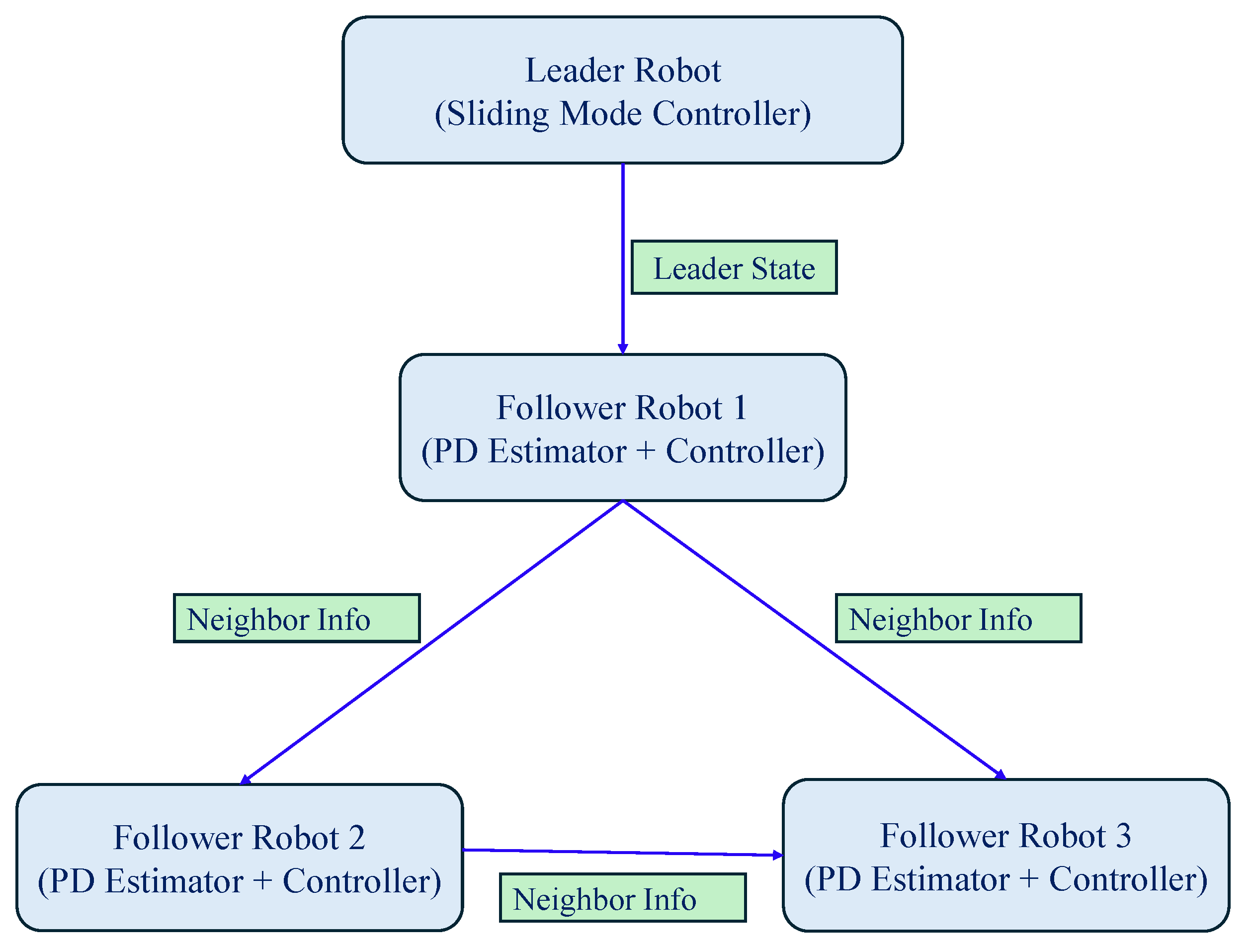
The numerical simulation results were conducted using MATLAB 2021a to demonstrate the efficiency and performance of the proposed formation controllers. Hence, we present the simulation results based on the leader–follower approach using multiple NWMRs. The communication topology among the multiple NWMRs is a directed graph $\mathcal{G}$ which is shown in Figure 4. Moreover, the formation forms a desired pattern by three followers $R_1$, $R_2$, $R_3$, which follow the leader $R_0$. The simulation results are summarized in two sections. The first section demonstrates the results of the leader robot using designed leader control inputs (25). Another section demonstrates the result of multiple followers along with the desired triangular formation using the distributed estimator-based formation controllers (61). The proposed control system parameters, communication models, and robot dynamics are listed in the

Table 2. Summary of system parameters, communication models, and robot dynamics assumptions.

Category	Description / Parameter
System Parameters
Number of Robots	4 (1 leader + 3 followers)
Sampling Time ($T_s$)	0.01 seconds
Control Gains (Leader)	Sliding surface parameters: $k_1=1.5$, $k_2=1.2$
Control Gains (Followers)	PD gains: $K_p=2.0$, $K_d=0.5$
Reference Trajectory	Circular trajectory with radius 5 m, speed 0.3 m/s
Communication Model
Topology	Directed graph (Leader–follower)
Communication Range	Limited to neighboring robots only
Information Access	Followers do not have direct access to leader state
Communication Delay	Neglected/assumed negligible
Robot Dynamics Assumptions
Robot Type	Nonholonomic Wheeled Mobile Robots (NWMRs)
Kinematic Constraints	Standard nonholonomic constraints (no lateral slipping)
Maximum Velocity	Linear velocity $\le 0.5$ m/s, angular velocity $\le 1.0$ rad/s
Disturbances	Small bounded disturbances considered on follower robots

.

Section 1: The leader robot control inputs have been designed by using the reference robot $R_r$’s information. The parameters of the reference robots are as follows. The initial position of the reference robot $R_r$ is ${[23,25,0]}^T$ and the its linear velocity $v_r$ and angular velocity ${\omega }_r$ are set as $(3-(0.25cos\left(0.24t\right)\left)\right)$ and $0.5cos\left(t\right)$, respectively.

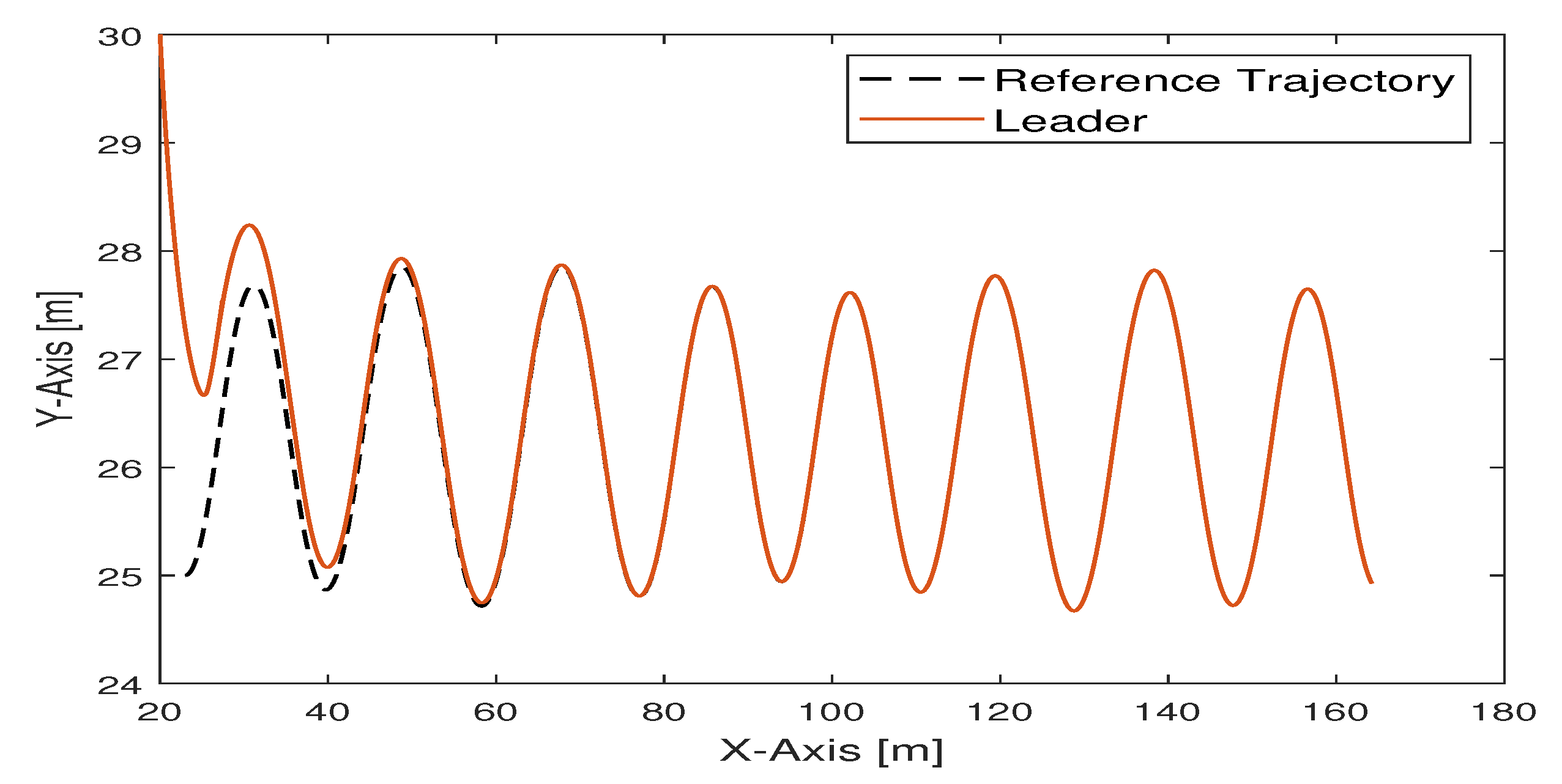
The leader robot $R_0$ starts from the initial position ${[20,30,-1]}^T$. Moreover, we set the control parameter values for the proposed controller as $K_0=1$, $K_3=5$ and $\alpha =5$. We have simulated the leader NWMR system with the tracking controllers (37) and (25) and the obtained results are shown in Figure 6, Figure 7, Figure 8 and Figure 9. From these simulation results, Figure 6 illustrates the trajectory of the leader $R_0$ which follows the trajectory of reference $R_r$. The proposed controllers (37) and (25) guide the leader to follow the reference trajectory when a leader starts from a different position. Figure 7 denotes the tracking error of the $R_0$, which converges to zero over time. Figure 8 shows the linear and angular velocities of robots $R_0$ and $R_r$. Furthermore, the asymptotically convergence of the linear and angular velocity control error is shown in Figure 9.

Section 2: In this work, for the simulation purpose, the formation has been considered for a group of four NWMRs comprised of one leader and three followers, as shown in Figure 4. The values of the three follower initial positions are set as $R_1\left(0\right)={[20,50,-5]}^T$, $R_2\left(0\right)={[-10,30,17]}^T$, and $R_3\left(0\right)={[10,10,-15]}^T$. In addition, the linear and angular velocities of the leader referred to the previously designed controllers (37) and (26). The goal of our method is to develop the desired triangular formation of followers and follow the leader at the desired distance. Therefore, the desired relative distances of the followers are set as ${\Delta }_{x1}=1$, ${\Delta }_{y1}=1$, ${\Delta }_{x2}=4$, ${\Delta }_{y2}=4$, ${\Delta }_{x3}=4$, ${\Delta }_{y3}=2.5$. Due to the communication problem, in this work, we proposed the distributed estimator (43) and its parameters are set to ${\gamma }_i=10$ ${\mu }_1=5$, ${\mu }_2=2$, ${\mu }_3=2$, and ${\mu }_4=2$. Moreover, the control gain of the proposed control laws (69) and (61) are set as $K_1=5$, $K_2=2$, $K_3=20$. 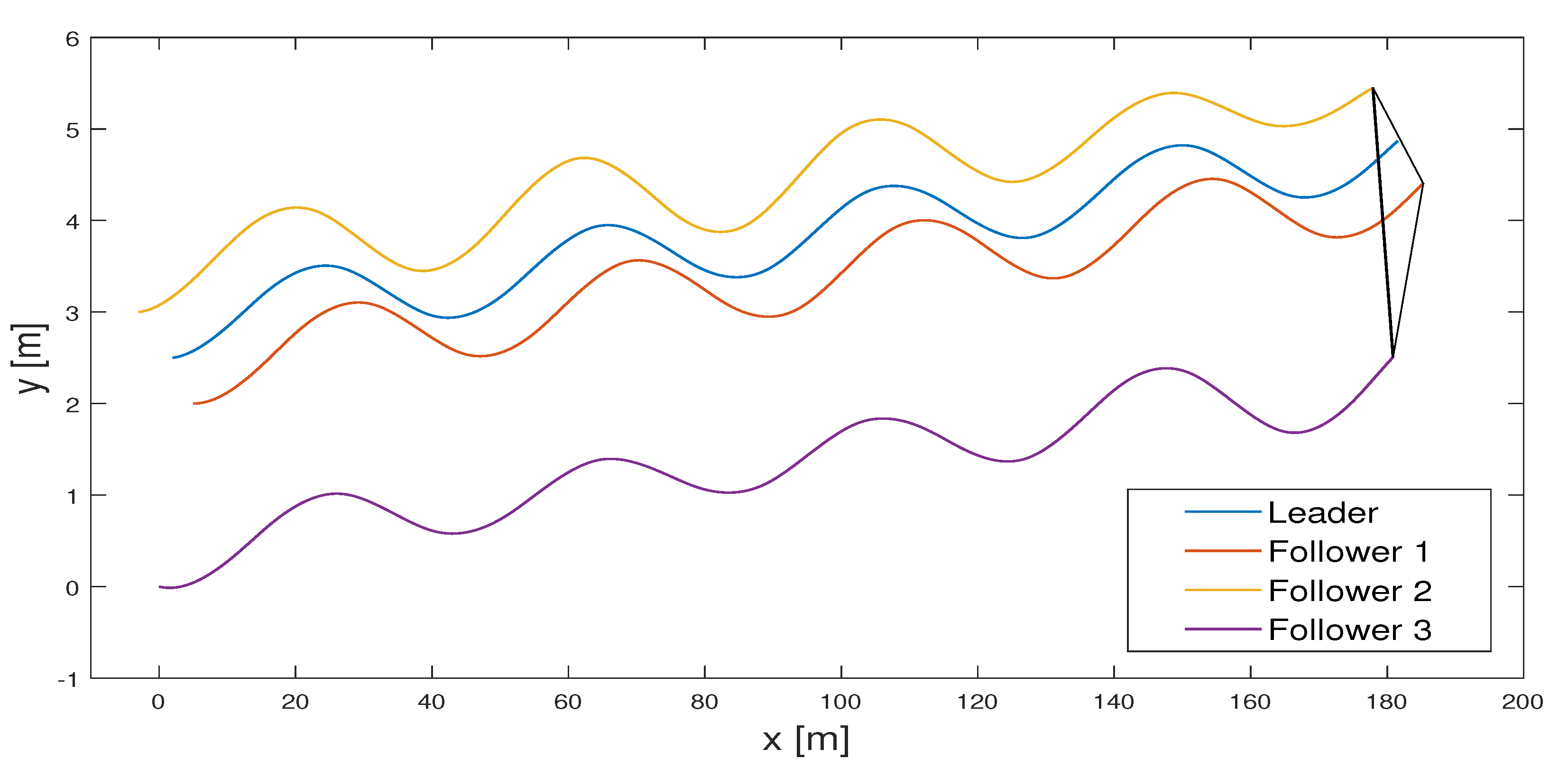The simulation results of the follower’s proposed control strategy are presented in Figure 10, Figure 11, Figure 12, Figure 13, Figure 14 and Figure 15. The trajectory tracking results of multiple NWMRs using the estimators and proposed control laws (37) and (26) are shown in Figure 10, where the desired triangle formation is achieved. Moreover, from Figure 11, we observe that the linear and angular velocity of the estimation error converged to zero. In addition, each follower’s estimator predicts the relative position of the leader, as shown in Figure 12. The estimation error of the proposed estimator (43) is shown in Figure 13, where the tracking errors converge to zero. Based on proposed controllers (37) and (26), the multiple NWMRs can achieve the desired pattern, and the formation tracking error converged to zero means that the control objectives can be achieved. Finally, from the above discussion along with results illustrated in Figure 6, Figure 7, Figure 8, Figure 9, Figure 10, Figure 11, Figure 12, Figure 13, Figure 14 and Figure 15, we conclude that the proposed control schemes are effectively verified.

4.1. Simulation Results on Different Formation Type

We present simulation results for a group of four NMRs including three follower robots and a virtual leader robot. The communication link between the leader and three followers is shown in Figure 5. The main objective is to maintain a triangular formation structure along with the given reference paths. The whole parameters are shown below. The initial states of the follower robots are $R_1\left(0\right)={[5,2,0]}^T$, $R_2\left(0\right)={[-3,3,0.5]}^T$, $R_3\left(0\right)=[0,0,-1]$. The initial state of the leader robot is considered as $R_l\left(0\right)={[2,2.5,0.6]}^T$. Moreover, the control inputs for the leader are set to $v_r\left(t\right)=2-0.3(cost)$ and ${\omega }_r\left(t\right)=cos\left(0.3t\right)$. It can be observed from Figure 16 that the follower NMRs form a triangular structure, which is led by the leader NMR. To show the usefulness of the proposed formation control method, we consider a group of four followers and one virtual leader. The desired geometric pattern is a rectangle. Figure 17 shows the trajectories of all robots during 0–45 s; it can be seen from the graph that the multi-robot system converges to the desired formation pattern gradually.

4.2. Sensitivity Analysis of Control Parameters and Environmental Variations

To evaluate the robustness and generalizability of the proposed distributed leader–follower control strategy, we conducted a comprehensive sensitivity analysis considering variations in leader trajectory, communication delay, and control gains. This analysis aims to demonstrate that the control approach does not overfit specific conditions and can maintain stability and acceptable tracking performance under realistic disturbances.

4.2.1. Effect of Leader Trajectory Variations

To examine the adaptability of the controller to different motion profiles, the leader robot was tested on three trajectory types: (i) a smooth linear trajectory, (ii) a circular trajectory with moderate curvature, and (iii) an aggressive sinusoidal trajectory with high curvature and varying frequency. The follower robots consistently maintained formation and demonstrated low RMSE values across all scenarios. While minor increases in tracking error were observed for the sinusoidal path due to sharp directional changes, the system preserved stability and global asymptotic convergence. These results in Figure 18 confirm that the proposed controller generalizes well and does not rely on trajectory-specific tuning.

4.2.2. Effect of Communication Delay

To simulate real-world communication challenges, we introduced artificial delays into the inter-agent communication links, as shown in Figure 19, with delay values ranging from 0 ms (ideal case) to 200 ms. The control system remained stable under delays up to 100 ms, with only slight degradation in tracking accuracy and increased response time. For a 200 ms delay, transient tracking errors increased marginally, but the follower robots continued to converge to the desired trajectory without violating formation constraints. This indicates that the control law’s local design and reliance on neighbor information confer robustness to moderate latency in communication, a common scenario in distributed robotic systems.

4.2.3. Effect of Control Gain Perturbations

To assess the impact of gain variations on control performance, we perturbed the nominal proportional ($K_p$) and derivative ($K_d$) gains by ±20% and ±40%. The system showed graceful degradation in tracking performance in Figure 20 as gains deviated from their tuned values. Lower gains resulted in slower response and increased steady-state error, while higher gains introduced mild overshoot but improved responsiveness. In all cases, the formation remained intact, and the system avoided instability or oscillations, validating the wide operating margin of the controller and its insensitivity to exact gain tuning. These findings highlight the robustness and practical reliability of the proposed PD-based distributed control framework.

4.3. Ablation Analysis

To assess the contribution of key components in our proposed control architecture, we conducted an ablation study focusing on the roles of the distributed estimator and the PD (Proportional–Derivative) control terms. Specifically, we evaluated system performance under three configurations: (1) the full proposed method with both estimator and PD control; (2) removal of the distributed estimator, where followers rely only on delayed or partial leader information; and (3) removal of PD terms, using a purely proportional controller.

The ablation study plot comparing the tracking error for three controller configurations is shown in Figure 21.

(a)

Proposed Method (Estimator + PD): Lowest and fastest-converging error.

(b)

Without Estimator: Higher error, slower convergence.

(c)

Without D-Term: Moderate performance with slower error decay than the full method.

The results clearly demonstrate that the distributed estimator significantly improves tracking accuracy by mitigating communication delays and estimation uncertainties. Without it, follower robots exhibited larger tracking errors and delayed convergence. Similarly, removing the derivative term led to slower response dynamics and higher overshoot, particularly during sudden trajectory changes or disturbances. These findings validate the necessity of each component and reinforce the design choices made in our control framework.

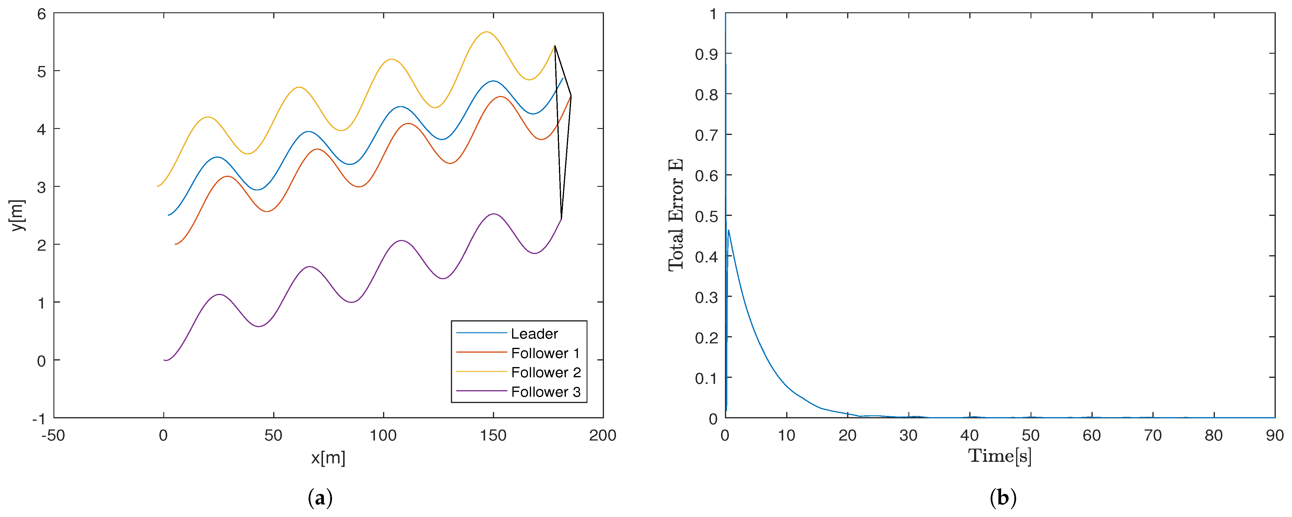
4.4. Comparison with the Distributed Estimator-Based Controllers

A comparative analysis is performed against the control methods presented in [13,18] to highlight the benefits of the proposed formation control strategy. This evaluation is carried out in a leader–follower setup, involving one leader and three follower robots arranged in a triangular formation. To quantitatively evaluate the tracking performance of the formation, the total formation error is defined as

$$E(t)={\left[\sum _{i=1}^3\left(|x_i\left(t\right)-x_r\left(t\right)-{\Delta }_{ix}{|}^2+|y_i\left(t\right)-y_r\left(t\right)-{\Delta }_{iy}{|}^2+{|{\theta }_i\left(t\right)-{\theta }_t\left(t\right)|}^2\right)\right]}^{\frac{1}{2}}.$$

(75)

The performance comparison between the controllers from [18] and the proposed approach is presented in Figure 22, Figure 23 and Figure 24. To ensure a fair evaluation against the method in [13], the same simulation conditions are maintained in Equations (69) and (61). As illustrated in Figure 22, the referenced method delivers a commendable performance; however, it is well known that the backstepping controller may produce large initial velocity spikes and abrupt changes during sudden tracking errors, which limits its practicality for real-world applications. Conversely, the controller proposed in [18] utilizes a distributed observer at each follower robot to estimate the leader’s state. The trajectories generated by this method are depicted in Figure 23, demonstrating successful achievement of the desired triangular formation. Nonetheless, a comparison of the total error plots in Figure 23 and Figure 24 reveals that the controller from [18] experiences considerably higher errors during the initial phase of operation. This reduction in performance is primarily attributed to the initial inaccuracies in leader state estimation, which adversely affect the controller’s early behavior.

The proposed control strategy integrates coordination errors among follower robots directly into its framework, leading to improved accuracy in formation tracking. In contrast to earlier centralized methods, this approach enables formation control of NWMRs within a distributed architecture. This represents a significant progression, as distributed systems inherently provide better scalability, increased resilience to faults, and lower computational and communication loads on the leader. Additionally, simulation outcomes demonstrate that the bioinspired control model successfully mitigates the velocity discontinuities typically observed in backstepping-based controllers, thereby reinforcing the effectiveness of the proposed method.

4.5. Response to Sudden Disturbances

To validate the robustness of the proposed controller under realistic and challenging conditions, we conducted a set of dedicated simulations introducing sudden external disturbances to the system, as shown in Figure 25. These disturbances were designed to mimic unexpected real-world events such as uneven terrain effects, wind gusts, or temporary actuator faults. In the simulation setup, disturbances were introduced in two ways:

(a)

Impulse Disturbances on Leader: A sudden force was applied to the leader robot at $t=15$ s, deviating momentarily from its planned trajectory. The controller successfully compensated for the disturbance within a few seconds, realigning the leader to its intended path. The follower robots, relying on the distributed estimator, adapted to the leader’s corrective motion without compromising the triangular formation.

(b)

Random Lateral Perturbations on Followers: Each follower was subjected to random lateral position offsets (magnitude between 0.5 and 1.0 units) at different time instances (e.g., t = 20 s, 25 s). These perturbations disrupted the formation briefly. However, the PD-based control law, supported by the estimator, promptly corrected the deviations, and the swarm regained the desired formation with minimal tracking error growth.

Figures visualize the following:

• The deviation and recovery trajectories of the leader and followers.
• The corresponding tracking errors during and after disturbances.
• The estimator response to sudden state changes.

These simulations demonstrate that the proposed control strategy exhibits strong disturbance rejection capability, effectively maintaining tracking performance and formation shape under sudden, unpredictable changes in the robot states. This reinforces the practical viability of our approach in dynamic, unstructured environments.

4.6. Comparison with Distributed and Centralized Strategies

To further strengthen the evaluation of the proposed distributed estimator–controller, we conducted a comparative analysis against both centralized and conventional distributed control strategies, as shown in Figure 26. In centralized approaches, a global planner computes and broadcasts commands to all robots, typically offering high coordination accuracy. However, such systems are highly sensitive to communication failures and suffer from scalability limitations. In contrast, our distributed strategy, which leverages local information and estimations of the leader’s trajectory, shows superior robustness in the presence of communication uncertainties and delays.

In our simulation, the proposed method achieved a formation tracking RMSE of 2.6425, 3.0132, and 4.2132 for followers $R_1,R_2$, and $R_3$, respectively. These values are comparable to or better than those observed with centralized control under ideal conditions, but show significantly more resilience when subject to packet loss or network delays. When benchmarked against a basic distributed consensus-based controller without estimation, the proposed method demonstrated faster convergence and smaller steady-state errors, especially when the leader executed dynamic trajectories.

Moreover, the proposed method maintained formation integrity even under sudden disturbances and topology changes, scenarios where the performance of centralized and conventional distributed methods degraded considerably. This indicates that our estimator-based approach offers a favorable trade-off between coordination accuracy and system robustness, particularly in dynamic or partially observable environments. Such performance highlights the method’s suitability for real-world applications requiring autonomy and fault tolerance.

4.7. Limitations of the Proposed Control Scheme

The proposed distributed leader–follower control strategy demonstrates effective trajectory tracking and formation maintenance for small-scale groups of NWMRs; several limitations remain to be addressed for broader applicability. First, scalability to large-scale robot swarms poses a significant challenge. As the number of robots increases, communication overhead and network complexity grow, potentially leading to increased delays and information loss. The current method assumes reliable communication within the modeled topology, and its performance under high network congestion or packet drops requires further investigation. Second, the proposed control framework does not explicitly account for dynamic obstacle avoidance. In practical environments where obstacles may appear unpredictably, integrating real-time sensing and reactive planning mechanisms is essential to ensure safe navigation while preserving formation and tracking objectives. Third, computational complexity and real-time implementation constraints may limit deployment on resource-constrained platforms. Although the distributed nature of the control reduces centralized computation, the sliding mode control law and state estimators require careful tuning and sufficient processing capability to maintain stability and responsiveness. Addressing these limitations through advanced communication protocols, adaptive obstacle avoidance strategies, and computationally efficient algorithms represents a promising direction for future work to enhance the robustness and applicability of the control scheme in complex, real-world multi-robot scenarios.

5. Conclusions

This study presents a distributed formation tracking control strategy for NWMRs using a cascade control framework. The approach integrates a sliding-mode-based tracking controller for the leader robot and a PD-based distributed estimator–controller for the follower robots. The followers estimate the leader’s state using only locally available information from neighboring agents. The overall control strategy is supported by a rigorous stability analysis grounded in the cascade system theory, ensuring uniform global asymptotic stability of the interconnected system. The proposed method demonstrates several strengths, including scalability, robustness to partial or delayed communication, and reduced reliance on centralized coordination. These attributes make the controller suitable for deployment in larger, more dynamic robotic teams operating under constrained communication environments. Simulation results confirm the effectiveness of the proposed strategy in maintaining formation and accurate trajectory tracking. Future work will explore extensions to dynamic multi-robot systems with torque control considerations and will focus on validating the proposed framework through experimental implementation on real robotic platforms.

References

1. Das, A.K.; Fierro, R.; Kumar, V.; Ostrowski, J.P.; Spletzer, J.; Taylor, C.J. A vision-based formation control framework. IEEE Trans. Robot. Autom. 2002, 18, 813–825. [Google Scholar] [CrossRef]
2. Consolini, L.; Morbidi, F.; Prattichizzo, D.; Tosques, M. Leader–follower formation control of nonholonomic mobile robots with input constraints. Automatica 2008, 44, 1343–1349. [Google Scholar] [CrossRef]
3. Park, B.S.; Yoo, S.J. Connectivity-maintaining obstacle avoidance approach for leader-follower formation tracking of uncertain multiple nonholonomic mobile robots. Expert Syst. Appl. 2021, 171, 114589. [Google Scholar] [CrossRef]
4. Jamshidi, M. Autonomous control of complex systems: Robotic applications. Appl. Math. Comput. 2001, 120, 15–29. [Google Scholar] [CrossRef]
5. Yoo, S.J.; Park, B.S. Quantized feedback control strategy for tracking performance guarantee of nonholonomic mobile robots with uncertain nonlinear dynamics. Appl. Math. Comput. 2021, 407, 126349. [Google Scholar] [CrossRef]
6. Ben Hazem, Z.; Guler, N.; Altaif, A.H. A study of advanced mathematical modeling and adaptive control strategies for trajectory tracking in the Mitsubishi RV-2AJ 5-DOF Robotic Arm. Discov. Robot. 2025, 1, 2. [Google Scholar] [CrossRef]
7. Balch, T.; Arkin, R.C. Behavior-based formation control for multirobot teams. IEEE Trans. Robot. Autom. 1998, 14, 926–939. [Google Scholar] [CrossRef]
8. Lewis, M.A.; Tan, K.H. High precision formation control of mobile robots using virtual structures. Auton. Robot. 1997, 4, 387–403. [Google Scholar] [CrossRef]
9. Do, K.D. Formation tracking control of unicycle-type mobile robots with limited sensing ranges. IEEE Trans. Control Syst. Technol. 2008, 16, 527–538. [Google Scholar] [CrossRef]
10. Sudhakara, P.; Ganapathy, V.; Priyadharshini, B.; Sundaran, K. Obstacle avoidance and navigation planning of a wheeled mobile robot using amended artificial potential field method. Procedia Comput. Sci. 2018, 133, 998–1004. [Google Scholar] [CrossRef]
11. Peng, Z.; Wen, G.; Rahmani, A.; Yu, Y. Leader–follower formation control of nonholonomic mobile robots based on a bioinspired neurodynamic based approach. Robot. Auton. Syst. 2013, 61, 988–996. [Google Scholar] [CrossRef]
12. Liu, T.; Jiang, Z.P. Distributed formation control of nonholonomic mobile robots without global position measurements. Automatica 2013, 49, 592–600. [Google Scholar] [CrossRef]
13. Yu, X.; Liu, L. Distributed formation control of nonholonomic vehicles subject to velocity constraints. IEEE Trans. Ind. Electron. 2015, 63, 1289–1298. [Google Scholar] [CrossRef]
14. Peng, Z.; Yang, S.; Wen, G.; Rahmani, A.; Yu, Y. Adaptive distributed formation control for multiple nonholonomic wheeled mobile robots. Neurocomputing 2016, 173, 1485–1494. [Google Scholar] [CrossRef]
15. Lu, P.; Wang, H.; Zhang, F.; Yu, W.; Chen, G. Formation control of nonholonomic mobile robots using distributed estimators. IEEE Trans. Circuits Syst. II Express Briefs 2020, 67, 3162–3166. [Google Scholar] [CrossRef]
16. Hou, R.; Cui, L.; Bu, X.; Yang, J. Distributed formation control for multiple non-holonomic wheeled mobile robots with velocity constraint by using improved data-driven iterative learning. Appl. Math. Comput. 2021, 395, 125829. [Google Scholar] [CrossRef]
17. Zhang, H.; Sun, J.; Wang, Z. Distributed Control of Nonholonomic Robots Without Global Position Measurements Subject to Unknown Slippage Constraints. IEEE/CAA J. Autom. Sin. 2021, 9, 354–364. [Google Scholar] [CrossRef]
18. Moorthy, S.; Joo, Y.H. Distributed Leader-Following Formation Control for Multiple Nonholonomic Mobile Robots via Bioinspired Neurodynamic Approach. Neurocomputing 2022, 492, 308–321. [Google Scholar] [CrossRef]
19. Moorthy, S.; Kuppusami Sakthivel, S.S.; Joo, Y.H.; Jeong, J.H. Distributed Observer-Based Adaptive Trajectory Tracking and Formation Control for the Swarm of Nonholonomic Mobile Robots with Unknown Wheel Slippage. Mathematics 2025, 13, 1628. [Google Scholar] [CrossRef]
20. Zhang, Y.; Liu, G.; Luo, B. Finite-time cascaded tracking control approach for mobile robots. Inf. Sci. 2014, 284, 31–43. [Google Scholar] [CrossRef]
21. Wang, H.; Zhang, Y.; Wang, X.; Feng, Y. Cascaded continuous sliding mode control for tracked mobile robot via nonlinear disturbance observer. Comput. Electr. Eng. 2022, 97, 107579. [Google Scholar] [CrossRef]
22. Khalil, H. Nonlinear Systems; Pearson Education; Prentice Hall: London, UK, 2002. [Google Scholar]
23. Liu, W.; Wang, X.; Liang, S. Trajectory tracking control for wheeled mobile robots based on a cascaded system control method. In Proceedings of the IECON 2020 The 46th Annual Conference of the IEEE Industrial Electronics Society, Singapore, 18–21 October 2020; IEEE: New York, NY, USA, 2020; pp. 396–401. [Google Scholar]
24. Lewis, F.; Zhang, H.; Hengster-Movric, K.; Das, A. Cooperative Control of Multi-Agent Systems: Optimal and Adaptive Design Approaches; Communications and Control Engineering; Springer: London, UK, 2014. [Google Scholar]
25. Li, S.; Tian, Y.P. Finite-time stability of cascaded time-varying systems. Int. J. Control 2007, 80, 646–657. [Google Scholar] [CrossRef]
26. Ou, M.; Li, S.; Wang, C. Finite-time tracking control for nonholonomic mobile robots based on visual servoing. Asian J. Control. 2014, 16, 679–691. [Google Scholar] [CrossRef]
27. Wen, G.; Yu, W.; Chen, M.Z.; Yu, X.; Chen, G. Pinning a complex network to follow a target system with predesigned control inputs. IEEE Trans. Syst. Man Cybern. Syst. 2018, 50, 2293–2304. [Google Scholar] [CrossRef]
Figure 1. Cascade interconnection of two subsystems.
Robotics 14 00088 g001
Figure 2. Kinematic model of the NWMR.
Robotics 14 00088 g002
Figure 3. The leader–follower formation framework.
Robotics 14 00088 g003
Figure 4. Communication graph among the multiple robots.
Robotics 14 00088 g004
Figure 5. Control system block diagram of the proposed leader–follower framework for NMRs.
Robotics 14 00088 g005
Figure 6. Two-dimensional trajectory tracking of reference and leader robot.
Robotics 14 00088 g006
Figure 7. Tracking error between reference and leader. Figure (a) x-axis error, (b) y-axis error, and (c) angular error.
Robotics 14 00088 g007
Figure 8. Linear and angular velocity of reference and leader. Figure (a) linear velocity, (b) angular Velocity.
Robotics 14 00088 g008
Figure 9. Linear and angular velocity error of reference and leader. Figure (a) linear velocity, (b) angular Velocity.
Robotics 14 00088 g009
Figure 10. Formation tracking of all robots.
Robotics 14 00088 g010
Figure 11. Linear and angular velocity error of leader and followers. Figure (a) linear velocity and (b) angular velocity.
Robotics 14 00088 g011
Figure 12. The trajectory of the leader and the three estimators in the x, y, and θ coordinate axes. Figure (a) x-axis trajectory, (b) y-axis trajectory, and (c) angular trajectory.
Robotics 14 00088 g012
Figure 13. Evolution of estimation error. Figure (a) x-axis error, (b) y-axis error, and (c) angular error.
Robotics 14 00088 g013
Figure 14. Tracking error of leader and the three followers. Figure (a) x-axis error, (b) y-axis error, and (c) angular error.
Robotics 14 00088 g014
Figure 15. Linear and angular velocity of leader and followers. Figure (a) linear velocity and (b) angular velocity.
Robotics 14 00088 g015
Figure 16. Trajectories of the leader NMR and the follower NMRs.
Robotics 14 00088 g016
Figure 17. Trajectories of the leader NMR and the follower NMRs.
Robotics 14 00088 g017
Figure 18. Leader and follower trajectories.
Robotics 14 00088 g018
Figure 19. Tracking error vs. time for communication delays.
Robotics 14 00088 g019
Figure 20. RMSE vs. Control Gain Variations.
Robotics 14 00088 g020
Figure 21. Ablation study plot comparing the tracking error.
Robotics 14 00088 g021
Figure 22. Comparison results among the controllers in [13]. (a) Robot position with the controller in [13]. (b) Total error with the controller in [13].
Robotics 14 00088 g022
Figure 23. Comparison results among the controllers in [18]. (a) Robot position with the controller in [18]. (b) Total error with the controller in [18].
Robotics 14 00088 g023
Figure 24. Results among the controllers in the proposed method. (a) Robot position with the proposed controller. (b) Total error with the proposed controller.
Robotics 14 00088 g024
Figure 25. Leader and follower robots respond to sudden disturbances.
Robotics 14 00088 g025
Figure 26. Comparison of tracking RMSE across control strategies.
Robotics 14 00088 g026