Abstract
The Euler–Lagrange and Newton–Euler methods are typically used to derive equations of motion for serial-link manipulators. We previously proposed a partial Lagrangian method, which is similar to the Lagrangian method, for handling the equations of motion analytically. Moreover, the proposed method can efficiently handle multi-link analyses, similar to the Newton–Euler method. The partial Lagrangian method organizes the Lagrangian, which is obtained from the link structure, and torque, which is obtained by differential operations, into a table that can be easily handled by both manual calculations and computer analysis. Furthermore, by representing it using a computational graph, it is possible to perform dynamic analysis while maintaining the structure of a system. By observing the intermediate nodes of this computational graph, it is possible to observe how the torque generated at a particular link affects the joint. Organizing the structure with graphs allows us to consider complex systems as a collection of subgraphs, making this method highly compatible with our proposed partial Lagrangian approach. This study shows that the partial torque tensor can be used as an analog of the partial torque table for serial-link systems by interpreting the meaning of the table, i.e., the partial torque, as the interaction between the links in order to simplify the treatment of branching link systems. Due to the use of the partial torque tensor, the dimensions of the tensor correspond one-to-one with the number of branches, allowing the description of any branching system. Furthermore, by using the proposed building block representation, even complex branching systems can be easily designed and analyzed.
1. Introduction
In dynamics, the Newton–Euler and Lagrange methods are well-known for formulating and calculating the equations of motion [1,2,3,4]. The Newton–Euler method describes the mechanical action between adjacent joints. The recursive Newton–Euler algorithm (RNEA) is an algorithm that can systematically calculate one degree of freedom at a time, even in multi-degree-of-freedom models [5,6,7]. The RNEA is an extremely computationally efficient method. We also utilize it for the musculoskeletal dynamics analysis of the human body in our embedded systems [8]. However, while it is a suitable method for obtaining numerical solutions, obtaining analytical solutions requires following very complex procedures due to the nature of sequential calculations. Conversely, the Lagrange method is a formulation procedure that yields analytical solutions that can be understood in physically meaningful terms. However, analyzing multi-DoF systems incurs a significant computational burden. Therefore, they are typically used for analyzing systems with fewer DoFs.
We previously proposed a partial Lagrangian method for handling the equations of motion analytically, similar to the Lagrangian method; however, it can efficiently handle multi-link analysis, similar to the Newton–Euler method [9]. The partial Lagrangian method organizes the Lagrangian, which is obtained from the link structure, and the torque, which is obtained by differential operations, into a table that can be handled easily by both manual calculations and computer analysis.
The partial Lagrangian method abstracted and organized the formula structure of the serial-link manipulator, wherein the extension and reduction of links corresponded to the addition and deletion of columns in the upper triangular matrix and partial torque table. Extending this idea to capture the abstract link structure can enable branching link systems to be treated as analogs of serial-link systems by considering the matrix as a tensor.
In contrast to serial link manipulators, which are common in conventional industrial robots, these robots can handle complex tasks due to their complex branched joint structures. For example, in recent years, the development of robots with human-like arms and legs has rapidly progressed, including dual-arm robots for cooperative tasks [10,11,12] and more versatile humanoid robots [13,14,15]. Studies of robots with more complex shapes are also active, including the multi-legged robot [16,17,18], which is good at moving over uneven terrain. As Featherstone points out, dealing with branches and kinematic loops is an important aspect of applying analytical algorithms to complex systems [19]. As mentioned above, the RNEA, based on the Newton–Euler method, is an efficient computational method and is used in many studies on robotic systems to calculate joint torques. However, our goal is to analyze in detail how the behavior of a particular link affects each joint. This information is useful when analyzing complex human structures. For a detailed analysis of such dynamic effects, we focus on a branch method that uses the Lagrangian equations as the fundamental equations and maintains the structure of the equations by using a computational graph.
This study showed that the partial torque tensor can be used as an analog of the partial torque table for serial-link systems by interpreting the meaning of the table, i.e., the partial torque, as the interaction between the links in order to simplify the treatment of branching link systems.
2. Methods
We are focusing on methods for handling multi-degree-of-freedom systems as a first step, with the ultimate goal of performing dynamics analysis of complex systems such as humans. In addition, a particular point of view we wish to focus on is the analytical determination of the effects that variations in one part of the system have on the others. Therefore, Lagrange’s equation is employed as the fundamental equation for handling the analytical solution of the equation of motion. We have previously proposed a partial Lagrangian based on Lagrange’s equation with a divide-and-conquer approach as a method for analyzing the mechanical impact of each link on the others [9]. Another unique feature of our approach is the use of automatic differentiation, a tool used in AI learning, for the analysis. The differential operations of Lagrange’s equations correspond to the gradient calculations in a computation graph. By converting the energy balance into a computation graph, we can perform dynamic analysis. Therefore, the computation graph is very suitable for the Lagrangian approach. Furthermore, automatic differentiation can preserve the analytical solution structure in the form of a graph structure called a computational graph, which allows for the analysis of dynamical effects from the connection relations of the graphs.
In Section 2.1, the idea of splitting into partial Lagrangians is described using a simple example. Section 2.2 describes the preservation of the expression structure of partial Lagrangians by automatic differentiation and its analysis based on gradient calculations. Section 2.3 describes how to extend our proposed method to branched systems.
2.1. Partial Lagrangian and Partial Torque
The partial Lagrangian method uses the divide-and-conquer approach [20,21] for dividing the equations of motion, which become complex when the number of DoF increases into the smallest units. Specifically, we consider the partial Lagrangian for each link instead of the Lagrangian of the entire system, based on the following equation.
Here, we consider a planar serial link manipulator. n represents the number of links, the denote the kinetic energy, and the denote the potential energy of the i-th link. The use of a partial Lagrangian reduces the computational load because the terms in the equations of motion for extending the number of links can be treated independently. In other words, a similar division process can be performed for each link, and the results can be integrated to obtain an exact analytical solution.
The partial Lagrangian method considers the equations of motion while decomposing the link structure. The equation of motion using the Lagrangian method can be expressed as
where and represent the kth generalized coordinates and force, respectively, and represents the Lagrangian of the entire system.
In the partial Lagrangian method, the differential operator that transforms the Lagrangian into an equation of motion is denoted by D. That is, the operator from which the equation of motion for the kth DoF is derived as follows: . Using this operator, the equation of motion can be written as the sum of the partial torques as
where represents the partial Lagrangian of link i that can be defined as the difference between the kinetic energy and potential energy for the ith link, as mentioned above. This decomposition is a feature of the partial Lagrangian method and shows that even if the partial torques are considered individually, the results of the Lagrangian method are in analytical agreement with the calculated results.
The partial torque is summarized in Table 1, where the properties of the following equation indicate that only the upper triangular part must be calculated.

Table 1.
Partial torque table derived from partial Lagrangian for n-DoF system.
2.2. Dynamics Analysis Based on Computatoinal Graph
We use a computational graph as the preferred method for analyzing partial Lagrangian dynamics. The computational graph allows us to perform the dynamics analysis while preserving the structure of the system. With this computational graph, it is possible to analyze how the movement of a given link has affected the respective joint torques as a result of the action. With this calculated graph, it is possible to analyze the extent to which each joint torque has been affected by the motion of a certain link. This means that computational graph allows direct observation of the aforementioned partial torques.
Furthermore, by using a computational graph, we can calculate the gradients of parameters through automatic differentiation [22]. Automatic differentiation has recently been used in AI learning and is an important concept alongside numerical differentiation and symbolic differentiation [23,24]. Since this gradient calculation is equivalent to finding the differential coefficients, the computational graph can be treated as a differential equation, a balance of energies, without having to transform Lagrange’s equation into a force dimension. Automatic differentiation is primarily a tool used for training AI, and its most important feature is that it performs gradient calculations on computational graphs. Automatic differentiation eliminates the need for complex differential transformations of Lagrange’s equations, making the Lagrangian method easily applicable to complex systems.
Decomposition into partial Lagrangians implies decomposition of the computational graph of automatic differentiation. Compact computational graphs help reduce the load on the analysis and parallelize it. Therefore, the combination of these factors allows for effective analysis of multi-degree-of-freedom systems. Figure 1 shows a conceptual diagram of a dynamics analysis based on Lagrange’s equation, using a computational graph. While the final computational complexity is the same as that of the Lagrangian equations, organizing them as partial torques allows the computational graph of the partial torques to be parallelized [9]. Since the computational graph is automatically generated, we do not need to calculate the differential equations ourselves and derive the equations of motion in the force dimension. Additionally, we focus on the partial torques that appear in the intermediate steps of the computational graph to analyze the impact of motion. Extracting these partial torques is straightforward through the tracing of the nodes of the computational graph.
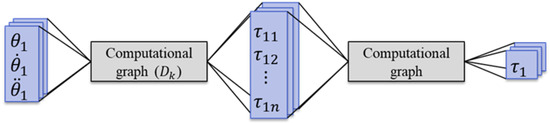
Figure 1.
Concept of analyzing partial torques using automatic differentiation.
Since the equations of motion are described as a computational graph, this can be applied to both inverse dynamics analysis and forward dynamics analysis. An example of analysis by automatic differentiation is shown in Figure 2. Here is a simple example: the free fall of a double pendulum. We assigned subscript 1 to link 1 and subscript 2 to link 2. The physical parameters are as follows: link lengths , , masses , , and damping coefficients , . In order to confirm the validity of the analysis method using automatic differentiation, a comparison with a physics simulator (Mujoco, DeepMind Technologies Ltd., London, UK) is shown. The double pendulum is sensitive to initial conditions, and it is challenging to perfectly match all conditions with the physics simulator. However, as shown in Figure 2, a reasonable simulation has been achieved using inverse dynamics analysis with automatic differentiation and time-stepping with the Runge–Kutta method.
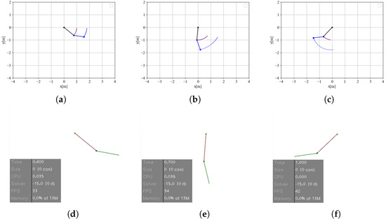
Figure 2.
A simple example of dynamics analysis using automatic differentiation (AD) (a–c) and a comparison with physics engine (PE) simulation (d–f). Analyzing with AD . (b) Analyzing with AD . (c) Analyzing with AD . (d) Simulating with PE . (e) Simulating with PE . (f) Simulating with PE . The red and blue dotted lines represent the trajectories of the ends of each link in (a–c).
2.3. Analysis of Branching System Using Partial Torque Tensor
Based on the partial torque table, a partial Lagrangian is added to the column because of the presence of an additional link. is constructed as the sum of the partial torques , whereas appears because of . The partial torque can be considered as the torque generated by the i-th link and acting on the k-th joint.
Partial torques for the serial-link manipulators are summarized in a table. If this is considered as a partial torque matrix, the analogy is that the matrix can be considered to expand into multiple dimensions in the case of a branched link. This is defined as the partial torque tensor.
An example of the partial torque tensor, compared to the partial torque matrix of the serial link system, is shown in Figure 3. In tensor notation, the branch number is added as a dimension of the tensor. For example, represents the torque generated by the 2nd link and acting on the 1st joint in branch . For the differential operator and the partial Lagrangian , the symbol representing the branch is indicated on the left superscript.Looking at Figure 3b, the system branching into two can be considered as having components of a tensor with two planes.
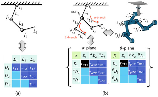
Figure 3.
Relationship between the partial torque matrix and tensor for serial and branched system, respectively. The dimensions of the tensor correspond to the number of branches. (a) Partial torque matrix for serial system. (b) Partial torque tensor for branched system.
However, the black parts in the figure are placed on each plane as tensors, but physically, it means the same torque. In other words, . In tensor notation, the dimensions of the tensor correspond to the number of branches, making it possible to represent branching systems. However, it includes redundant elements. Furthermore, it is difficult to intuitively understand the structure of the system from the shape of the tensor. Additionally, it is difficult to intuitively determine which partial torques should be summed to calculate the joint torque.
2.4. Building Block Representation
As a solution to the aforementioned issues with tensor notation, we propose a block representation. The concept of the building block representation is illustrated in Figure 4. The blocks on the right side of the figure correspond to the partial torque table, with each block representing an element of the partial torque. represents the joint, and there is a corresponding partial differential operator . Figure 4a shows that the torque analysis of a conventional serial link manipulator can be organized using a building block representation of the partial torque table. The partial torque tensor can be expressed as shown in Figure 4b by extending this concept. In this case, we consider an example with a single branch with an branch on one side and a branch on the other as the simplest example.
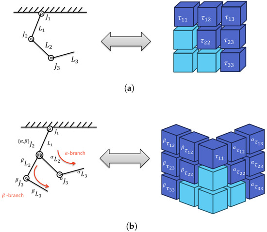
Figure 4.
Branching systems can be considered as an analogy for serial link system using the partial Lagrange method ( refers to the joint and refers to the link’s partial Lagrangian). (a) Serial link systems are mapped to a partial torque table (matrix ). (b) Branching systems are mapped to a partial torque tensor (The right side corresponds to the branch and the left side corresponds to the branch).
The existence of the branch causes link 1 () to change its dynamics. This corresponds to the extension of the matrix to a tensor in the -direction, as shown in Figure 4. The effects of the branched links are consolidated into the 1st link, so in the building block representation, this is depicted by connecting those points. Therefore, in tensor notation, considering the planes for each dimension of the tensor results in redundant representations at the root of the branches. However, in building block representation, intuitive dimensional expansion is possible.
To more intuitively understand the link structure as an analogy to the serial link system, the dimensions of the tensor representing the branches are displayed as the left superscript. In other words, by denoting the partial torque on branch as , we explicitly indicate the branch’s calculation that is being performed. Joint is subject to the action of all forces of the and branches. In , the branch and branch are independent, so the partial torques are as follows:
Here, the left superscript indicates the branch that must be appropriately determined from the tensor structure (link structure). In the case of building block representation, it is possible to determine geometrically whether the blocks are connected. If there is no bifurcation, such as , no subscript is present. However, the forces from all branches are concentrated at this joint. For each branch of and , we must show the branching structure as , which can be considered independent because there are no nonlocal interacting forces.
Only the sum of the slices in the k-direction of the tensor is considered in the calculation of the kth joint torque from the partial torque.
At the joints where the action forces are aggregated, it is sufficient to take the sum of all forces. This can be determined by the adjacency of the tensor elements of the building block representation. Each branch can be calculated independently, except for the base displacements because there is no non-contact force, and the action between the branches is concentrated in the base displacements resulting from the action of the forces on the base joints. The conceptual diagram is shown in Figure 5.
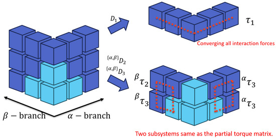
Figure 5.
Concept of joint torque calculation by partial torque tensor.
3. Experiment and Results
As the simplest example, we simulated the branched double pendulums. We consider the normal double pendulum as an branch and add a branch to the branched double pendulum. The parameters used in the simulation were as follows: the 1st link had a length of and a mass of , and a damping coefficient of the joint was set to . For the branch, we used , , , , , . Similarly, for the branch, we used , , , , , . All the centers of mass of the links are located in the middle of the links. In the simulation, a computational graph is created using partial Lagrangians, and the equations of motion are handled through automatic differentiation. Furthermore, by using automatic differentiation in the computational graph, we can automatically determine the articulated-body inertia [25]. This allows for the analysis of system behavior based on the computational graph.
The description and analysis of this system uses our proposed method of automatic differentiation. The partial torque tensor can be handled in its original form by describing the partial Lagrangian as a computational graph, thereby simplifying the system description and analysis. The simulation results are presented in Figure 6. Figure 6a–c show the time evolution immediately after the initial state, while Figure 6d–f show the latter half of the simulation, only before stopping, because of friction damping.
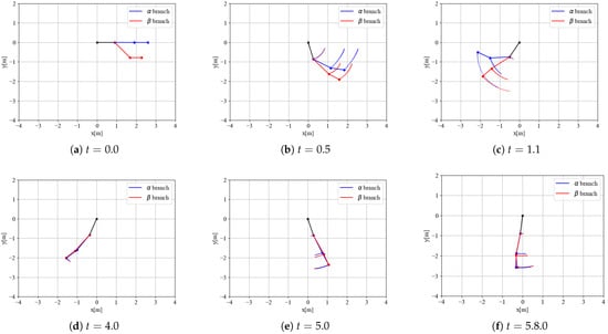
Figure 6.
Simulation results of the branched pendulums. Black, blue, and red colors represent 1st link, branch, and branch, respectively. t represents the timing of the analysis, and the trajectory is displayed with a dotted line.
The and branches are set up independently, which indicates that the mobement of the branch affect the behavior of the connected 1st link, which changes the behavior of the branch.
The building block representation of the partial torque tensor used in the simulation is shown in Figure 7. In this figure, the color intensity indicates the magnitude of the torque, and magenta and cyan indicate the positive and negative torque, respectively. The right and left sides indicate the and branches, respectively. In other words, there are eleven blocks in the diagram, with the center cube representing , the right side representing , and the left side representing . Further, represents the torque produced at the joint by the motion of the branch and represents the torque produced at the joint by the motion of the branch.
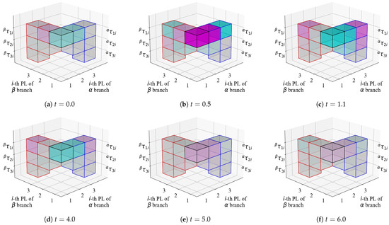
Figure 7.
The partial torque tensors of the branched pendulum are shown for the and branches. The blue and red boxes represent the and branches, respectively. The timing is the same as in Figure 6, and the magenta and cyan colors indicate positive and negative torque, respectively. Darker colors represent larger torques. “i-th PL” means partial Lagrangian of i-th link.
In the initial states (a), the links of branch tend to rotate clockwise under the influence of gravity, resulting in a negative torque. However, a positive torque is generated at , causing movement in the direction of joint extension. At timing (b), each end effector is accelerating, while the movement of the intermediate links is decelerating. At timing (c), the branch is swung up and nearly stationary. Similarly, for the latter timings (d) to (f), we observe a change in the torque produced in by the motion of each branch. In the latter part of the model, the motion is about to stop because of frictional damping; however, the influence of the branch, which has a higher mass, is still strong and appears to drive the entire system.
The building block representation of the partial torque tensor enabled the system to be designed in an abstract manner, and the changes in behavior caused by force transmission were confirmed by simulation. Additionally, by describing and analyzing the system using the partial Lagrangian method, it is possible to perform the analysis simply by adding the partial Lagrangian to the computational graph. The computational graph can perform gradient calculations through automatic differentiation, allowing the automatic derivation of equations of motion. Additionally, by focusing on the partial torque within the computational graph, it is possible to understand the mechanical influence that a particular link exerts on other joints.
4. Discussion
4.1. Extensibility to Multi-Branch Structures
This time, we considered one of the simplest branches (), so Figure 4 could be visualized as a cube. However, because is designed as a tensor, the partial torque tensor becomes multidimensional when extended to multiple branches () and can be treated in the same manner as in the present analysis. This concept is illustrated in Figure 8. In this figure, the final link of the branch is deleted and a new branch link is added. The building block representation of the partial torque tensor enables considering the dynamics of such a complex system by rearranging its connections in an intuitive manner.
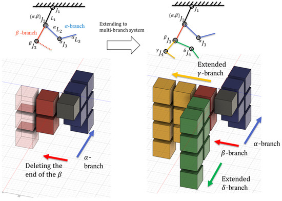
Figure 8.
Concept of extending to multi-branching system by a partial torque tensor.
The organization of the system by tensors is compatible with the parallel dynamic analysis of partial Lagrangian methods conducted using the automatic differentiation that we use [9]. By generating a computational graph through automatic differentiation, it is possible to perform gradient calculations using the balance of the partial differential equation as a constraint. Automatic differentiation is a technique used for gradient calculations in machine learning, but it is also applied in FEM analysis [26,27], dynamics [28,29], and electronic circuit analysis [30,31,32]. In the partial Lagrangian method, it is possible to handle the equations of motion in the form of differential equations by utilizing automatic differentiation, and furthermore, parallel computation for each partial torque is possible. Treating partial torques as tensor elements, as proposed in this method, contributes to compactly organizing the computational graph and allows for handling changes to the system. Therefore, even if the branches become multiple branches or the system branches in the middle over time, any branching system can be analyzed by freely expanding the shape of the partial torque tensors.
4.2. Partial Torque Tensors as Subgraph of Computational Graph
Figure 4 shows that a majority of the partial torque tensors are sparse. When the contents of the partial torque tensor are written in the partial torque table, as shown in Table 2, it confirms that there are many zero elements. Here, the left superscript indicates the branches to be traversed. Differential operators act on the corresponding subscripted partial Lagrangian . Thus, the relationship between links is an important indicator of the transmission of forces. When the partial Lagrangian method is applied to physical systems with nonlocal effects such as Coulomb forces in electromagnetism or gravity, the partial torque tensor is considered dense for nonlocal interactions.
Table 2.
Components of the partial torque tensor of Figure 8 as a partial torque table.
It is not intuitive to describe the partial torque table as a large table; however, if we consider them as a superposition of each branch from the root to the tip, we can decompose them into smaller tables, as indicated in Table 3. The dynamics of the manipulator have no non-contact forces other than gravity, which implies that they can be interpreted as a simple superposition of serial links. In other words, this corresponds to each dimension of the partial torque tensor. Although the conventional Lagrangian method is very difficult to analytically handle large systems as shown in Table 3, the divide-and-conquer approach of the partial Lagrangian method allows complex systems to be organized into combinations of simpler systems.
Table 3.
Decomposition from branching structure to non-branching structure from the perspective of partial torque tensors.
The decomposition of this table from the perspective of the computational graph means decomposing each branch into subgraphs by taking the intermediate state partial torque as the nodes. This conceptual diagram is shown in Figure 9. Although there are other methods of organizing the table, expressing it as a superposition of serial links based on partial torques, as shown in the example, makes it very easy to handle as a computational graph. Additionally, it clearly describes the meaning of the partial torques as the interaction forces we are focusing on. In the figure, the common partial torques corresponding to the table are explicitly shown to represent the branches, but in practice, multiple calculations are unnecessary. Therefore, the building block representation, which can overlap common parts, can be seen as a non-redundant representation of branches.
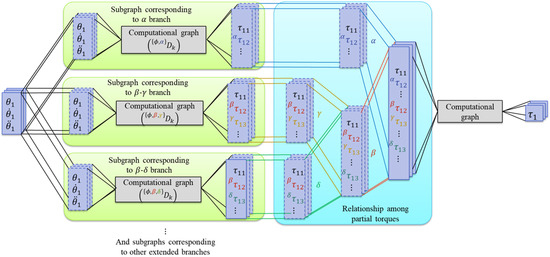
Figure 9.
Partial torque table represented as subgraphs corresponding to Figure 8. Dashed boxes indicate correspondences, while calculations are required for the solid box sections.
By establishing a one-to-one correspondence between the building block representation and the subgraphs of the computational graph, this method can be applied to more complex systems. In future work, we will expand our approach to closed links and three-dimensional motions, referencing the concept of branch-induced sparsity [25].
5. Conclusions
We proposed a partial torque tensor for branching-structured systems by extending the partial Lagrangian method. The partial torque tensor allows the link structures to be abstracted and treated as blocks, thereby enabling the complex link structures to correspond to tensor structures. Furthermore, the partial Lagrangian method can be used to decompose complex tensors and be treated as combinations of simple structures. In this paper, we analyzed a pendulum that branches midway as the simplest branching link. The proposed method enabled the simulation of force interactions, which were caused by the connection of other links, and the dynamic analysis of the branched system.
The proposed method analyzed the dynamics of complex structures by abstracting the link structure and ignoring the complexity of the equations. The analytical accuracy was supported by the Lagrangian method. In addition, only fully abstracted structures could be analyzed by incorporating analytical methods for automatic differentiation. Therefore, our future work will include applications to the more complex systems treated, such as the closed-link systems and the parallel-link systems, in order to verify the versatility of the method.
Author Contributions
Conceptualization, T.K.; investigation, T.K.; methodology, T.K.; supervision, T.T.; validation, T.K. and T.T.; writing—original draft, T.K.; writing—review and editing, T.T. All authors have read and agreed to the published version of the manuscript.
Funding
This study was partially supported by the JSPS KAKENHI Grant Number JP22H01436.
Institutional Review Board Statement
Not applicable.
Informed Consent Statement
Not applicable.
Data Availability Statement
Data are contained within the article.
Acknowledgments
The authors gratefully acknowledge support from the JSPS KAKENHI.
Conflicts of Interest
The authors declare no conflicts of interest.
References
- de Jesus Rubio, J.; Humberto Perez Cruz, J.; Zamudio, Z.J.; Salinas, A. Comparison of two quadrotor dynamic models. IEEE Lat. Am. Trans. 2014, 12, 531–537. [Google Scholar] [CrossRef]
- Ali, S. Newton-Euler Approach for Bio-Robotics Locomotion Dynamics: From Discrete to Continuous Systems. Ecole des Mines de Nantes, 2011. English. NNT: 2011EMNA0001. tel-00669588. Available online: https://theses.hal.science/tel-00669588/ (accessed on 21 December 2024).
- Sciavicco, L.; Siciliano, B.; Luigi, V. Lagrange and Newton-Euler dynamic modeling of a gear-driven robot manipulator with inclusion of motor inertia effects. Adv. Robot. 1995, 10, 317–334. [Google Scholar] [CrossRef]
- Robotic Systems Lab, ETH Zurich Robot Dynamics Lecture Notes. 2017. Available online: https://ethz.ch/content/dam/ethz/special-interest/mavt/robotics-n-intelligent-systems/rsl-dam/documents/RobotDynamics2017/RD_HS2017script.pdf (accessed on 20 September 2022).
- De Luca, A.; Ferrajoli, L. A modified newton-euler method for dynamic computations in robot fault detection and control. In Proceedings of the 2009 IEEE International Conference on Robotics and Automation, Kobe, Japan, 12–17 May 2009; pp. 3359–3364. [Google Scholar] [CrossRef]
- Buondonno, G.; De Luca, A. A recursive Newton-Euler algorithm for robots with elastic joints and its application to control. In Proceedings of the 2015 IEEE/RSJ International Conference on Intelligent Robots and Systems (IROS), Hamburg, Germany, 28 September–3 October 2015; pp. 5526–5532. [Google Scholar] [CrossRef]
- Li, X.; Nishiguchi, J.; Minami, M.; Matsuno, T.; Yanou, A. Iterative calculation method for constraint motion by extended newton-euler method and application for forward dynamics. In Proceedings of the 2015 IEEE/SICE International Symposium on System Integration (SII), Nagoya, Japan, 11–13 December 2015; pp. 313–319. [Google Scholar] [CrossRef]
- Tsuchiya, Y.; Imamura, Y.; Tanaka, T.; Kusaka, T. Estimating Lumbar Load During Motion with an Unknown External Load Based on Back Muscle Activity Measured with a Muscle Stiffness Sensor. J. Robot. Mechatron. 2018, 30, 696–705. [Google Scholar] [CrossRef]
- Kusaka, T.; Tanaka, T. Partial Lagrangian for Efficient Extension and Reconstruction of Multi-DoF Systems and Efficient Analysis Using Automatic Differentiation. Robotics 2022, 11, 149. [Google Scholar] [CrossRef]
- Chen, X.; He, J. Cooperative planning of dual arm robot based on Improved Particle Swarm Optimization. In Proceedings of the 2021 IEEE 3rd International Conference on Civil Aviation Safety and Information Technology (ICCASIT), Changsha, China, 20–22 October 2021; pp. 632–635. [Google Scholar] [CrossRef]
- Park, C.; Park, K.; Kim, D. Design of dual arm robot manipulator for precision assembly of mechanical parts. In Proceedings of the 2008 International Conference on Smart Manufacturing Application, Goyang-Si, Republic of Korea, 9–11 April 2008; pp. 424–427. [Google Scholar] [CrossRef]
- Zhang, J.; Xu, X.; Liu, X.; Zhang, M. Relative Dynamic Modeling of Dual-Arm Coordination Robot. In Proceedings of the 2018 IEEE International Conference on Robotics and Biomimetics (ROBIO), Kuala Lumpur, Malaysia, 12–15 December 2018; pp. 2045–2050. [Google Scholar] [CrossRef]
- Kuindersma, S.; Deits, R.; Fallon, M.; Valenzuela, A.; Dai, H.; Permenter, F.; Koolen, T.; Marion, P.; Tedrake, R. Optimization-based locomotion planning, estimation, and control design for the atlas humanoid robot. Auton. Robot. 2016, 40, 429–455. [Google Scholar] [CrossRef]
- Zhao, S.; Jiang, Z.; Li, Y.; Xu, J.; Wang, C. Key Components and Future Development Analysis of Humanoid Robots. In Proceedings of the 2024 8th International Conference on Robotics, Control and Automation (ICRCA), Tokyo, Japan, 21–23 June 2024; pp. 140–147. [Google Scholar] [CrossRef]
- Zhao, L.; Yu, Z.; Chen, X.; Huang, G.; Wang, W.; Han, L.; Qiu, X.; Zhang, X.; Huang, Q. System Design and Balance Control of a Novel Electrically-driven Wheel-legged Humanoid Robot. In Proceedings of the 2021 IEEE International Conference on Unmanned Systems (ICUS), Beijing, China, 15–17 October 2021; pp. 742–747. [Google Scholar] [CrossRef]
- Ishigaki, T.; Yamamoto, K. Dynamics Computation of a Hybrid Multi-link Humanoid Robot Integrating Rigid and Soft Bodies. In Proceedings of the 2021 IEEE/RSJ International Conference on Intelligent Robots and Systems (IROS), Prague, Czech Republic, 27 September–1 October 2021; pp. 2816–2821. [Google Scholar] [CrossRef]
- Tazaki, Y. Trajectory Generation for Legged Robots Based on a Closed-Form Solution of Centroidal Dynamics. IEEE Robot. Autom. Lett. 2024, 9, 9239–9246. [Google Scholar] [CrossRef]
- Xiao, R.; Osuka, K.; Tsunoda, Y. Proposal and Simulation Analysis of a Centipede Type Robot Dynamically Adjusting Body Stiffness to Harness Favorable Environmental Effects for Navigation in Unknown 3D Environments. In Proceedings of the 2023 2nd International Conference on Automation, Robotics and Computer Engineering (ICARCE), Virtual, 15 December 2023; pp. 1–6. [Google Scholar] [CrossRef]
- Featherstone, R. A Divide-and-Conquer Articulated-Body Algorithm for Parallel O(log(n)) Calculation of Rigid-Body Dynamics. Part 1: Basic Algorithm. Int. J. Robot. Res. 1999, 18, 867–875. [Google Scholar] [CrossRef]
- Cormen, T.H.; Leiserson, C.E.; Rivest, R.L.; Stein, C. Introduction to Algorithms, 3rd ed.; The MIT Press: Cambridge, MA, USA; London, UK, 2009. [Google Scholar]
- Knuth, D.E. The Art of Computer Programming; Addison-Wesley Pub. Co.: Reading, MA, USA, 1968. [Google Scholar]
- Zhang, H.; Yu, Z.; Dai, G.; Huang, G.; Ding, Y.; Xie, Y.; Wang, Y. Understanding GNN Computational Graph: A Coordinated Computation, IO, and Memory Perspective. Proc. Mach. Learn. Syst. 2022, 4, 467–484. [Google Scholar]
- Margossian, C.C. A review of automatic differentiation and its efficient implementation. Wiley Interdiscip. Rev. Data Min. Knowl. Discov. 2019, 9, e1305. [Google Scholar] [CrossRef]
- Streeter, M.; Dillon, J.V. Automatically Bounding the Taylor Remainder Series: Tighter Bounds and New Applications. arXiv 2023, arXiv:2212.11429. [Google Scholar]
- Featherstone, R. Rigid Body Dynamics Algorithms; Springer: Boston, MA, USA, 2008. [Google Scholar] [CrossRef]
- Ma, F.; Liu, W.; Ma, T. Automatic differentiation application on stochastic finite element. In Proceedings of the 2010 International Conference on Computer, Mechatronics, Control and Electronic Engineering, Changchun, China, 24–26 August 2010; Volume 2, pp. 219–221. [Google Scholar] [CrossRef]
- Jeßberger, J.; Marquardt, J.E.; Heim, L.; Mangold, J.; Bukreev, F.; Krause, M.J. Optimization of a Micromixer with Automatic Differentiation. Fluids 2022, 7, 144. [Google Scholar] [CrossRef]
- Enciu, P.; Gerbaud, L.; Wurtz, F. Automatic Differentiation Applied for Optimization of Dynamical Systems. IEEE Trans. Magn. 2010, 46, 2943–2946. [Google Scholar] [CrossRef]
- Kaheman, K.; Brunton, S.L.; Kutz, J.N. Automatic Differentiation to Simultaneously Identify Nonlinear Dynamics and Extract Noise Probability Distributions from Data. arXiv 2020, arXiv:2009.08810. [Google Scholar] [CrossRef]
- Feldmann; Melville; Moinian. Automatic differentiation in circuit simulation and device modeling. In Proceedings of the 1992 IEEE/ACM International Conference on Computer-Aided Design, Santa Clara, CA, USA, 8–12 November 1992; pp. 248–253. [Google Scholar] [CrossRef]
- Toshiji, K. Generalization of Circuit Simulator by Automatic Differentiation. IEE J. Trans. Electron. Inf. Syst. 2004, 124, 404–410. [Google Scholar] [CrossRef][Green Version]
- Christoffersen, C. Implementation of Exact Sensitivities in a Circuit Simulator Using Automatic Differentiation. In Proceedings of the 20th European Conference on Modelling and Simulation, Bonn, Germany, 28–31 May 2006. [Google Scholar] [CrossRef]


Disclaimer/Publisher’s Note: The statements, opinions and data contained in all publications are solely those of the individual author(s) and contributor(s) and not of MDPI and/or the editor(s). MDPI and/or the editor(s) disclaim responsibility for any injury to people or property resulting from any ideas, methods, instructions or products referred to in the content. |
© 2025 by the authors. Licensee MDPI, Basel, Switzerland. This article is an open access article distributed under the terms and conditions of the Creative Commons Attribution (CC BY) license (https://creativecommons.org/licenses/by/4.0/).