Abstract
Trajectory planning is a key task in unmanned aerial vehicle navigation systems. Although trajectory planning in the presence of obstacles is a well-understood problem, unknown and dynamic environments still present significant challenges. In this paper, we present a trajectory planning method for unknown and dynamic environments that explicitly incorporates the uncertainty about the environment. Assuming that the position of obstacles and their instantaneous movement are available, our method represents the environment uncertainty as a dynamic map that indicates the probability that a region might be occupied by an obstacle in the future. The proposed method first divides the free space into non-overlapping tetrahedral partitions using Delaunay triangulation. Then, a topo-graph that describes the topology of the free space and incorporates the uncertainty of the environment is created. Using this topo-graph, an initial path and a safe flight corridor are obtained. The initial safe flight corridor provides a sequence of control points that we use to optimize clamped B-spline trajectories by formulating a quadratic programming problem with safety and smoothness constraints. Using computer simulations, we show that our algorithm can successfully find a collision-free and uncertainty-aware trajectory in an unknown and dynamic environment. Furthermore, our method can reduce the computational burden caused by moving obstacles during trajectory replanning.
1. Introduction
The increasing application of unmanned aerial vehicles (UAVs) in a diversity of areas such as agriculture [1] and delivery [2] has resulted in a growing interest in fully autonomous, on-board navigation systems [3,4]. Navigation in unknown environments remains one of the greatest challenges for UAVs, especially when dynamic obstacles with unknown future movements are considered. Previous studies on autonomous navigation in dynamic environments assume that the movements of obstacles are known in advance [5,6], thus excluding uncertainty during replanning. Other studies include unknown and dynamic obstacles by formulating the navigation problem as a temporal sequence of static navigation problems [7]. Even though this approach can be applied to unknown and dynamic scenarios, it leads to frequent replanning, which results in a high computational burden.
In this paper, we present a framework to model autonomous navigation problems in unknown and dynamic environments and propose a navigation method for generating collision-free trajectories. Our method is uncertainty-aware, as it explicitly assesses the uncertainty of the estimation of the movement of dynamic obstacles. Uncertainty is incorporated using the concept of dynamic mapping, proposed in [8]. A dynamic map describes the probability distribution of the future locations of the obstacles in a dynamic environment and is constructed using the predictions provided by a trajectory prediction algorithm, such as a Kalman filter. In designing our method, we assume that the onboard navigation system can track and localize multiple obstacles, and we use this information to predict their future movements.
Our flight trajectory planning method uses a description of the environment where obstacles are embedded into axis-aligned bounding boxes (Figure 1). First, Delaunay triangulation applied to the vertices of the object bounding boxes allows us to partition the free space into regions that define a topo-graph. This topo-graph is defined by nodes, which are the centers of the partitions and edges connecting the centers of inter-connected partitions. The uncertainty information provided by the dynamic map is used to define an edge cost that quantifies the collision risk. We then apply the Dijkstra algorithm to this topo-graph to create an uncertainty-aware initial path and a corresponding flight corridor, which are later used to optimize a trajectory using a B-spline representation.

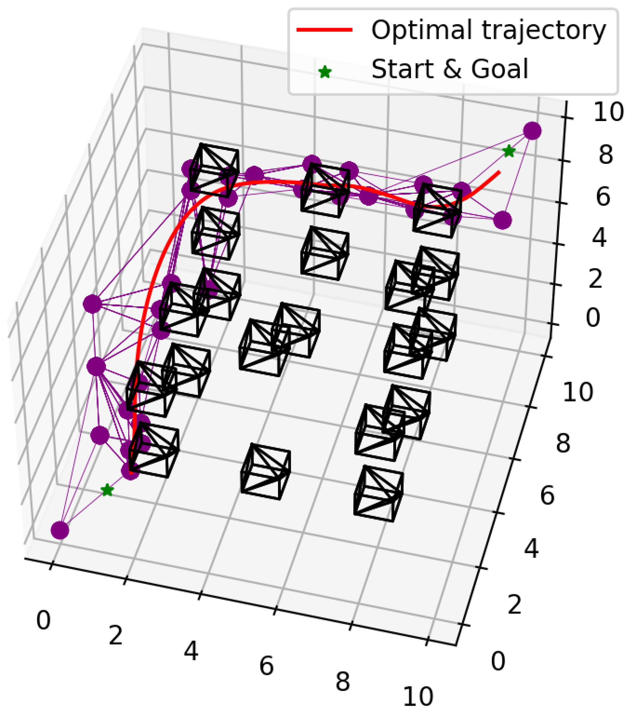
Figure 1.
Given a start and goal points in a 3D space that includes a random distribution of obstacles (black cuboids), our method generates a trajectory (red line) within a safe flight corridor represented as a sequence of tetrahedrons (purple edges and vertices).
The main contributions of this paper are as follows:
- We extend the concept of the dynamic map, initially introduced in [8], to effectively quantify uncertainty arising from dynamic environments;
- We propose a novel flight corridor generation method utilizing Delaunay triangulation and introduce a new trajectory optimization approach based on the generated flight corridor;
- The feasibility and effectiveness of the proposed method are evaluated through computer simulations, demonstrating that it can reduce the need for frequent replanning.
This paper is organized as follows. In Section 2, we review previous studies focusing on flight corridor generation and trajectory optimization. In Section 3, we outline the assumptions and preliminaries of our paper that clarify the foundational concepts and constraints of our study. In Section 4, we introduce the notion of 3D dynamic mapping and describe how it can be used to quantify the risk of collision. In Section 5, our method to generate a flight corridor for dynamic environments is described. Our B-spline-based method for trajectory optimization is presented in Section 6. In Section 7, we evaluate the proposed flight corridor generation method and the trajectory optimization method. Finally, in Section 8, we present our conclusions and future lines of work.
2. Related Work
Trajectory planning is the process of creating an optimal, feasible, and collision-free trajectory connecting two given UAV states describing the position, orientation, and dynamical features of the UAV under consideration. The largest accessible space for the UAV is known as the safe flight corridor. A safe flight corridor can be formulated as a set of safety constraints that are imposed during trajectory optimization, along with other UAV dynamical constraints. In this section, we first discuss previous work on flight corridor generation and review existing proposals on trajectory optimization.
Previous studies on flight corridor generation have sought to identify safe regions in the space, i.e., regions that are not occupied by static obstacles. To identify safety regions, the authors of [9] proposed a method consisting of growing an ellipsoidal region around a given location on a map until an obstacle is reached. The authors of [10] extended the strategy proposed by [9], using an initial path in the space as a sequence of segments and growing free ellipsoidal regions around each line segment. However, expanding the ellipsoidal regions is an iterative process, which is time-consuming and computationally demanding. To reduce the time and computational burden of this process, the authors of [11] proposed a method that expands each sampled location from an initial path to form the largest accessible free space, and similarly, the authors of [12] designed a method that inflates each sample into a spherical space.
Trajectory optimization methods can be grouped into two families, namely discrete-time and continuous-time methods. Discrete-time methods [13,14,15] represent the trajectory as a sequence of waypoints. The location of each waypoint is optimized using the gradient of a field representing the distance to the closest obstacle, resulting in waypoints being pushed away from the obstacles. The quality of the trajectory depends on the number of waypoints used, which has to be set before trajectory optimization and cannot therefore be modified during optimization.
Continuous-time methods use basis functions to define the trajectory as a function of time. The most common basis functions include monomial, Bernstein, and B-spline functions. References [11,16,17] formulated a quadratic programming problem with the coefficients of the piecewise monomial functions as the decision variable. However, the solution to this quadratic problem involves matrix inversion, which may cause numerical instability. As an extension to this formulation, the authors of [18] reformulated the problem by using endpoint derivatives as the decision variable to find an analytical solution. One of the drawbacks of this method is that it does not include a collision cost when optimizing the trajectory. To alleviate this, refs. [19,20] incorporated the collision cost into the penalty function. This introduces a new challenge, as the inclusion of the collision cost results in a non-convex problem, which can lead to failures in finding the optimal solution.
Other curves to represent trajectories have also been explored; for example, piecewise Bezier curves [21], as well as a variety of B-splines, including quintic uniform B-splines [7], clamped uniform B-splines [5], and non-uniform B-splines [22]. In [22], non-uniform B-splines are used to represent the trajectory, and non-uniformly distributed knots are utilized to optimize the time of the trajectory. Compared to the coefficients of monomial functions, the use of control points as decision variables makes the optimization process less prone to numerical instabilities. In addition, both Bezier curves and B-splines are characterized by the strong convex hull property, and consequently, the resulting trajectory is always inside the convex region defined by the control points, which guarantees the safety of the trajectory. Furthermore, B-splines have local support; therefore, changing the control points only influences a section of the generated trajectory, making it adaptable to dynamic environments. In this work, we use clamped B-splines as basis functions, since B-splines offer the desirable properties of a convex hull and local support. Our calculated flight corridor can be directly used as control points to construct a flight trajectory.
3. Assumptions and Preliminaries
A typical UAV navigation system consists of four main modules: sensing/perception, mapping, planning, and controlling. The approach presented in this paper addresses the challenges presented by unknown and dynamic environments during UAV trajectory planning. Hence, for the purpose of this study, we assume that a map describing the environment is available for planning. Specifically, we assume that the mapping module provides a map of the environment that:
- Detects the shapes and orientations of the obstacles and represents them using bounding boxes;
- Detects the velocities of dynamic obstacles and therefore distinguishes between static and dynamic obstacles.
Furthermore, the embedded bounding boxes are expanded by incorporating the radius of the UAV. This allows us to treat the UAV as a point on the map for trajectory planning purposes.
We divide the problem of trajectory planning into three key tasks:
- Dynamic map generation, which allows us to represent the uncertainty caused by dynamic obstacles;
- Flight corridor generation, after which an initial path and the largest free space around the path are created;
- Trajectory optimization, which provides a final trajectory guaranteeing dynamic feasibility and safety.
Each task is described in detail in the subsequent sections.
4. Dynamics Modeling and Collision Checking
Dynamic environments consist of both static and dynamic obstacles, i.e., obstacles whose states remain the same and obstacles whose states change over time. To include the uncertainty caused by the movements of dynamic obstacles, we extend our previous work [8] and develop a three-dimensional dynamic map to quantify the risk of future collisions between the UAV and the static/moving obstacles.
4.1. Dynamic Map Representation
We use the notion of a dynamic map proposed in [8] to represent a dynamic environment. A dynamic map is created by expanding the space occupied by obstacles according to their current state and their predicted future movements, which is estimated using Kalman filter approaches.
The state of the i-th obstacle is defined as follows:
where k denotes time, is the center of the i-th obstacle, and is its velocity. Using , we can produce an a priori prediction of the state of the obstacle after h time steps, which we denote as follows:
where and are the estimations of the center and velocity of the obstacle at time based on the known state .
The dynamic map corresponds to the probability that the center of the i-th obstacle will reach position after h time steps, given perfect knowledge of the current state [8]. To build a dynamic map, the predicted position together with an estimation of its uncertainty are needed. Both values are supplied by a prediction algorithm, e.g., the state covariance matrix in Kalman approaches.
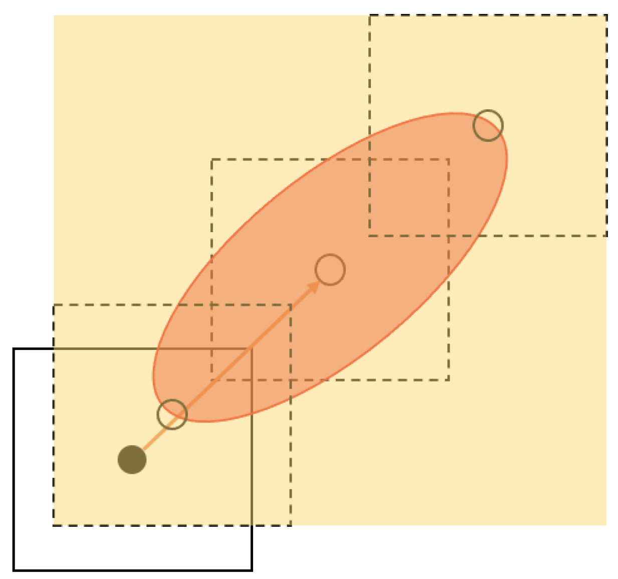
Using the dynamic map, a potential collision region can be obtained as the convolution of the bounding box representing the obstacle and the region where the dynamic map is greater than a predefined threshold , (see Figure 2). We then define the expanded obstacle at time instant as the smallest bounding box covering the potential collision region associated with obstacle i. In the case of static obstacles, coincides with the obstacle itself. Our collision detection method described in Section 4.2 will check the collisions between the current trajectory and each extended obstacle for each horizon value h.
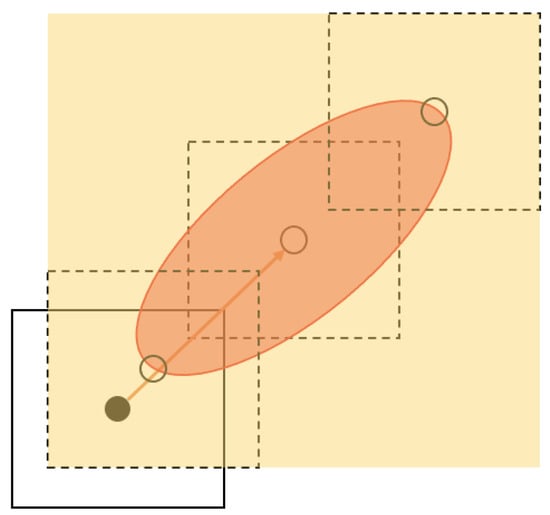
Figure 2.
Expanded obstacle (yellow region). The solid square represents an obstacle i at time instant k. Its center is represented as a solid dot. The arrow represents the estimation of movement of the obstacle, as given by, e.g., a Kalman filter approach. The orange ellipse corresponds to the locations where . Dashed squares represent the obstacle after h time instants in potential locations indicated by empty dots. Convolving the region where and the bounding box describing the obstacle, a potential collision region is obtained. The expanded obstacle is obtained as the smallest bounding box covering the potential collision region.
4.2. Collision Detection
Our collision detection method is based on the Möller–Trumbore intersection algorithm [23], which finds the intersection point between a ray and a plane. Given a segment of a trajectory and an axis-aligned bounding box representing an obstacle, our method proceeds by first extending the segment into a ray and each face of the bounding box into a plane. Then, it looks for the points where the ray intersects each plane. This method establishes that there is a collision if any intersection point belongs to the original segment and obstacle faces.
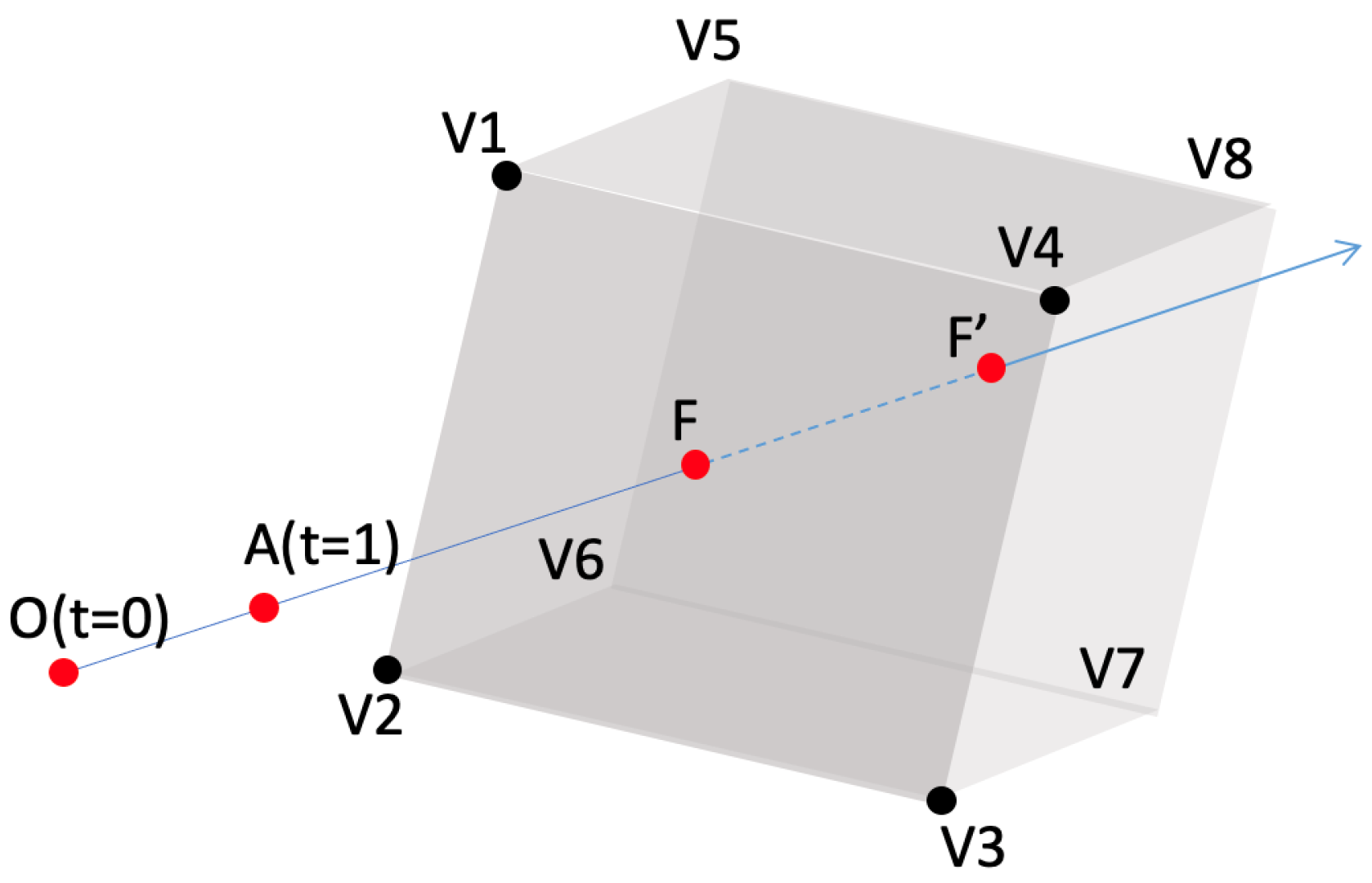
Let , , , and be four vertices defining one of the faces of the bounding box representing a given obstacle, let be the normal vector of the plane containing this face, and let be a trajectory segment defined by points and (Figure 3). A ray starting from point and going through can be represented as the following parametric equation:
where t is the parameter of the ray and defines the direction of the ray. Note that the starting point of the segment can be obtained as , the end point is , and any point within the original segment can be formulated as , where .
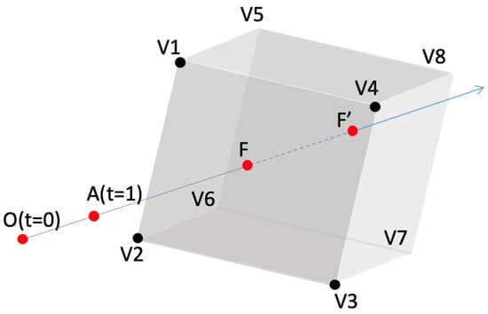
Figure 3.
An illustration of the implementation of the Möller–Trumbore ray-triangle intersection algorithm for collision detection. The ray, shown as a blue arrow line, intersects with the face --- at point F and the face --- at point . Since points F and ’s intersection times are not within the interval , the segment does not collide with the bounding box.
If an intersection point between the plane defined by , , , and and the ray exists, then the following equations are satisfied:
Solving for , we obtain the following:
Note that whenever , the ray is parallel to the plane. Once the value is found, we will decide that the segment intersects the face if
- , i.e., the intersection point lies within the original segment,
- the intersection point lies inside the face defined by vertices ---.
To check the second condition, we solve two sub-problems, namely whether the point lies inside triangle -- or triangle --. Consider the problem of determining whether belongs to triangle --. By extending one of the edges of triangle -- (for instance, ), we can split the plane defined by the triangle into two semi-planes, such that the remaining vertex () lies on one of the semi-planes. We can then check if belongs to the same semi-plane as the remaining vertex. Intersection point is inside the triangle if and only if it lies on the same semi-plane as the remaining vertex for the three splits defined by , , and . This condition is true if the following inequalities hold:
If an intersection point is identified, the method will establish that there is a collision and will trigger the replanning method.
5. Uncertainty-Aware Flight Corridor Generation
As described in Section 4, we represent dynamic environments using a dynamic map, where static and dynamic collision regions are modeled as bounding boxes. In this section, we describe how a dynamic map can be used to generate a flight corridor in dynamic environments.
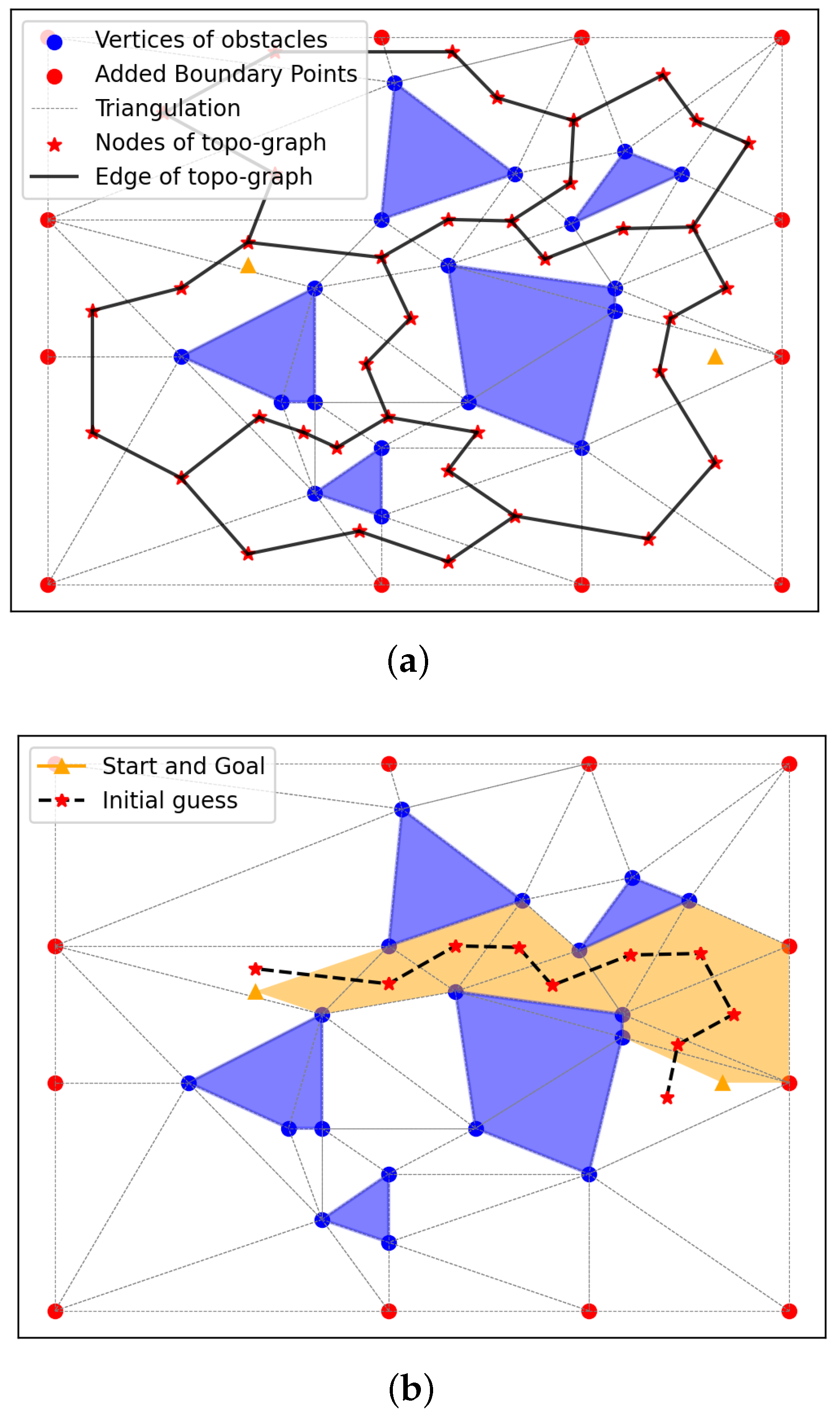
Our flight corridor generation method is inspired by [24], where collision-free segments connecting vertices of obstacles are created, and [25], where Delaunay triangulation is used to divide the space into non-overlapping partitions, i.e., triangles in 2D and tetrahedrons in 3D. Using the space partitioning obtained via Delaunay triangulation, the proposed method constructs a topo-graph , where node U represents the center of each collision-free partition and edge E represents the segment connecting the centers of neighboring free partitions. This topo-graph is a topological description of the free space and the basis for finding a path that defines a flight corridor as the union of the partitions corresponding to each one of the nodes that make up the path (Figure 4).
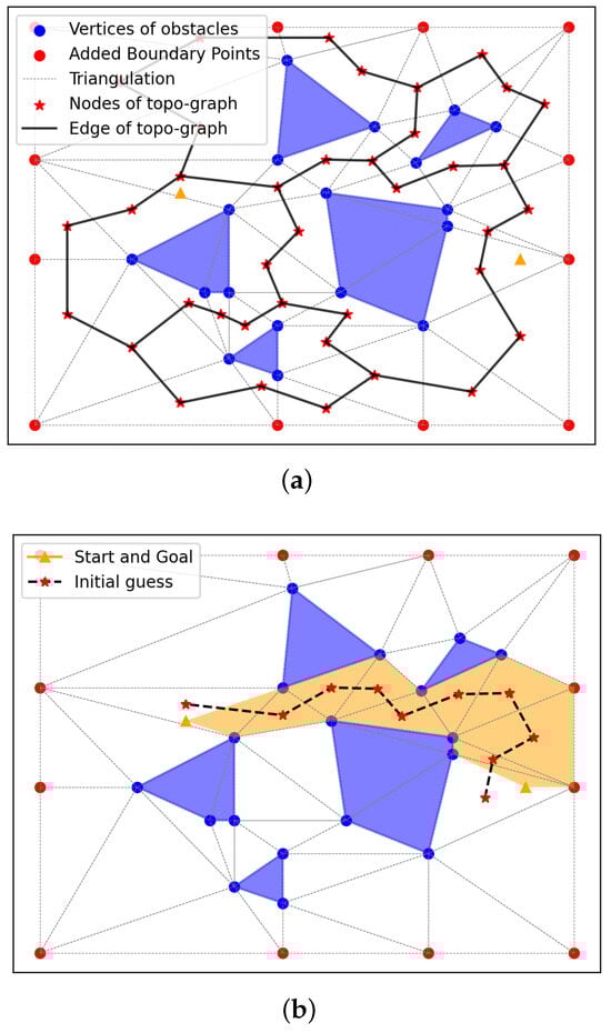
Figure 4.
An example of the generated flight corridor in 2D. In Panel (a), the blue polygons are the obstacles, the blue dots are the obstacle vertices, and the red dots are the virtual vertices, which are sampled from the boundary of the detection range described in Section 5.1. The constructed topo-graph nodes are marked as red stars, and edges are black solid lines. In Panel (b), the triangles containing the start and goal are located, and by applying Dijkstra method to the constructed topo-graph, the initial path is obtained (red stars and black dashed lines). The triangles that the path goes through constitute the flight corridor (shaded in orange).
5.1. Space Partition
The space is partitioned into non-overlapping regions using Delaunay triangulation on the vertices defining the obstacles and the detection boundary. The latter are referred to as virtual vertices. Virtual vertices allow us to explore the free space adequately and deal with scenarios where there are few obstacles.
5.2. Graph Construction
The centers of all the partitions obtained using Delaunay triangulation are calculated and stored as nodes U of the topo-graph G. The edges E are obtained as the segments linking neighboring partitions.
5.3. Edge Cost
A cost is assigned to each edge in the graph. This cost accounts for the length of the edge, i.e., the euclidean distance between adjacent graph nodes, and a collision cost, which is a constant value added to the edge cost whenever an extended obstacle overlaps one of the partitions that the edge goes through.
5.4. Initial Path and Flight Corridor
An initial path linking the starting and destination points is created by applying the Dijkstra algorithm to the graph G using the edge cost previously defined. This path consists of a sequence of graph nodes and implicitly defines a flight corridor as the union of the partitions whose centers are the nodes defining the path.
6. Uniform Clamped B-SPLINE Trajectory Optimization with Time Allocation
In this section, we describe our method to generate trajectories using B-splines. Thanks to the properties of local support and a convex hull, using a B-spline representation guarantees the safety of the generated trajectories. In addition, B-splines are fast to compute and adaptable to dynamic environments where trajectory modifications might be needed.
6.1. Trajectory Representation
A B-spline function is defined by control points , where , and knots such that , where Q is the order of the B-spline. According to the property of local support, each trajectory segment is defined by control points. In our case, as free space is partitioned into tetrahedrons, segments are defined by four control points and hence the order of the function is set to . In this paper, we implement a uniform clamped B-spline function, where the first and last knots have multiplicity of to ensure the B-spline function goes through the start and goal points, and knots are uniformly distributed within the range of .
Our B-spline function is defined as follows:
where , is the B-spline function, calculated using the Cox–de Boor recursion formula given the order Q and the set of knots, and is the coordinate of the ith control point.
The velocity along the generated curve is the first derivative of , denoted by . Accordingly, it can be regarded as a B-spline curve of order on a new knot vector. The first and last knots have a multiplicity of Q with a new set of control points , where the new control points are obtained as follows:
By setting , Equation (8) can also be written in matrix form , where
and
Similarly, the acceleration is a B-spline curve of order with a set of control points , where
and , where
and
The same approach could be used to define other quantities such as the jerk, snap, and higher orders of derivatives of the generated trajectory.
6.2. Control Point Initialization
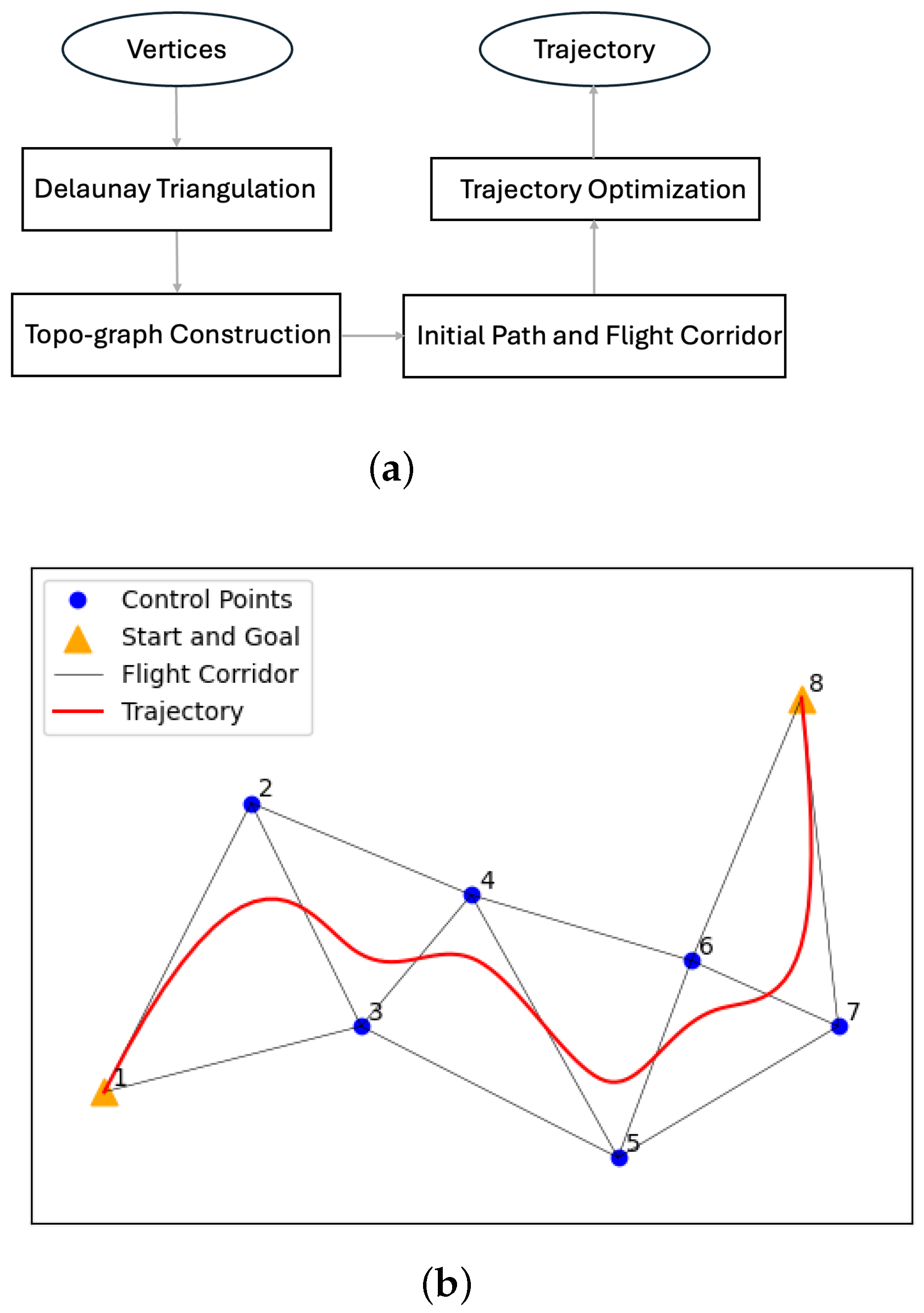
Figure 5b shows an 2D example of how the control points are found from the flight corridor, where the order of the B-spline function is 3. Similarly, the initial control points in 3D are the vertices of the tetrahedrons in the flight corridor. They are re-ordered to make sure that each segment of the trajectory is restrained within the partitions. The details about how to derive the control points are described in Algorithm 1.
| Algorithm 1 Find the control points for trajectory optimization |
|
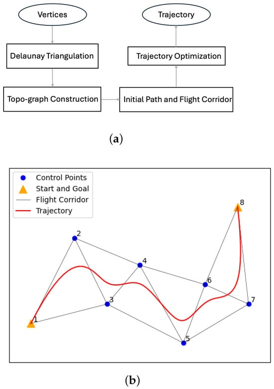
Figure 5.
The overall process of finding a flight corridor is summarized in (a) Flowchart of the proposed trajectory planning method described in Section 5 and Section 6. An example of the generated flight corridor is shown in (b) Example of a generated flight corridor and the corresponding control points used during trajectory optimization. Numbers represent the indices of the vertices. The first trajectory segment is computed using vertices 1, 2, 3, the second segment using 2, 3, 4, and so forth. Our flight corridor generation method consists of four steps that are subsequently described.
6.3. Trajectory Optimization
In this part, we formulate the optimization problem as a quadratic programming problem where the decision variables are the positions of the control points. The objective function and constraints defining the optimization problem are provided. Using vector notation, we can re-write Equation (7) as follows:
where subscript Q in is omitted for brevity. The B-spline functions for the velocity and acceleration and are defined in an analogous manner.
The first and second derivative of the trajectory can be expressed as follows:
and
In this paper, the objective J includes two penalties, , where is used to minimize the accelerations along the replanned trajectory. It can be obtained as follows:
where and is set as the decision variable.
Furthermore, the start and goal of the optimized trajectory are expected to be as close to the endpoints of the original trajectory as possible so that the current state connects to the replanned trajectory smoothly. Thus, we add another penalty into the objective, defined as follows:
where is a vector that includes the positions of the original start and goal, and S is the permutation matrix, defined as follows:
The construction of is omitted for brevity. The weight for the second part of the objective is to balance the numerical difference between and .
Additional constraints must be applied in order to ensure the smoothness between the current state and the replanned trajectory, and to ensure that the optimized control points are within the flight corridor.
6.3.1. Endpoint Constraints
The equality constraints on the velocity of the start and end of the trajectory are expressed as follows:
Currently, we assume that the velocities of the start and goal are . The reason we do not impose inequality constraints on the other velocities along the trajectory is that parameter t for B-spline function is within , and every time a trajectory is optimized, we re-allocate the time for each sample on the trajectory, as explained in Section 6.4, to make sure that the constraint on the maximum velocity is satisfied.
6.3.2. Safety Constraints
As discussed in Section 6.2, each trajectory segment is calculated using four adjacent control points corresponding to a tetrahedron that represents the largest free space. To ensure the safety of each segment, the optimized control points must remain within the corresponding tetrahedron, guaranteeing that the entire segment lies entirely within the free space.
Suppose that the four tetrahedron’s vertices are , , , and . A random point K lies on the same side of plane as the opposite vertex of the tetrahedron when the following constraint is satisfied:
where is the normal vectors of plane . We can reformulate (21) as follows:
where and are the coordinates of points and , respectively.
Point K is inside the tetrahedron if it satisfies the same-side condition for the other three planes, , , and . We can formulate the other three constraints using an expression analogous to (22) and combine them in matrix form as follows:
where , , and are the normal vectors of planes , , and . Thus, the safety of the optimized trajectory is ensured by constraining each control point in the corresponding tetrahedron by formulating the constraint as (23).
6.4. Time Allocation
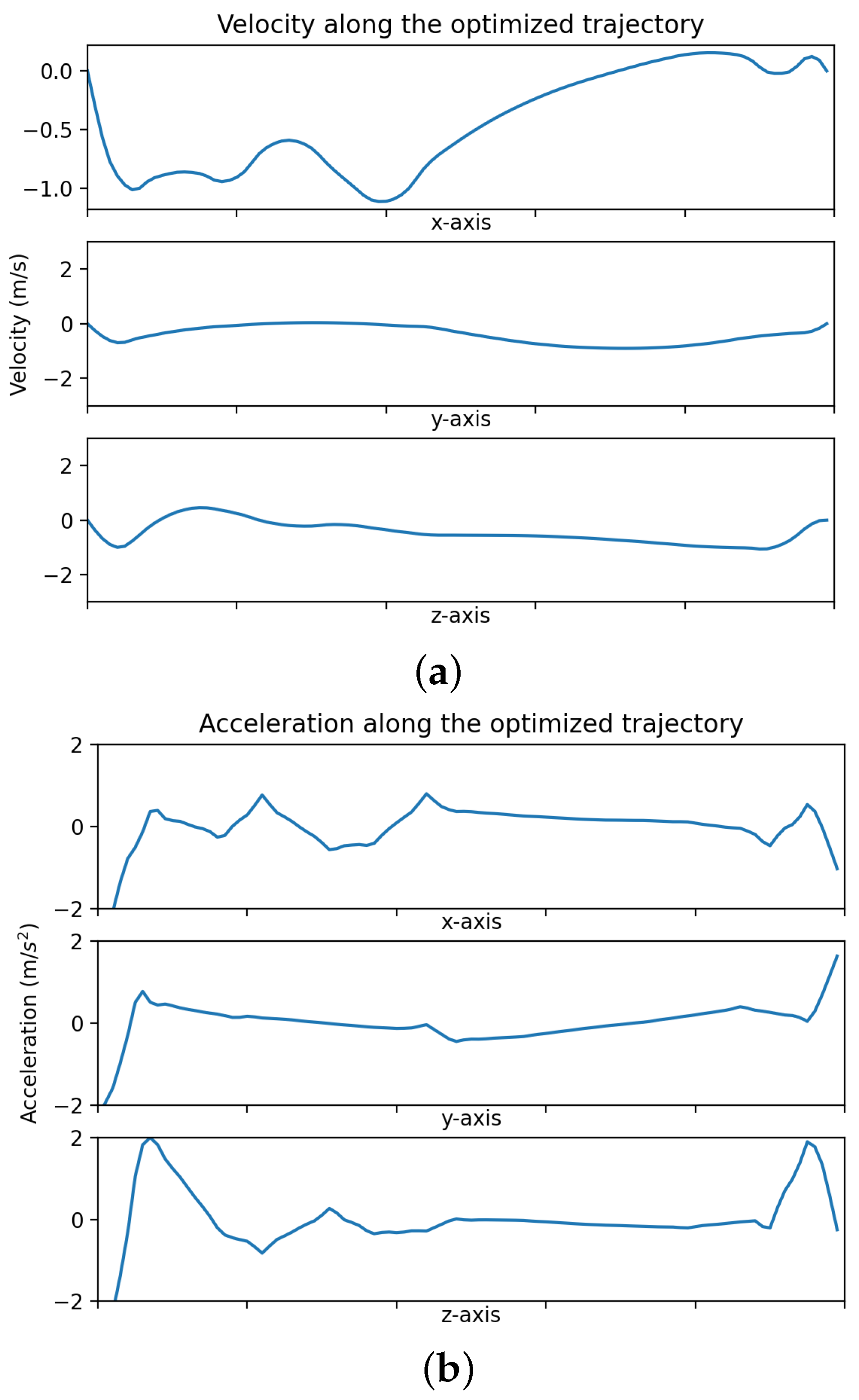
Suppose that the maximum velocity and acceleration are and , respectively, and the largest acceleration and the largest velocity along the trajectory are and . Then, the total time can be calculated as follows in Equation (24) and Figure 6:
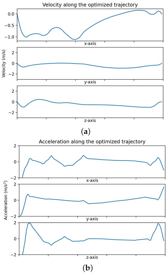
Figure 6.
The performance of an generated trajectory from the start to the goal position with fixed velocity : the maximum velocity and acceleration for each axis is 3 m/s and 2 m/s2.
6.5. Intermediate/Local Goal Selection
When a replanned trajectory is needed, the start point of the local map will be the current position, and the goal will be selected from the future global trajectory. We will search the unfulfilled global trajectory to find a collision-free point according to the current local map and set it as the local goal.
7. Experiments
In this section, we show the validations of the two proposed algorithms, namely the flight corridor generation algorithm in Section 5 and the trajectory optimization algorithm in Section 6.
7.1. Simulation Implementation Details
The simulations for the flight corridor generation and trajectory optimization are implemented in Python, and the quadratic programming problem in Equation (17) is solved using the software package CVXOPT [26].
To simulate a scenario that is as real as possible, we construct a 3D space of 11 m × 11 m × 12 m using the 10 m maximum detection range of Intel®RealSenseTM D435 [27] as a reference. The obstacles are cuboids of size 1 m × 1 m × 1 m, and they can be static or dynamic, with a speed randomly picked from six possible velocities, including , , , , , and . The initial trajectory for the UAV is a straight line from the start position to the goal position , and when the proposed method is tested in dynamic environments, the moving obstacles are intentionally designed to collide with the initial trajectory.
For the trajectory generation, we set the order Q of the B-spline function as 3 so that the generated trajectory stays inside the region enclosed by any four consecutive control points. The maximum velocity is set to 3 m/s, and the maximum acceleration is 2 m/s2.
7.2. System Evaluation
In Section 4, we introduced the concept of a dynamic map to quantify the uncertainty caused by dynamic environments. We evaluate its effectiveness based on the number of replanning events triggered by obstacles moving in the environment. The flight corridor generation method in Section 5 is evaluated by measuring the processing time required to create a safe flight corridor under varying obstacle densities. The performance of the trajectory optimization method in Section 6 is assessed in terms of processing time and the quality of the optimized trajectory, focusing on two key aspects: time optimality and safety. Time optimality is assessed using the total trajectory duration and length, while safety is measured based on the minimum distance between the trajectory and the surrounding obstacles. These properties are compared across a range of scenarios involving different obstacle densities and a mix of static and dynamic obstacles.
7.3. Results
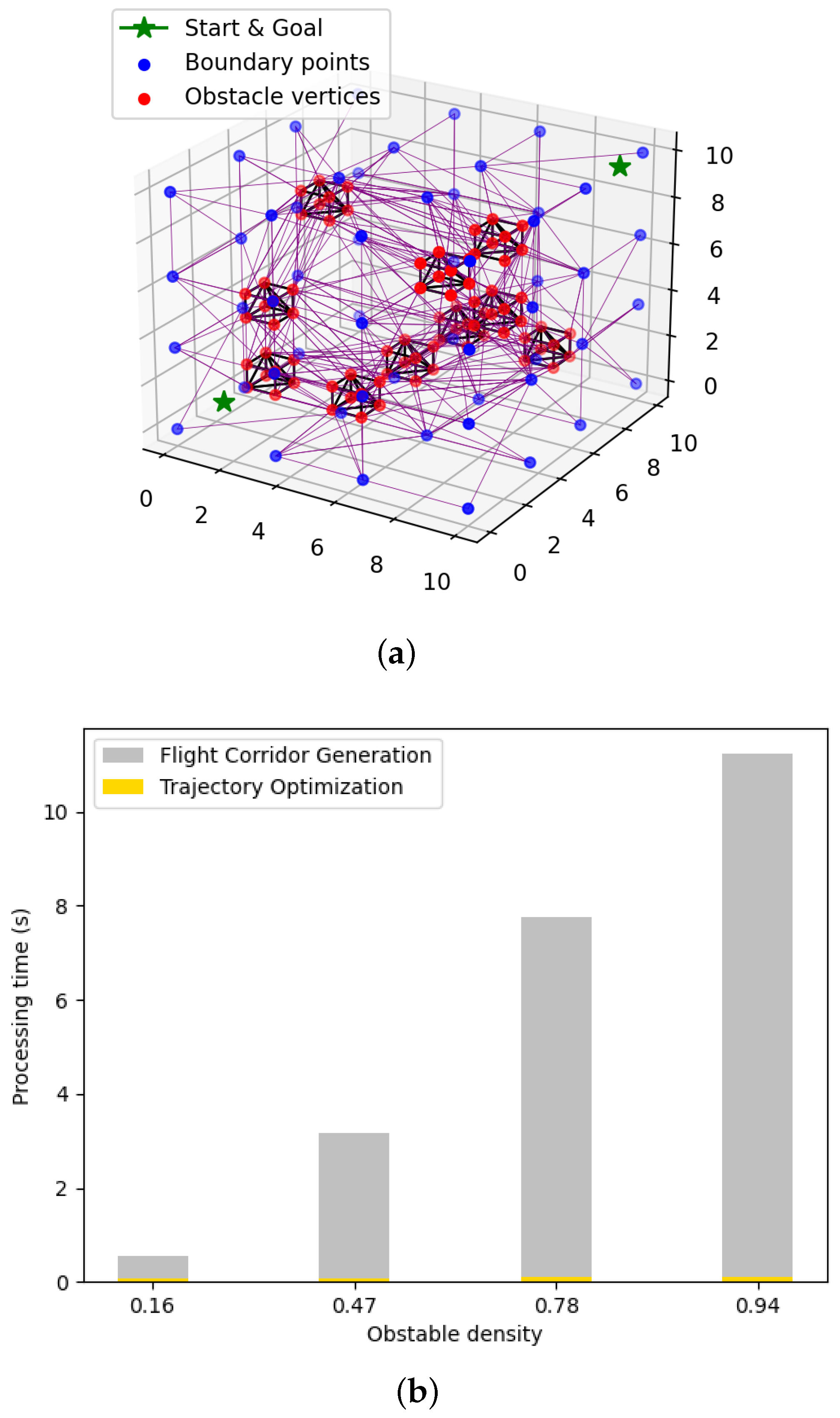
Figure 7b shows the relationship between processing time and obstacle density, which is calculated as the number of obstacles divided by the maximum number of obstacles this space can accommodate. As shown in Figure 7b, the flight corridor generation method takes several seconds, while the trajectory optimization method only needs a few milliseconds.
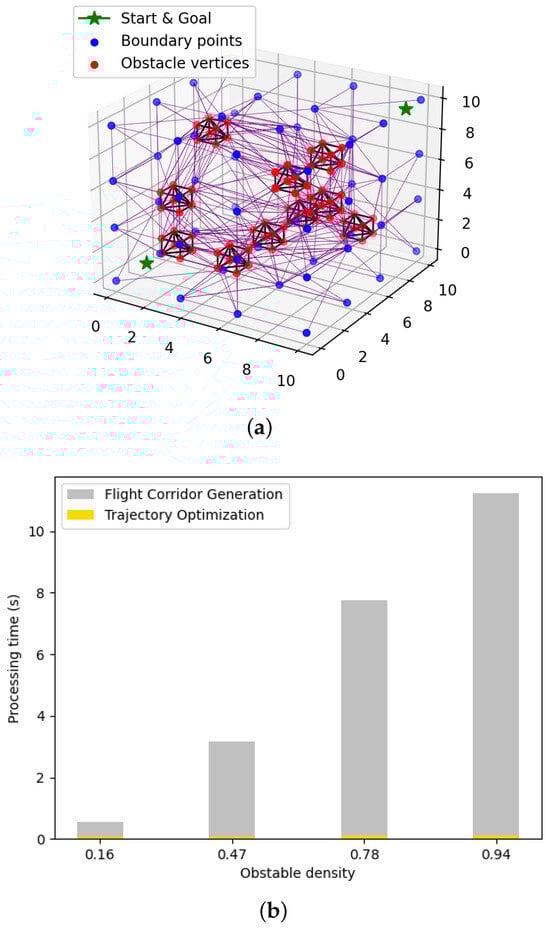
Figure 7.
(a) Constructed flight corridor. The blue dots are the added virtual vertices. The red dots together with the black solid lines represent the obstacles. The partitions of the free space using Delaunay triangulation are shown with purple solid lines. (b) Comparison between the processing time of the flight corridor generation method (in grey) and trajectory optimization method (in yellow) under different obstacle densities.
7.3.1. Flight Corridor Generation
Figure 7a illustrates the process of constructing a flight corridor where the free space is partitioned into tetrahedrons using Delaunay triangulation. Figure 7b, shows that the time used to calculate the flight corridor increases exponentially as the number of vertices grows, which would be realistic for a real-world scenario.
7.3.2. Trajectory Optimization
In Table 1, a comparison between the trajectory generated by the optimized control points and the initial control points is illustrated. It shows that the optimized trajectory has a higher average velocity with a smaller length and shorter time. Furthermore, the velocities and accelerations along a generated trajectory from to with given velocity (the simulated UAV is initially still) are illustrated in Figure 6a,b. It can be observed that the velocity and acceleration are constrained within their maximum values m/s and m/s2 and change smoothly.

Table 1.
A simple comparison between the original trajectory, calculated based on the initial control points and the optimized trajectory.
In Table 2, we evaluate the performance of the proposed method in static environments under different obstacle densities and in dynamic environments when there are static and moving obstacles simultaneously. We also implement our proposed method without utilizing the uncertainty information when optimizing the trajectories and compare with the cases when we consider the uncertainty.
Table 2.
The evaluation of the optimized trajectory using the proposed method. The “Uncertainty-unaware dynamic” section demonstrates the performance of our proposed method when applied in a dynamic environment, excluding considerations for the motion of dynamic obstacles.
Static environments: In Table 2, under the first entries ‘Prop.static’, there is a steep drop in the performances of the replanned trajectory due to the increasing number of obstacles. With more obstacles, the gaps between obstacles become narrower, resulting in the windings of the trajectories, slowing down the UAV.
Dynamic environments: By comparing the second entry ‘Prop.dynamic’ and ‘without dyn.dyn’, we can easily observe that introducing the uncertainty caused by moving obstacles can help to reduce the times of replanning, which proves the feasibility of our proposed method in a dynamic environment.
8. Conclusions and Future Work
In this paper, we propose a different strategy to model dynamic environments and optimize the trajectories using an uncertainty-aware fashion. First, we implement a Delaunay triangulation-based space partition method to construct the safe flight corridor and find the corresponding topological description of the environments, the topo-graph. Then, we introduce the uncertainty information into the topo-graph using the notion of the dynamic map, as proposed in our previous work [8]. Finally, a B-spline-based trajectory is generated from the path found in the topo-graph and using the safe flight corridor as a constraint.
Our simulations indicate that this strategy accomplishes the above tasks and successfully reduces the times of replanning by introducing uncertainty information caused by moving obstacles into trajectory optimization. The proposed approach can be further improved in different ways. First of all, the complexity associated with constructing a safe flight corridor in 3D space is , and the simulation results show that it can take up to several seconds to process, which would be a limiting feature in real-world scenarios. Secondly, we implement the Dijkstra algorithm to find the path, which is considered time-consuming. In the future, we plan to use other heuristic graph search algorithms for comparisons and efficiency improvements. Apart from that, when optimizing, assigning more time to a specific time span, which violates the constraints of maximum velocity/acceleration, instead of assigning more time to the whole trajectory, also helps to improve efficiency. To overcome this bottleneck, a promising avenue is to find an incremental way to update the newly found obstacles in the constructed space partition and allocate time to the segments of the whole trajectory separately according to their corresponding violations of velocity/acceleration. Finally, to further validate our method, we plan to integrate our trajectory planning approach with a mapping module that satisfies our assumptions, forming a coupled system. This integration will enable more comparisons with state-of-the-art methods and validations in real-world scenarios.
Author Contributions
Conceptualization, J.M.; methodology, J.M.; software, J.M.; validation, J.M.; formal analysis, J.M.; investigation, J.M.; resources, J.M.; data curation, J.M.; writing—original draft, J.M.; writing—review and editing, J.M. and J.R.C.; visualization, J.M.; supervision, J.R.C. All authors have read and agreed to the published version of the manuscript.
Funding
This research received no external funding.
Data Availability Statement
The data presented in this study are available upon request from the corresponding author due to privacy.
Conflicts of Interest
The authors declare no conflicts of interest.
References
- Tsouros, D.C.; Bibi, S.; Sarigiannidis, P.G. A review on UAV-based applications for precision agriculture. Information 2019, 10, 349. [Google Scholar] [CrossRef]
- She, R.; Ouyang, Y. Efficiency of UAV-based last-mile delivery under congestion in low-altitude air. Transp. Res. Part C Emerg. Technol. 2021, 122, 102878. [Google Scholar] [CrossRef]
- Tordesillas, J.; Lopez, B.T.; How, J.P. FASTER: Fast and Safe Trajectory Planner for Flights in Unknown Environments. In Proceedings of the IEEE International Conference on Intelligent Robots and Systems, Macao, 3–8 November 2019; Institute of Electrical and Electronics Engineers Inc.: Piscataway, NJ, USA, 2019; pp. 1934–1940. [Google Scholar] [CrossRef]
- Zinage, V.; Arul, S.H.; Manocha, D. 3D-OGSE: Online Smooth Trajectory Generation for Quadrotors using Generalized Shape Expansion in Unknown 3D Environments. In Proceedings of the IEEE International Conference on Robotics and Automation, Singapore, 20–22 November 2020. [Google Scholar] [CrossRef]
- Tordesillas, J.; How, J.P. MADER: Trajectory Planner in Multiagent and Dynamic Environments. IEEE Trans. Robot. 2022, 38, 463–476. [Google Scholar] [CrossRef]
- Ingersoll, B.; Ingersoll, K.; Defranco, P.; Ning, A. UAV path-planning using bézier curves and a receding horizon approach. In Proceedings of the AIAA Modeling and Simulation Technologies Conference, Washington, DC, USA, 13–17 June 2016; American Institute of Aeronautics and Astronautics Inc. AIAA: Reston, VA, USA, 2016. [Google Scholar] [CrossRef]
- Usenko, V.; Stumberg, L.V.; Pangercic, A.; Cremers, D. Real-Time Trajectory Replanning for MAVs using Uniform B-splines and a 3D Circular Buffer. In Proceedings of the IEEE International Conference on Intelligent Robots and Systems, Vancouver, BC, Canada, 24–28 September 2017; pp. 215–222. [Google Scholar]
- Men, J.; Requena Carrion, J. A Generalization of the CHOMP Algorithm for UAV Collision-Free Trajectory Generation in Unknown Dynamic Environments. In Proceedings of the 2020 IEEE International Symposium on Safety, Security, and Rescue Robotics, SSRR, Abu Dhabi, United Arab Emirates, 4–6 November 2020; Institute of Electrical and Electronics Engineers Inc.: Piscataway, NJ, USA, 2020; pp. 96–101. [Google Scholar] [CrossRef]
- Deits, R.; Tedrake, R. Computing large convex regions of obstacle-free space through semidefinite programming. In Proceedings of the Springer Tracts in Advanced Robotics; Springer: Berlin/Heidelberg, Germany, 2015; Volume 107, pp. 109–124. [Google Scholar] [CrossRef]
- Liu, S.; Watterson, M.; Mohta, K.; Sun, K.; Bhattacharya, S.; Taylor, C.J.; Kumar, V. Planning dynamically feasible trajectories for quadrotors using safe flight corridors in 3-D complex environments. IEEE Robot. Autom. Lett. 2017, 2, 1688–1695. [Google Scholar] [CrossRef]
- Chen, J.; Liu, T.; Shen, S. Online generation of collision-free trajectories for quadrotor flight in unknown cluttered environments. In Proceedings of the International Conference on Robotics and Automation, Stockholm, Sweden, 16–21 May 2016; Volume 2016, pp. 1476–1483. [Google Scholar] [CrossRef]
- Gao, F.; Shen, S. Online quadrotor trajectory generation and autonomous navigation on point cloud. In Proceedings of the 2016 IEEE International Symposium on Safety, Security, and Rescue Robotics, SSRR, Lausanne, Switzerland, 23–27 October 2016. [Google Scholar]
- Nathan, R.; Zucker, M.; Bagnell, J.; Srinivasa, S. CHOMP: Gradient Optimization Techniques for Efficient Motion Plan. In Proceedings of the International Conference on Robotics and Automation, Kobe, Japan, 12–17 May 2009; p. 9. [Google Scholar]
- Dragan, A.D.; Ratliff, N.D.; Srinivasa, S.S. Manipulation planning with goal sets using constrained trajectory optimization. In Proceedings of the International Conference on Robotics and Automation, Shanghai, China, 9–13 May 2011; pp. 4582–4588. [Google Scholar] [CrossRef]
- Zucker, M.; Ratliff, N.; Dragan, A.D.; Pivtoraiko, M.; Klingensmith, M.; Dellin, C.M.; Bagnell, J.; Srinivasa, S.S. CHOMP: Covariant Hamiltonian Optimization for Motion Planning. Int. J. Robot. Res. 2013, 32, 1164–1193. [Google Scholar] [CrossRef]
- Mellinger, D.; Kumar, V. Minimum snap trajectory generation and control for quadrotors. In Proceedings of the International Conference on Robotics and Automation, Shanghai, China, 9–13 May 2011; pp. 2520–2525. [Google Scholar] [CrossRef]
- Mueller, M.W.; D’Andrea, R. A model predictive controller for quadrocopter state interception. In Proceedings of the 2013 European Control Conference, ECC, Zurich, Switzerland, 17–19 July 2013; pp. 1383–1389. [Google Scholar] [CrossRef]
- Richter, C.; Bry, A.; Roy, N. Polynomial Trajectory Planning for Aggressive Quadrotor Flight in Dense Indoor Environments. In Robotics Research; Springer: Berlin/Heidelberg, Germany, 2016; pp. 649–666. [Google Scholar] [CrossRef]
- Oleynikova, H.; Burri, M.; Taylor, Z.; Nieto, J.; Siegwart, R.; Galceran, E. Continuous-Time Trajectory Optimization for Online UAV Replanning. In Proceedings of the IEEE International Conference on Intelligent Robots and Systems, Daejeon, Republic of Korea, 9–14 October 2016. [Google Scholar]
- Gao, F.; Lin, Y.; Shen, S. Gradient-based online safe trajectory generation for quadrotor flight in complex environments. In Proceedings of the IEEE International Conference on Intelligent Robots and Systems, Vancouver, BC, Canada, 24–28 September 2017; Volume 2017, pp. 3681–3688. [Google Scholar] [CrossRef]
- Gao, F.; Wu, W.; Lin, Y.; Shen, S. Online Safe Trajectory Generation for Quadrotors Using Fast Marching Method and Bernstein Basis Polynomial. In Proceedings of the International Conference on Robotics and Automation, Brisbane, Australia, 21–25 May 2018; pp. 344–351. [Google Scholar] [CrossRef]
- Zhou, B.; Gao, F.; Wang, L.; Liu, C.; Shen, S. Robust and Efficient Quadrotor Trajectory Generation for Fast Autonomous Flight. IEEE Robot. Autom. Lett. 2019, 4, 3529–3536. [Google Scholar] [CrossRef]
- Möller, T.; Trumbore, B. Fast, minimum storage ray/triangle intersection. In Proceedings of the Journal of Graphics Tools; Taylor & Francis Group: Oxford, UK, 1997; Volume 2, pp. 21–28. [Google Scholar] [CrossRef]
- Lozano-Pérez, T.; Wesley, M.A. An Algorithm for Planning Collision-Free Paths Among Polyhedral Obstacles. Commun. ACM 1979, 22, 560–570. [Google Scholar] [CrossRef]
- Bowyer, A. Computing dirichlet tessellations. Comput. J. 1981, 24, 162–166. [Google Scholar] [CrossRef]
- Andersen, M.; Dahl, J.; Vandenberghe, L. CVXOPT: Convex Optimization; University of Maryland: College Park, MD, USA, 2020. [Google Scholar]
- Intel. Intel® RealSense™ Depth and Tracking Cameras D435. 2024. Available online: https://www.intelrealsense.com/depth-camera-d435/ (accessed on 10 October 2024).
Disclaimer/Publisher’s Note: The statements, opinions and data contained in all publications are solely those of the individual author(s) and contributor(s) and not of MDPI and/or the editor(s). MDPI and/or the editor(s) disclaim responsibility for any injury to people or property resulting from any ideas, methods, instructions or products referred to in the content. |
© 2024 by the authors. Licensee MDPI, Basel, Switzerland. This article is an open access article distributed under the terms and conditions of the Creative Commons Attribution (CC BY) license (https://creativecommons.org/licenses/by/4.0/).