Abstract
This paper proposes a hybrid position–force control strategy for overconstrained cable-driven parallel robots (CDPRs). Overconstrained CDPRs have more cables (m) than degrees of freedom (n), and the idea of the proposed controller is to control n cables in length and the other ones in force. Two controller implementations are developed, one using the motor torque and one using the motor following-error in the feedback loop for cable force control. A friction model of the robot kinematic chain is introduced to improve the accuracy of the cable force estimation. Compared to similar approaches available in the literature, the novelty of the proposed control strategy is that it does not rely on force sensors, which reduces the hardware complexity and cost. The developed control scheme is compared to classical methods that exploit force sensors and to a pure inverse kinematic controller. The experimental results show that the new controller provides good tracking of the desired cable forces, maintaining them within the given bounds. The positioning accuracy and repeatability are similar those obtained with the other controllers. The new approach also allows an online switch between position and force control of cables.
1. Introduction
Cable-driven parallel robots (CDPRs) are parallel manipulators in which cables replace rigid links for the actuation of the end-effector [1]. Using cables guarantees a larger workspace and fewer moving masses compared to other robots, allowing CDPRs to achieve high dynamic performances even in wide areas. In most cases, the actuation system comprises a motor (with or without a gearbox) connected to a drum on which the cable is coiled [2]. After exiting each drum, the cable often engages a set of transmission pulleys before arriving at the end-effector. Pulleys are also an ideal place to install the force sensors (usually load cells) necessary to measure the force acting on each cable.
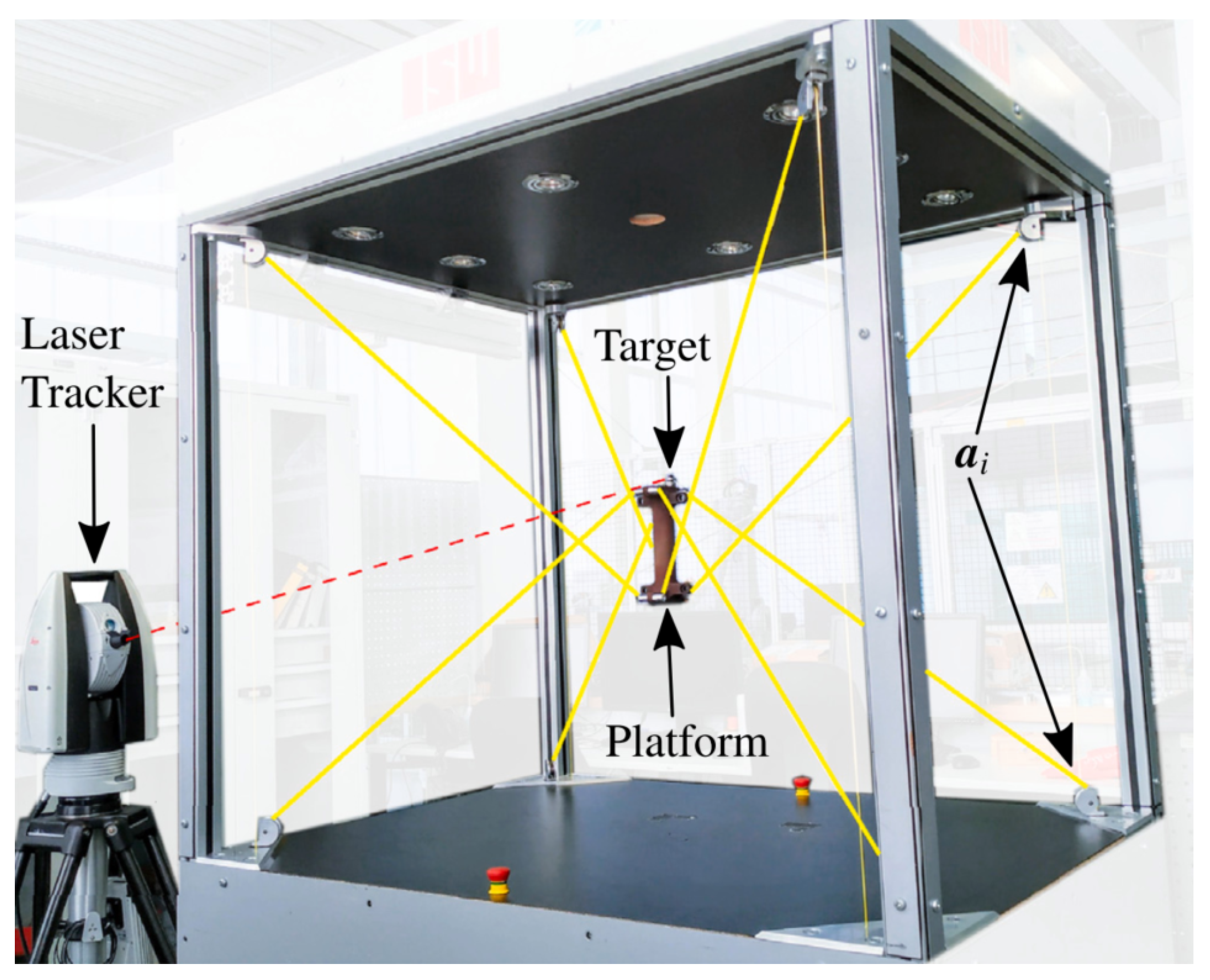
The main disadvantage of CDPRs is that cables can only exert tensile forces. For this reason, to fully control a robot with n degrees of freedom (DOFs) it is necessary to use at least actuated cables, which makes the robot overconstrained. The degree of redundancy is . In spatial applications requiring six DOFs, it is common to use CDPRs with eight cables, as in the case of the IPAnema family [3]. One of these robots, the IPAnema 3 Mini (Figure 1), is used to test the control technique proposed in this paper. More information about the geometry of the IPAnema 3 Mini can be found in [4].

Figure 1.
IPAnema 3 Mini with the laser tracker used in the experiments. This picture is taken from [4].
During the last few years, many overconstrained CDPRs have been developed for different aims: in the logistics field for warehousing applications [5,6,7,8], for the construction industry to build and maintain building facades [9,10], or in applications that require lifting heavy loads [11,12]. These robots are also helpful for rehabilitation tasks [13,14,15] or for window cleaning [16]. CDPRs with high dynamic capabilities [17,18] for classical 3-DOFs pick-and-place operations [19,20,21] or more complex bin-picking tasks [22] are particularly interesting.
Regardless of the application, one common issue for all overconstrained CDPRs is the suitable control of cable tensions. It is always desirable to have these in a predefined range, in such a way as to maintain the cables as permanently taut (i.e., with a tension higher than a lower limit) without damaging them (i.e., with a tension lower than a higher limit). To achieve this it is common to compute a theoretical force distribution for a given pose of the end-effector, and then apply a cascaded control to impose the computed tensions in the cables. The problem of finding a correct force distribution is not straightforward due to redundancy: different methods can be used for different purposes. Many algorithms are based on linear [23,24] or quadratic [25] programming optimization problems; however, the closed-form technique, first introduced in [26] and then expanded in [27,28], or geometric techniques [29,30,31,32] are the most interesting for real-time applications that require fast computations.
Once a force distribution is computed, forces must be converted into motor inputs, such as torques [33], velocities [34], or positions [32]. In general, in order to be sure to apply the desired tensions, the theoretical motor inputs must be modified by taking into account the real force values read by the force sensors [35]. When the end-effector must apply a specific wrench to an external object, a hybrid position–force control in Cartesian space may be applied. For this goal, the end-effector DOFs are divided according to their method of control, which is either in force or in position [36,37]. The same concept can be used in the joint space to develop a different hybrid position–force control. We will refer to this method as hybrid joint-space control (HC). This concept was first introduced in [38,39]: the idea is to control the lengths of n cables of the robot to obtain a specific pose of the end-effector and to perform a force control on the r redundant cables to obtain the desired force distribution. Mattioni et al., in [40,41], further developed this idea by introducing a method (based on the force distribution sensitivity index) that allows the r force-controlled cables to be chosen among the overall m wires.
The present paper aims to extend the HC by presenting, for the first time, a strategy to apply it without using any force sensor. The possibility of implementing a control scheme that allows cable tensions to be maintained within given bounds without force sensors decreases hardware complexity and cost. To achieve this, a friction model to estimate the actual cable force from the motor torque is introduced in the control feedback loop. This model is used in both the approaches that we will present in the following: one based on the motor-torque reading (HC-), the other based on the following-error feedback (HC-e). In particular, the HC-e method is, to the authors’ knowledge, unexplored at the moment. Another notable result of the paper is to prove that force- and length-controlled cables can be switched in real-time, which increases the workspace in which the robot can operate with satisfactory performance.
Both controllers HC- and HC-e will be compared with other state-of-the-art techniques, such as:
- the classical approach that exploits force sensors (HC-f), as applied in [38,39,40];
- the nullspace control strategy (NC) proposed in [4,42], which exploits load cells to maintain cable forces always positive without computing a force distribution;
- a pure inverse kinematic controller (IKC), which (as the new controllers proposed in this paper) does not use force sensors, but it does not involve any correction to maintain cable tensions within predefined bounds.
The comparison will be performed by analyzing the effect of the controller on the real cable forces, as well as the accuracy and repeatability of the manipulator.
The controllers HC- and HC-e can be applied to all overconstrained CDPRs. However, in this paper, they are mainly developed for light robots capable of fast movements. In fact, the winches of these robots rotate at high velocities, making them particularly suitable for being directly driven by motors without the interposition of gear speed reducers. Avoiding gearboxes decreases friction in the kinematic chain, making the use of HC- and HC-e controllers easier. Moreover, the practical applications in which these robots are involved (e.g., for pick and place) commonly require continuous movements of the end-effector most of the time, so it is usually not necessary to exert static wrenches. For this reason, we will focus on modeling dynamic friction only, disregarding static friction. While complex models for friction in the kinematic chains of CDPRs are available in the literature [43,44], our work aims to test whether a simple model with few parameters can be used in the HC scheme to obtain satisfactory performance. The advantage of defining a friction model as simple as the one presented here is the possibility of making straightforward tests by only using hardware that is already mounted in the robot kinematic chain. In this way, tests can be repeated every time it is necessary, e.g., when some mechanical parts are re-designed or substituted due to wear.
The paper is organized as follows. Section 2 introduces the kinetostatic model of the IPAnema 3 Mini robot, the model of the dynamic friction in the kinematic chains, and the model to compute the motor following-error from its torque. Section 3 presents the force-sensor-free control schemes. Section 4 reports the results of the experimental campaign. Finally, Section 5 summarizes the conclusions.
2. CDPR Modeling
2.1. Kinetostatic Model
The kinematic model of the IPAnema 3 Mini used for this work is taken from [4]. With reference to Figure 2, is a coordinate system fixed on the robot frame, and is a coordinate system on the end-effector. The pose of the platform in is defined through the position vector and the rotation matrix . For each cable, the position vector of the anchor point on the frame is in , whereas the position vector of the anchor point on the end-effector is in , for . For the robot at hand the cable mass is negligible, so that each cable can be modeled as a straight line segment in :
If , the cable direction is , and the force equilibrium of the end-effector is given by
where is the so-called structure matrix, is the array of cable forces, and is the n-dimensional vector representing the total external wrench acting on the end-effector. For the IPAnema 3 Mini, the number of cables is and the end-effector has DOFs.
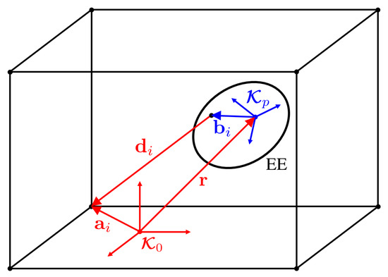
Figure 2.
Scheme of the closure equation of the i-th cable.
The inverse kinetostatic problem consists in solving Equation (2) to find the cable tensions. In rigid-body mechanics, this problem has, in general, solutions for a CDPR with redundant cables because there are n equilibrium equations and m unknowns. Since cables can only exert positive forces, all solutions involving negative tensions must be discarded. In many practical cases, it is desirable to maintain cable forces always higher than a lower limit greater than zero to prevent cables from becoming slack and smaller than a maximum value to avoid cable damage. One solution among the infinitely many possible can be chosen in order to achieve a suitable force distribution. In this paper, the inverse kinetostatic problem is solved by applying the method presented in [29], which is easily applicable in real time. In particular, the minimum 2-norm solution of the cable-tension array is used since this force distribution is continuous during a trajectory, and it minimizes cable forces.
2.2. Friction Model
To control cable forces without using any force sensor, the main problem is to find the correlation between the torque applied by the motor and the actual force applied on the end-effector, namely:
where is the drum radius, is the inertial torque produced by the moving parts of the winch (motor shaft, drum, …), is the torque generated by friction phenomena between the motor and the cable attachment point on the end-effector, and and are the cable velocity and acceleration, respectively. In the IPAnema 3 Mini robot, no gearboxes are used, so the drums are directly connected to the motor shafts. This means that the friction torque is generated only by the motor, the drum, and the pulleys. Figure 3 shows a scheme of one cable kinematic chain, representing the mechanical parts that generate the friction torque , including the location of the force sensor (a Futek LRM200 JR S-Beam load cell with a maximum load capacity equal to 25 lb). Since it is mounted on the third pulley, a friction force makes the measurement of the force different from the real one acting on the end-effector due to the friction between the third pulley and the cable attachment point to the end-effector. In general, and depend on both the cable force and velocity. The geometric and inertia properties of the mechanical parts of the winch are known, as well as the desired force (found by the force distribution algorithm). The motion law of the motor is computed through the robot inverse kinematics, which provides and . The motor motion law allows one to compute the inertial torque . Accordingly, the only unknown term in Equation (3) is . To determine this quantity, it is necessary to build a friction model by means of experimental tests.
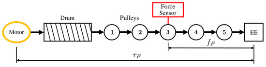
Figure 3.
Scheme of the robot kinematic chain and the areas in which the friction torque and force are modeled.
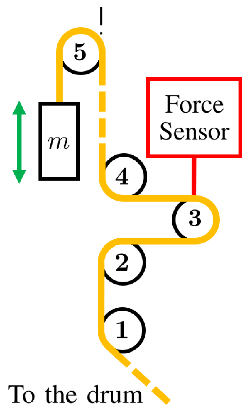
An experimental study was conducted on the kinematic chain of one winch (Figure 3) by detaching the cable from the end-effector. Different weights were attached to the cable: kg, kg, kg, kg, kg, kg, and kg. These values approximately cover the tension interval defined for the robot operation, from N to N. The weights were moved up and down with trajectories reaching several values of steady-state constant velocity: m/min, m/min, 1 m/min, 2 m/min, 3 m/min, 4 m/min, 5 m/min, and 6 m/min. The lower and higher velocities are called m/min and m/min. These values are the ones where only the portions of the motion laws with a constant velocity were analyzed. A scheme of the winch kinematic chain during the experiments is shown in Figure 4. Pulley 1 guides the cable arriving from the drum; pulleys 2, 3, and 4 are used to add the force sensor in the kinematic chain; pulley 5 guides the wire to the end-effector. During the constant-velocity portion of the motion, the term in Equation (3) is zero, and , where m is the mass of the weight attached to the cable, and g is the gravitational acceleration. The torque measured by the motor is saved, and its mean value is computed during different movements with the same constant velocity in the same direction. In this way, two different torques were obtained for each velocity and force of the cable, one for the movement in the positive direction and one for the movement in the negative direction. By inserting these torques in Equation (3) as , one can find the value of corresponding to a given velocity and cable tension for each motion direction. The distinction between the different movement directions is necessary since the results obtained with the experimental tests show different frictions in the two cases. The constant velocity used to build the friction model is the one set for the motor, whose value is supposed to be correct without the necessity of measuring the real velocity with an external sensor. This is acceptable since the velocity set for the motor will be used as an input of the final friction model in the control scheme.

Figure 4.
Scheme of the cable routing during the tests executed to estimate the parameters of the friction model in the cable actuation chain.
During the tests for the estimation of the friction model parameters, the cable routing in the first four pulleys is the same as in the working robot, so the friction that arises in this part of the kinematic chain is the same during the tests and during the robot operation. The same can be said for friction effects in the drum and the motor. However, this is not strictly true for friction effects in the last pulley of the kinematic chain. During testing, in fact, the wrapping angle is always equal to (see Figure 4). In contrast, during operation, this angle varies with the trajectory of the end-effector. Its value is always between and for the higher pulleys of the robot and between and for the lower ones. The approximation adopted for the estimation of friction parameters is, thus, better suited for the higher pulleys than for the lower ones. This is due to the fact that, in all the tested trajectories, the force-controlled cables (namely, the ones in which the friction model is applied) are the higher ones. The scheme shown in Figure 4 allows one to execute friction tests by only detaching the i-th cable from the end-effector without touching any other part of the robot. This means that friction tests can easily be executed whenever necessary (e.g., if some mechanical parts change or the friction parameters change in time due to wear of some components). This is the main advantage of the simplified friction model introduced in this section; its suitability will be assessed by the experiments reported in Section 4.
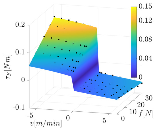
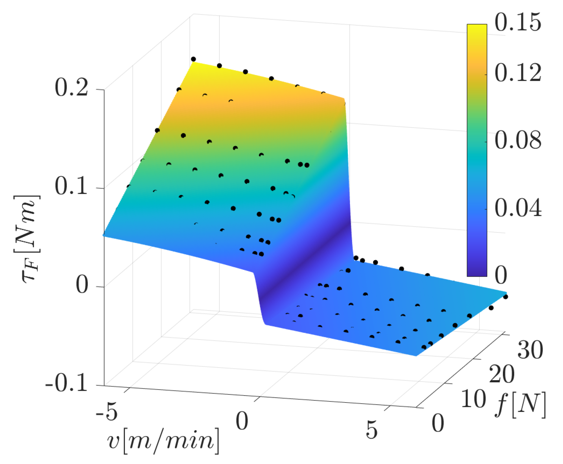
By analyzing the set of points obtained in the tests, we chose a model for estimating the friction torque that is linear in the force and parabolic in the velocity, namely,
The function shape at the right-hand side of Equation (4) is chosen as the best fit for the registered data. The shape is the same for the positive and negative motion directions, but the coefficients found through a best-fitting procedure differ. Since our experiments provide data to estimate dynamic friction only starting from the minimum velocity (the tests conducted with smaller velocities showed little repeatability, and thus, were considered unreliable), it is necessary to model the friction torque for velocities in the interval . This was achieved by using a polynomial with degree four in v for every force value, i.e., the polynomial coefficients are functions of f, and they are recomputed for every input force value. In this way, the complete model of the friction torque is
The 4 degrees of allow one to impose five conditions for the computation of coefficients :
- ; this condition is necessary to represent the behavior of the dynamic friction that is zero at rest (static friction is not modeled);
- continuity of the polynomial at the borders: and ;
- continuity of the derivative of the polynomial at the borders: , and .
The resulting coefficients are
The coefficients obtained for the friction torque model are listed in the first two rows of Table 1. These data are obtained by applying the Matlab function lsqnonlin with a step tolerance and a function tolerance both equal to . The lsqnonlin function implements a nonlinear least squares solver for curve-fitting problems, and it is used to find the coefficients and on the right-hand side of Equation (5) that minimize the 2-norm of the error vector between the friction torques computed with the model in Equation (5), and the torques recorded during the friction tests. Figure 5 represents the friction torque model described in Equation (5) with the coefficients listed in Table 1. The black points are the results provided by the experimental tests. The model is considered to give a good estimation of the physical phenomenon since the coefficient of determination [45] is higher than 0.9 (if , the function exactly interpolates the input data). It is interesting to note that the maximum value of the predicted friction torque is Nm, which is approximately of the nominal motor torque (equal to Nm). This suggests the importance of the friction model introduced in this section.

Experimental tests were carried out to develop a customized friction model for each winch of the robot, but the results obtained on the control of the overall robot do not show an appreciable improvement in performance compared to the use of the same friction model for all winches (as long as all the winches and the kinematic chains between the drums and the attachment points on the end-effector are the same). For this reason, the same friction model developed on one winch was applied to all the winches. The details of this analysis are not reported for the sake of brevity.
During the tests executed for developing the friction torque model, the data recorded by the load cell mounted in the kinematic chain (Figure 3) were saved. These data allowed us to derive a model for the friction force . This model is analogous to that in Equation (5), with replacing and distinct coefficients (third and fourth rows of Table 1):
Using a friction model to correct the force measured by the load cells is necessary to obtain an accurate estimation of the actual force acting on the cable attachment point [43]. The measured forces are not used for the new control algorithms described in this paper, but they were exploited during the validation experiments described in Section 4.
2.3. Following-Error Model
As an alternative to using the motor torque in the feedback loop to control the cable forces (see Section 3), we propose using the so-called following-error (FE), which is the difference between the position set for the motor and the actual one. This is because the torque that the motor measures is usually noisy, and it must be filtered before it can be used in a feedback control loop. Filtering the torque means introducing a delay, which could be a problem for fast movements. The FE has a noisy behavior too, but its oscillations are usually appreciably smaller than the torque ones. Our experiments show that the FE can be used in a feedback loop without any filter.
The IPAnema 3 Mini is equipped with Beckhoff servomotors AM3121-0201 connected to Beckhoff EL7201 terminals, which receive inputs from a programmable logic control (PLC) program developed in TwinCAT 3.1 and running with a cycle time of 1 ms. The motors are controlled in velocity (i.e., a velocity command is given to the motor by the PLC program every millisecond), with a PI controller at the drive level. The position feedback loop is closed in the PLC program with a different P controller that was untouched in this work. If the integral part of the PI controller of the drive is removed, a pure proportional controller designed only through its gain acts on the motor. In this configuration, when an external torque is applied to the motor shaft, the latter moves to a position that allows the motor torque to balance the external one. Due to the proportional nature of the control law, the position reached by the motor is different from the commanded one, so that an FE arises. In practice, the motor behaves as a torsional spring: an FE on the shaft gives a specific torque and vice versa. This behavior was modeled through experimental tests similar to those used to model the friction torque. In this case, the tests were executed in a static way by applying different loads to the cable with different values of . By recording the motor torque and the motor FE for every test, a set of FE points (every one corresponding to a given torque and a given ) is found, which provides, through a best-fit procedure, the coefficient in the static model reported below (Figure 6):
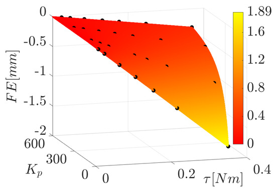
Figure 6.
FE model described in Equation (8).
However, Equation (8) is insufficient to model the FE during a movement. Indeed, while executing the dynamic tests to model the friction torque, the FE was also recorded. Even though in those tests, the complete PI controller at the drive level was used, an FE approximately proportional to the cable velocity (and not influenced by the applied force) was observed. The corresponding coefficient was obtained through a best-fit procedure.
To obtain the final model of the FE, the terms depending on the torque and the cable velocity are summed together:
In this work, is always equal to 200. This default value was considered appropriate to avoid a transmission that is too stiff (with a higher ) or too compliant (with a smaller ). Tests with different values of were performed, but they are not reported here for the sake of brevity.
In the experimental tests, the FE is computed as a difference between the actual cable length and the commanded one. So it is measured in meters, as a length. The values of the coefficients and are found with the same procedure used for the computation of the friction model coefficients, i.e., by using the Matlab function lsqnonlin with a step tolerance and a function tolerance both equal to . Their values are , and , with expressed in newtons per meter and v in meters per minute. These values lead to a coefficient of determination of the FE model equal to 0.999. The coefficients and differ by several orders of magnitude, but the value that multiplies in Equation (9) is . Working with coefficients with this order of magnitude was not a problem since double-precision variables were used in the PLC code.
3. Hybrid Control Strategy
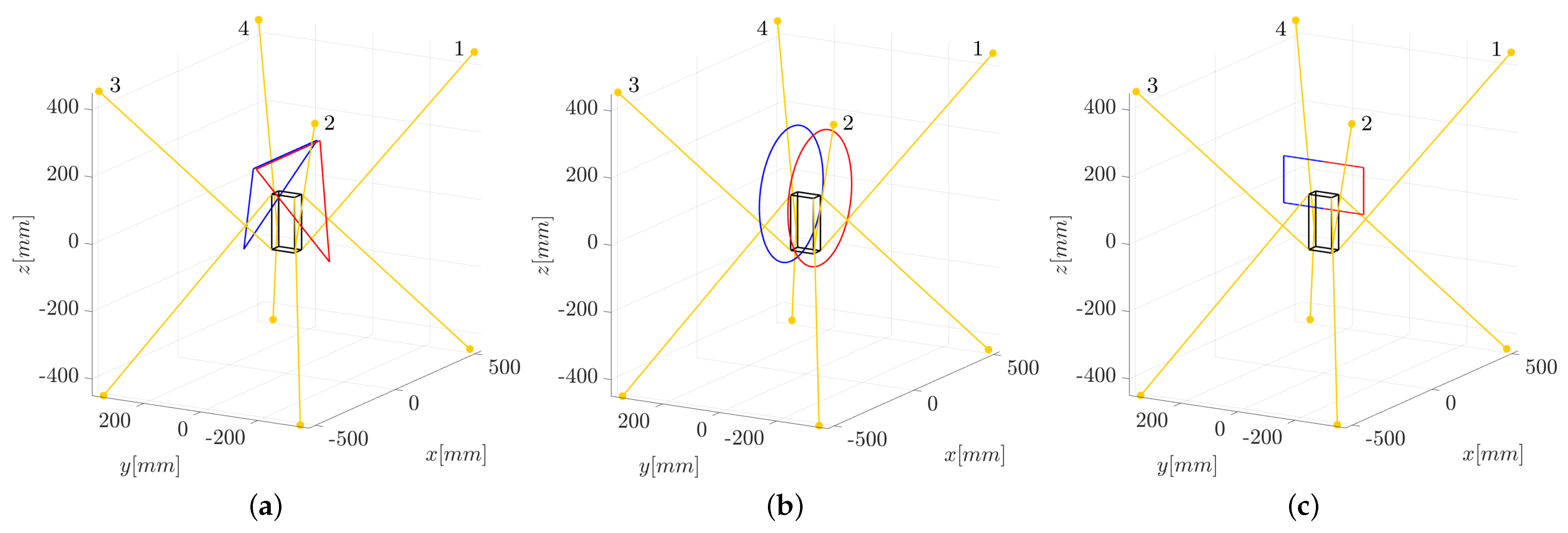
For the HC strategy adopted in this paper, the first step is to choose the pair of cables to be force-controlled for a given pose of the end-effector or a given trajectory. To achieve this, the force distribution sensitivity index introduced in [40] is computed for every possible pair of cables i and j of the IPAnema 3 Mini. We choose to force control the pairs of cables and because they guarantee N in large parts of the robot constant-orientation workspace, as shown in Figure 7 (in this paper, the end-effector orientation is always described by the rotation matrix , where is the identity matrix). Choosing a pair of force-controlled cables with a small (values of smaller than 2 N can be considered practically acceptable [41]) helps to minimize the errors in the achieved force distribution.
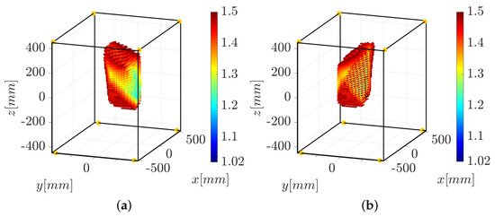
Figure 7.
Workspace of the IPAnema 3 Mini with N when the force-controlled cables are (a) or (b). The yellow dots represent the exit points of the cables from the frame.
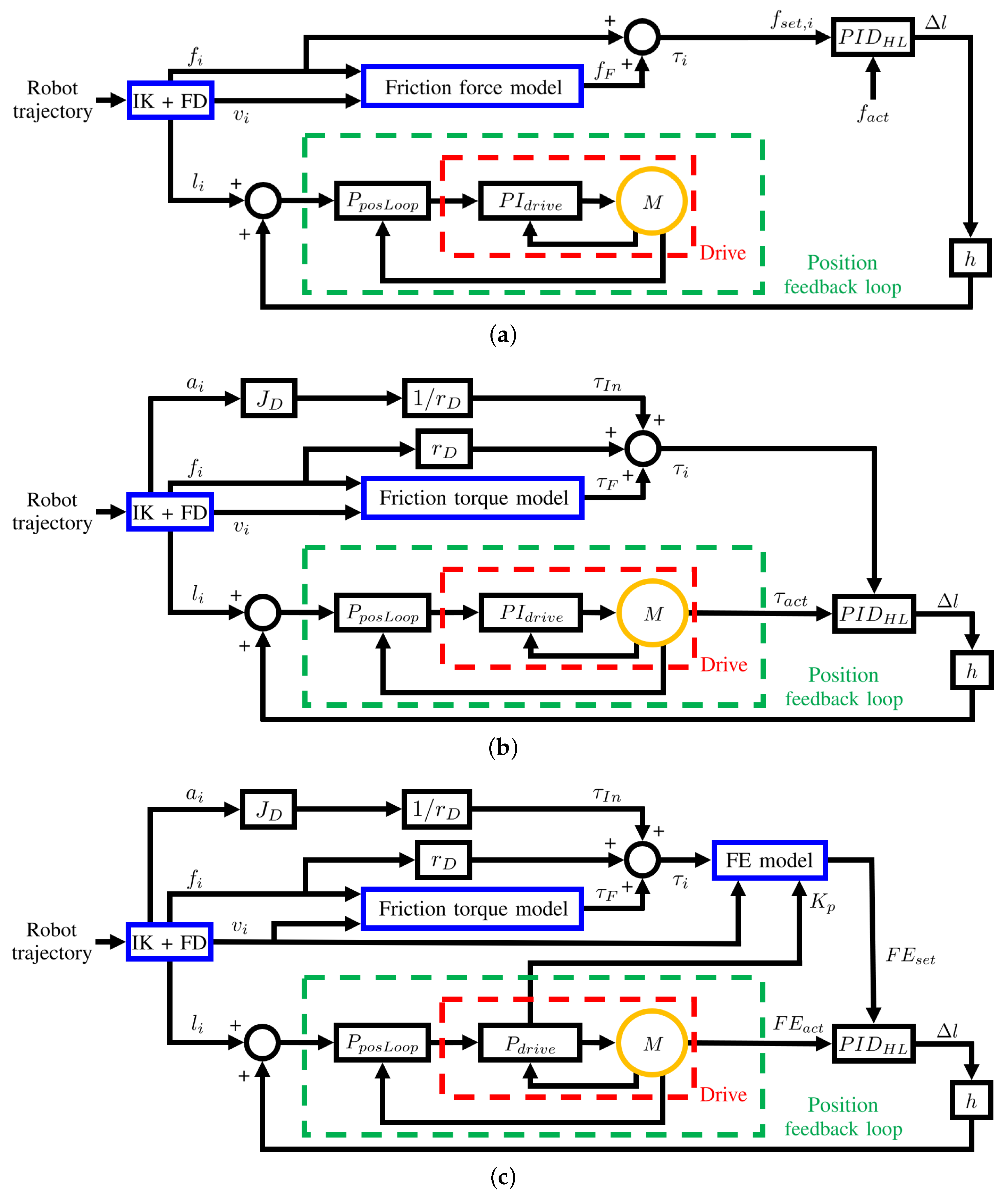
Once the force-controlled cables are identified, it is necessary to define the control strategy that acts on these wires to obtain the desired forces. Figure 8 shows three schemes in which the subscript “i” refers to the generic i-th cable. All of them present a high-level PID controller () which computes the value to be added to the cable length after a multiplication with a scaling factor h. The locution “high-level” is used to differentiate this controller from the ones that act on the motor at the drive level. The controllers differ in the variables that are given to as input for the computation of : a force in HC-f (Figure 8a), a torque in HC- (Figure 8b), and an FE in HC-e (Figure 8c). For all controllers, is computed (as the cable velocity and acceleration ) by the robot inverse kinematics (IK). The force desired in the i-th cable is computed by the force distribution algorithm. The scaling factor h is always in the interval , and it is modified only during the activation or deactivation phases of the controller or when changing the pair of cables to force-controlled, according to the function
starts from 0 when the controller is activated and it is increased at every iteration by until it reaches (or exceeds) . Then, is held constantly equal to () until the force control is deactivated. When the controller is switched off, is subtracted until reaches (or exceeds) 0. To change the force-controlled cables, it is sufficient to switch on the force control in the new cables and switch it off in the old ones. The shape of the function on the right-hand side of Equation (10) is chosen in order to have a smooth transition of the coefficient h from 0 to 1 during the activation and deactivation of the controller.
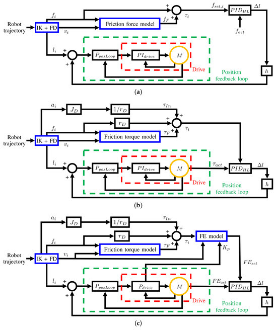
Figure 8.
Control schemes applied to force-controlled cables by using (a) force sensor feedback, HC-f; (b) motor-torque feedback, HC-; and (c) FE feedback, HC-e.
The scheme in Figure 8a (HC-f) is the simplest, and it represents the situation in which force sensors are used. In this case, is the force measured by the load cell mounted in the kinematic chain of cable i. The high-level PID controller compares with the desired one , which is computed by correcting the output force of the force distribution algorithm with the friction force estimated through the model in Equation (7). For the computation of , the theoretical values and are used because they yield non-noisy results. Once the cable length is corrected with , it is fed to the proportional controller for the position feedback loop () in the PLC, which computes a reference velocity to give as input to the PI controller () of the motor (M) drive. The position-controlled cables do not need the computation of , so in this case, is directly input into .
The scheme in Figure 8b (HC-) is the first to force-control cable i without using the load cell. Here, the high-level PID controller takes as input the actual torque given by the motor and the torque that we wish to command to the motor to obtain force in the cable. is computed using Equation (3), where the friction torque is estimated by the model in Equation (5). is the inertia of all the moving parts connected to the motor shaft.
Finally, the scheme in Figure 8c (HC-e) allows control of the cable i by force by using the motor FE. Here, after the computation of torque , the model in Equation (9) is used to compute the FE that is desired on motor i () to generate force . This FE is one of the two inputs of the high-level PID controller, while the other is the actual FE measured by the motor (). In this case, a pure proportional controller with a gain is used at the drive level (). It is interesting to note that, in this case, the position-controlled cables that can be switched to force-controlled during the robot motion must also have a pure proportional controller at the drive level to not change the controller of the drive online. This can cause a small error in the length of the position-controlled cables, but in practice this phenomenon did not affect robot accuracy (see Section 4).
The first tests of the HC were executed on a simple test bench with only two cables. One of the two cables is position-controlled, whereas the other is force-controlled by imposing a specific tension. In this configuration, all control schemes shown in Figure 8 were tested to tune the controller parameters with a heuristic procedure based on the Ziegler–Nichols method [46]. The transfer function that describes the high-level PID controller in the Laplace domain is
The parameters to be identified are the proportional gain , the integral action time , the derivative action time , and the damping time . The values found for the three controllers shown in the schemes of Figure 8 are listed in Table 2. When , and thus , the derivative part of the controller is switched off and it becomes a PI controller. This happens for the controllers HC- and HC-e, because the values of FE and torque given by the motor (even if the torque is smoothed with a filter) are affected by some noise and using noisy inputs in the controller when the derivative part is switched on results in unwanted vibrations on the motor shaft.
Table 2.
Parameters of the three different high-level PID controllers shown in Figure 8.
4. Experimental Results and Validation
Since the friction model introduced in Section 2.2 is valid only for dynamic friction, the main problem of the controllers HC- and HC-e is the lack of precision in predicting the forces when the robot platform is at rest. The situation is different when the load cells are used because, even if the static friction is not modeled for the correction of cable forces, the static force measures are still rather precise. However, for applications in which the robot is moving most of the time or where it is not required to exert specific static wrenches with the end-effector, it is only important to maintain the cables taut to prevent them from becoming slack during motion.
Accordingly, the tests are executed on dynamic trajectories (shown in Figure 9) assigned to the end-effector. One triangular and one circular motion law are defined in the workspace of the robot with N (Figure 7a), and the other two in the workspace of the robot where N (Figure 7b). The rectangular motion law is built so it passes through the plane , so that the pair of force-controlled cables must be changed during the execution of the movement. The paths where the force-controlled cables are wires 1 and 2 are plotted in red, whereas the paths in which the force-controlled cables are 3 and 4 are plotted in blue. All trajectories are purely translational motions, and they represent the movement of the center of the reference system . Though different platform velocities were tested, in all motion laws shown in this paper, for the sake of comparison, the end-effector reaches a velocity of 4 m/min after the first acceleration from a static position.
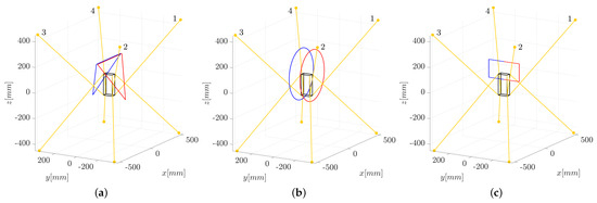
Figure 9.
Robot trajectories in the experimental tests. The paths where the force-controlled cables are wires are plotted in red, whereas the ones in which the force-controlled cables are wires are plotted in blue. (a) Triangular trajectories (b) Circular trajectories (c) Rectangular trajectory.
The force limits defined for the robot are N and N. In order to keep some margin with respect to force oscillations and imprecision in the robot geometry or wrench estimation, a minimum tension equal to 8 N is considered for the computation of the force distribution. The wrench exerted on the end-effector is simply the one due to its weight and inertia, which is computed from the platform mass ( kg).
The forces plotted in Figure 10, Figure 11, Figure 12 and Figure 13 are the ones measured by the built-in load cells corrected with the dynamic friction model described by the coefficients in the third and fourth lines of Table 1.
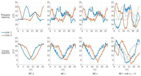
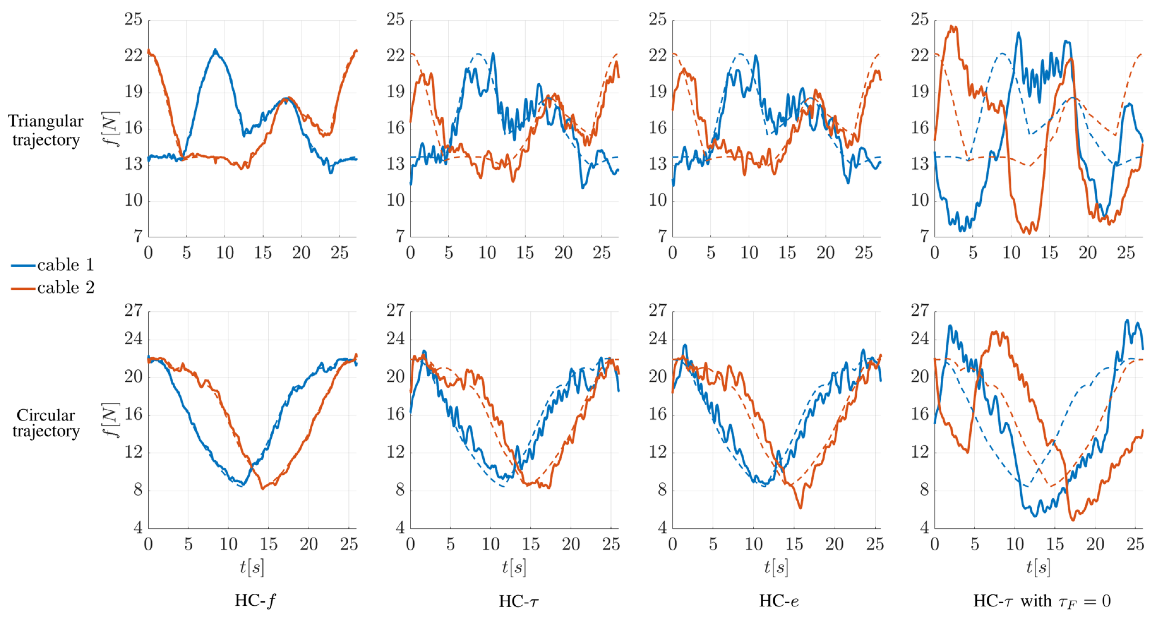
Figure 10.
Examples of the evolution in time of the cable tensions in the force-controlled cables for the triangular (plots in the first row) and circular (plots in the second row) red trajectories in Figure 9. Different controllers are considered: controller HC-f, controller HC-, controller HC-e, controller HC- without the friction torque model. Solid lines represent measured forces, whereas dashed lines represent the theoretical forces computed through the force distribution algorithm.
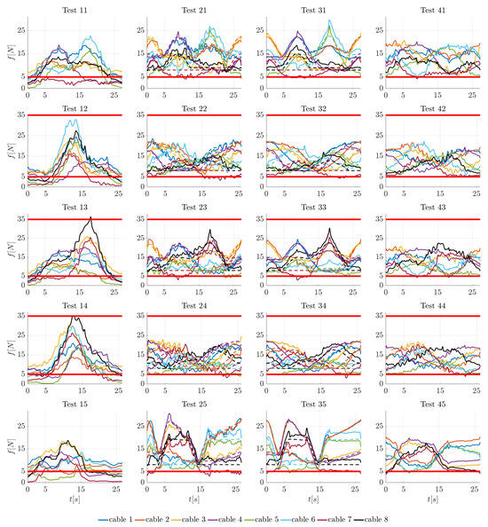
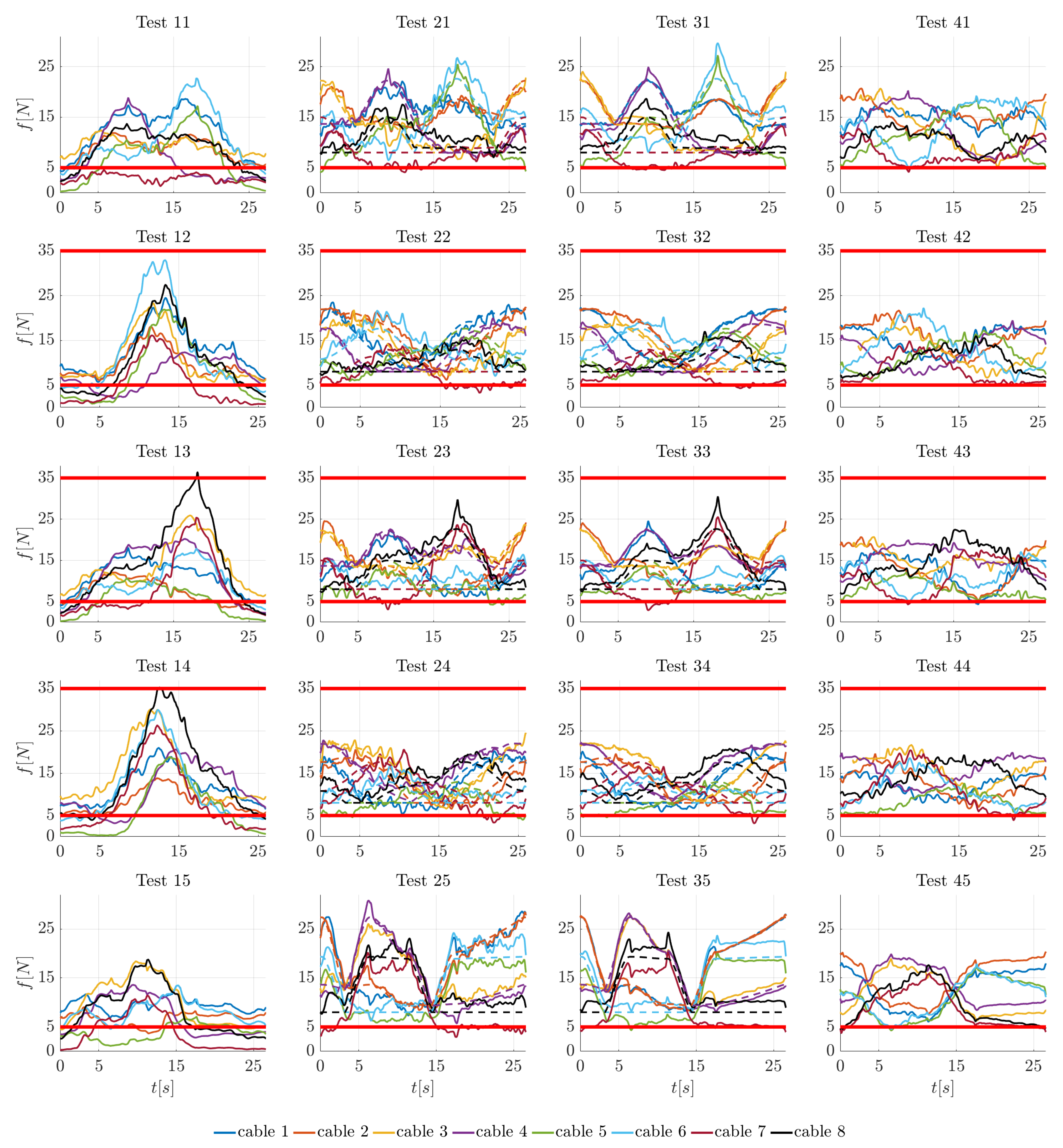
Figure 11.
Evolution in time of the cable forces during the tests identified by the legend in Table 3. N and N are the desired bounds of cable tensions. Solid lines represent measured forces, whereas dashed lines represent the theoretical forces computed through the force distribution algorithm.
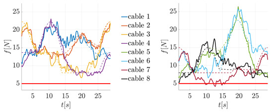
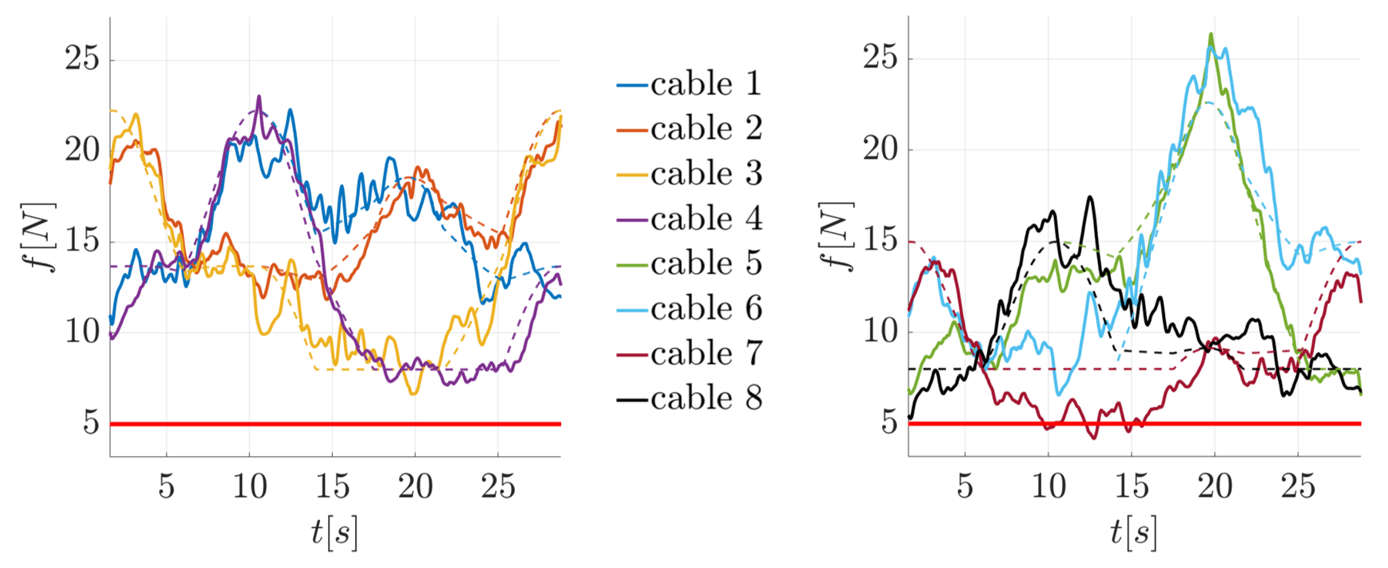
Figure 12.
Evolution in time of the cable forces in test 51.
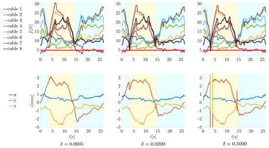
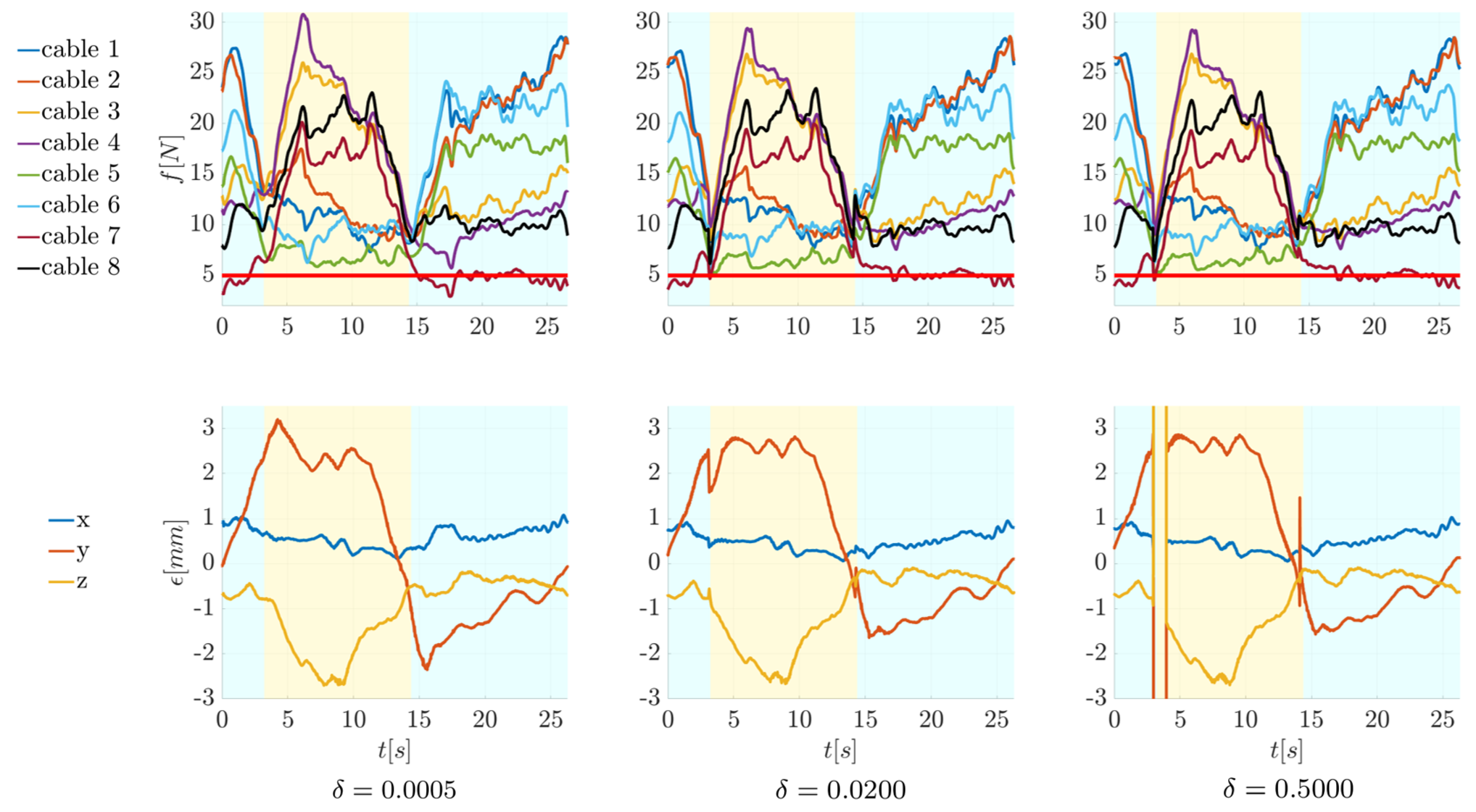
Figure 13.
The plots show the evolution in time of cable forces (plots in the first row) and position error (plots in the second row) when force-controlled cables are changed for increasing values of . The areas in light blue represent the parts of the trajectory in which the force-controlled cables are 1 and 2, while the areas in yellow are the ones in which the force-controlled cables are 3 and 4.
4.1. Comparison between the Hybrid Control Strategies
Figure 10 shows the evolution in time of the forces in the force-controlled cables for the triangular (plots in the first row) and circular (plots in the second row) red trajectories in Figure 9. When the controller HC-f (Figure 8a) is used, the measured forces (solid lines) track the theoretical ones (dashed lines) computed through the force distribution algorithm very well. The results obtained with the controllers HC- (Figure 8b) and HC-e (Figure 8c) are similar: in both cases the actual forces are noisy compared to the theoretical ones, but the evolution in time of the tensions is approximately followed. These behaviors of the forces when applying the three controllers are observed also for different trajectories (e.g., for the blue ones in Figure 9). In particular, the similarity between the forces generated by the HC- controller and the HC-e controller suggests that there is no practical difference in applying one controller rather than the other for the motion laws studied in this work. However, these results are obtained by using a filtered motor torque, and the raw value of the motor FE in the feedback loop. As mentioned in Section 2.3, filtering the torque could be a problem for faster movements and, in this case, the HC-e controller could provide an advantage.
The plots in the last column of Figure 10 show the effect of setting in Equation (3), namely, neglecting the friction model in the HC- controller. It is clear that force tracking becomes considerably worse. Moreover, in this case, one or more tensions in the position-controlled cables go below the desired minimum value (5 N), which is not acceptable. Analogous results are obtained if friction is neglected in the HC-e controller, which confirms the necessity to model friction in the kinematic chains.
4.2. Comparison between the Hybrid Controllers and Other Controllers
To evaluate the performance of the controller proposed in this paper, the results obtained by applying it to different trajectories are compared to the ones gained with different controllers. The legend shown in Table 3 is used to identify the executed trajectory and the controller applied in every test. The first number represents the controller used during the execution of the motion law. The controller HC-e is compared with HC-f, with the nullspace control (NC) presented in [4] (which was already developed and tested on the IPAnema 3 Mini) and with a pure inverse kinematic controller (IKC). The latter is the only method besides HC-e that does not exploit force sensors (the IKC is a pure position controller based on robot inverse kinematics, without any action on the cable tensions). The second number in Table 3 identifies the trajectory among those shown in Figure 9.
In evaluating the controllers’ performances, the evolution in time of the cable forces, the precision, and the repeatability of the robot are taken into account. For the estimation of the robot accuracy and repeatability, the position of a marker mounted on the end-effector is measured with a Leica AT960 laser tracker, which guarantees an absolute accuracy of . The experimental setup configuration is the same as used in [4], so we can estimate an accuracy of , while the sampling rate of the measurements is 1000 Hz.
Figure 11 represents the evolution in time of the cable forces. During the tests 1j () executed with the controller IKC, there is no control over the cable tensions, so for large parts of the movements there is at least one cable force that is smaller than the minimum tension (5 N). Moreover, in tests 13 and 14, the force on cable 8 exceeds the maximum limit of 35 N. Without any control over cable tensions it is impossible to guarantee that they remain within the given limits. On the contrary, with the same hardware (that does not exploit the load cells for control aims), the controller HC-e allows the cable forces to be maintained within the predefined limits for most of the movement. During tests 2j (), only for a few instants one cable tension slightly drops under the lower limit. When applying the HC-f controller, which makes use of load cells, the situation is very similar. As a matter of fact, in tests 3j (), the most relevant difference compared to tests is that the better tracking of tensions in the force-controlled cables produces less noisy forces in all cables. For the same motion law, the points at which the tensions drop under 5 N when the HC-f is applied are approximately the same as when the HC-e is applied. As expected, the main errors between the theoretical forces computed through the force distribution algorithm and the real ones are in the position-controlled cables. When the NC controller is applied, in tests 4j (), the forces do not follow the theoretical values computed through a force distribution algorithm. The controller maintains them as close as possible to the mean value N and corrects them when they become lower than N. The results are forces slightly smaller during the movement, but their oscillations are more similar to the ones obtained with the HC-e than those with the HC-f. In this case, the lower limit N is almost always respected during the motion.
Table 4 shows the results in terms of accuracy obtained during the same tests as shown in Figure 11. The values in the table represent the absolute error (expressed as a Cartesian distance) in the position of the marker between the set trajectory and the executed one. The maximum and mean error over an entire motion law measure the accuracy. The results are always similar for tests 1j, 2j, 3j, and 4j, with an error in the positioning of the marker that has a maximum value between mm and mm and a mean value between mm and mm. The differences in using different controllers are on the order of tenths of a millimeter. They vary for different motion laws, so that we can consider all controllers equivalent in terms of accuracy. Note that when the robot is controlled by the IKC controller, one or more cables can become slack and this significantly degrades the achieved accuracy with respect to that reported in Table 4. This was experienced in a number of other tests (depending on the initial pre-tensioning of cables), that are not reported for the sake of brevity.
Table 4.
Robot accuracy with several controllers applied to different trajectories. The errors in the positioning of the marker are evaluated for a given test through the maximum () and mean () value over an entire motion law.
Test 51 is the last in Table 4 that needs to be analyzed. Here, the triangular red trajectory of Figure 9a is executed, but the controller is different from the others previously described. The control scheme shown in Figure 8c is applied to all cables (i.e., all cables are force-controlled without using load cells). Better force tracking than with HC-e is achieved in all cables, as we can see in Figure 12. However, applying force control in all cables results in poor manipulator accuracy, with a maximum position error of mm, as shown in Table 4.
Finally, the repeatability of the robot is evaluated by executing the triangular trajectory for force-controlled cables with the different controllers (tests 11, 21, 31, 41). The repeatability is measured by computing the standard deviation of the errors in Table 4 over 15 consecutive executions of the same motion law. Table 5 lists the maximum and mean values. The controller does not seem to have a high influence on the repeatability of the manipulator, even if a slightly better repeatability is obtained with the NC controller.
Table 5.
Repeatability in mm over 15 consecutive trajectories.
4.3. Effect of Changing the Pair of Force-Controlled Cables
Some tests were conducted to analyze the effect of changing the pair of force-controlled cables during the execution of a trajectory. For this purpose, the rectangular motion law in Figure 9c is considered. The change in the force-controlled cables is managed as described in Section 3 through the value of the scaling factor h in Equation (10). While cables 5, 6, 7, and 8 are always position-controlled, the scheme shown in Figure 8c is applied to all the first four cables. When the pair of force-controlled cables is switched, the value of h goes from zero to one in the cables on which the force control is activated and vice versa in the cables on which the force control is deactivated. In Figure 13, the effect of increasing is analyzed on the evolution in time of the forces and the position error. The areas in light blue represent the parts of the trajectory in which the force-controlled cables are 1 and 2, while the areas in yellow are the ones in which the force-controlled cables are 3 and 4. The controller used for these tests is always HC-e.
When , the change is very smooth and slow, with a smooth behavior in the forces and the position error as well. The more rapid the change in the value of h ( higher), the more the applied to the length of the i-th cable is similar to a step. The time necessary for the change in the force-controlled cables can be computed from Equation (10) by considering that must reach (or exceed) starting from zero with an increment equal to every millisecond (the cycle time of the PLC program). When , the change happens in 3142 ms; when , it takes 79 ms; finally, when , the change is almost a step since it takes only 4 ms. For or , even though the forces quickly drop during the change, they do not become smaller than 5 N; however, the command given to the motor produces a sudden change in the position of the platform that is visible in the plots of the errors (difference between the set position and the executed one). Values of between 0.0005 and 0.02 seem appropriate for the executed tests.
5. Conclusions
This work extends the hybrid position–force control strategy (HC) that was first introduced in [38,39] and later enhanced in [40,41] for overconstrained CDPRs with n DOFs: n cables of the robot are position-controlled, whereas the redundant cables are force-controlled. The main contribution of this work was to apply the HC without using force sensors, which decreases the hardware complexity and cost. To this aim a simple friction model was used to estimate the correlation between the force applied to a cable and the torque given by the motor. Also, a model was introduced for estimating the motor following-error (FE) for a given motor torque when a pure proportional controller is used at the drive level.
Two controllers were proposed: the first one uses the motor torque as an input (HC-), while the second exploits the motor FE (HC-e). Using the FE or the torque in the feedback loop gave similar results in the tests executed in this work for rather slow trajectories. It is conjectured that HC-e may work better for fast movements, but confirming this will be the objective of future research. The results obtained in the experimental tests on several motion laws show good behavior of the HC-e controller when compared to the classical HC-f approach applied in [38,39,40] or the nullspace control method (NC) presented in [4], both of which exploit the readings of force sensors mounted in the robot. Cable force tracking was accurate enough to keep the tensions within the force limits. The HC-e controller proved much more effective than a pure inverse kinematic controller (IKC), the only other method that does not use load cells for control purposes. IKC could not guarantee to maintain cable forces within the given limits. The accuracy and repeatability obtained with the HC-e controller were almost the same as the other two methods that use force sensors: the mean value of the maximum error over the considered trajectories was mm for the HC-e controller, mm for the HC-f controller, and mm for the NC controller. Finally, the effect of changing the pair of force-controlled cables during the robot movement was analyzed, demonstrating that this change can be effectively performed as long as a smooth transition is commanded.
Future developments are necessary to prove the effectiveness of the proposed control strategy for robots executing faster movements, which will be the objective of our future research. The simple friction model described in Section 2.2 gave good results for the tests shown in Section 4. This model is particularly suitable for practical applications because it is possible to easily repeat the friction tests whenever necessary. However, it is not certain that the same model would be suitable for highly dynamical motions. In this case, a more precise and complex friction model (e.g., taking into account friction in the pulley bearings or the influence of different wrapping angles of cables on pulleys) could be necessary for better controller performance. These contributions, as well as the introduction of a model for static friction, will be evaluated in future studies.
Finally, the tuning of the PID parameters in the HC-e and HC- controllers could be analyzed to improve their performance, since the values reported in Table 2 were found through a trial-and-error procedure based on the Ziegler–Nichols approach [46]. For the aim of this work, these values seem appropriate, but motions involving higher velocities and accelerations could require a different and better PID controller tuning. This analysis, as well as deeper studies related to the stability of the proposed controllers, are deferred to future studies.
Author Contributions
Conceptualization, A.B. and E.M.; methodology, A.B. and L.G.; software, L.G., M.F. and C.M.; validation, L.G.; formal analysis, L.G.; investigation, L.G.; resources, M.F. and C.M.; data curation, L.G.; writing—original draft preparation, L.G.; writing—review and editing, L.G. and M.C.; visualization, L.G. and M.C.; supervision, A.B. and M.C.; project administration, M.C.; funding acquisition, A.B. and M.C. All authors have read and agreed to the published version of the manuscript.
Funding
This research received no external funding.
Data Availability Statement
Data are contained within the article.
Acknowledgments
This work was supported by Marchesini Group S.p.A., a leading company in the field of automatic packaging machines, especially for pharmaceutical and cosmetic products.
Conflicts of Interest
Authors Alessandro Berti and Eros Monti were employed by the company Marchesini Group S.p.a. The remaining authors declare that the research was conducted in the absence of any commercial or financial relationships that could be construed as a potential conflict of interest.
Abbreviations
The following abbreviations are used in this manuscript:
| CDPR | Cable-driven parallel robot |
| DOFs | Degrees of freedom |
| HC | Hybrid joint-space control |
| NC | Nullspace control |
| IKC | Inverse kinematic controller |
| FE | Following-error |
References
- Pott, A. Cable-Driven Parallel Robots: Theory and Application, 1st ed.; Springer: Cham, Switzerland, 2018. [Google Scholar] [CrossRef]
- Idà, E.; Mattioni, V. Cable-Driven Parallel Robot Actuators: State of the Art and Novel Servo-Winch Concept. Actuators 2022, 11, 290. [Google Scholar] [CrossRef]
- Pott, A.; Mütherich, H.; Kraus, W.; Schmidt, V.; Miermeister, P.; Verl, A. IPAnema: A family of Cable-Driven Parallel Robots for Industrial Applications. In Cable-Driven Parallel Robots; Bruckmann, T., Pott, A., Eds.; Springer: Berlin/Heidelberg, Germany, 2013; pp. 119–134. [Google Scholar] [CrossRef]
- Fabritius, M.; Rubio-Gómez, G.; Martin, C.; Santos, J.C.; Kraus, W.; Pott, A. A nullspace-based force correction method to improve the dynamic performance of cable-driven parallel robots. Mech. Mach. Theory 2023, 181, 105177. [Google Scholar] [CrossRef]
- Bruckmann, T.; Lalo, W.; Nguyen, K.; Salah, B. Development of a Storage Retrieval Machine for High Racks Using a Wire Robot. In Proceedings of the ASME 2012 International Design Engineering Technical Conferences and Computers and Information in Engineering Conference, Chicago, IL, USA, 12–15 August 2012; pp. 771–780. [Google Scholar] [CrossRef]
- Bruckmann, T.; Sturm, C.; Fehlberg, L.; Reichert, C. An energy-efficient wire-based storage and retrieval system. In Proceedings of the 2013 IEEE/ASME International Conference on Advanced Intelligent Mechatronics, Wollongong, NSW, Australia, 9–12 July 2013; pp. 631–636. [Google Scholar] [CrossRef]
- Reichert, C.; Bruckmann, T. Optimization of the Geometry of a Cable-Driven Storage and Retrieval System. In Proceedings of the International Symposium on Robotics & Mechatronics 2017, Sydney, Australia, 29 November–1 December 2017; pp. 225–237. [Google Scholar] [CrossRef]
- Zhang, F.; Shang, W.; Zhang, B.; Cong, S. Design Optimization of Redundantly Actuated Cable-Driven Parallel Robots for Automated Warehouse System. IEEE Access 2020, 8, 56867–56879. [Google Scholar] [CrossRef]
- Izard, J.B.; Gouttefarde, M.; Baradat, C.; Culla, D.; Sallé, D. Integration of a Parallel Cable-Driven Robot on an Existing Building Façade. In Cable-Driven Parallel Robots; Bruckmann, T., Pott, A., Eds.; Springer: Berlin/Heidelberg, Germany, 2013; pp. 149–164. [Google Scholar] [CrossRef]
- Hussein, H.; Santos, J.C.; Gouttefarde, M. Geometric Optimization of a Large Scale CDPR Operating on a Building Facade. In Proceedings of the 2018 IEEE/RSJ International Conference on Intelligent Robots and Systems (IROS), Madrid, Spain, 1–5 October 2018; pp. 5117–5124. [Google Scholar] [CrossRef]
- Pusey, J.; Fattah, A.; Agrawal, S.; Messina, E. Design and workspace analysis of a 6-6 cable-suspended parallel robot. Mech. Mach. Theory 2004, 39, 761–778. [Google Scholar] [CrossRef]
- Gouttefarde, M.; Collard, J.F.; Riehl, N.; Baradat, C. Geometry Selection of a Redundantly Actuated Cable-Suspended Parallel Robot. IEEE Trans. Robot. 2015, 31, 501–510. [Google Scholar] [CrossRef]
- Surdilovic, D.; Bernhardt, R. STRING-MAN: A new wire robot for gait rehabilitation. In Proceedings of the IEEE International Conference on Robotics and Automation, ICRA ’04, New Orleans, LA, USA, 26 April–1 May 2004; Volume 2, pp. 2031–2036. [Google Scholar] [CrossRef]
- Lamine, H.; Laribi, M.A.; Bennour, S.; Romdhane, L.; Zeghloul, S. Design Study of a Cable-based Gait Training Machine. J. Bionic Eng. 2017, 14, 232–244. [Google Scholar] [CrossRef]
- Ben Hamida, I.; Laribi, M.A.; Mlika, A.; Romdhane, L.; Zeghloul, S.; Carbone, G. Multi-Objective optimal design of a cable driven parallel robot for rehabilitation tasks. Mech. Mach. Theory 2021, 156, 104141. [Google Scholar] [CrossRef]
- Picard, E.; Caro, S.; Plestan, F.; Claveau, F. Stiffness Oriented Tension Distribution Algorithm for Cable-Driven Parallel Robots. In Advances in Robot Kinematics 2020; Lenarčič, J., Siciliano, B., Eds.; Springer International Publishing: Cham, Switzerland, 2021; pp. 209–217. [Google Scholar] [CrossRef]
- Kawamura, S.; Choe, W.; Tanaka, S.; Pandian, S. Development of an ultrahigh speed robot FALCON using wire drive system. In Proceedings of the 1995 IEEE International Conference on Robotics and Automation, Nagoya, Japan, 21–27 May 1995; Volume 1, pp. 215–220. [Google Scholar] [CrossRef]
- Kawamura, S.; Kino, H.; Won, C. High-speed manipulation by using parallel wire-driven robots. Robotica 2000, 18, 13–21. [Google Scholar] [CrossRef]
- Dekker, R.; Khajepour, A.; Behzadipour, S. Design and testing of an ultra-high-speed cable robot. Int. J. Robot. Autom. 2006, 21, 25–34. [Google Scholar] [CrossRef]
- Zhang, Z.; Shao, Z.; Wang, L.; Shih, A.J. Optimal Design of a High-Speed Pick-and-Place Cable-Driven Parallel Robot. In Cable-Driven Parallel Robots; Gosselin, C., Cardou, P., Bruckmann, T., Pott, A., Eds.; Springer: Cham, Switzerland, 2018; pp. 340–352. [Google Scholar] [CrossRef]
- Zhang, Z.; Shao, Z.; Wang, L. Optimization and implementation of a high-speed 3-DOFs translational cable-driven parallel robot. Mech. Mach. Theory 2020, 145, 103693. [Google Scholar] [CrossRef]
- Guagliumi, L.; Berti, A.; Monti, E.; Carricato, M. Design Optimization of a 6-DOF Cable-Driven Parallel Robot for Complex Pick-and-Place Tasks. In Proceedings of the ROMANSY 24—Robot Design, Dynamics and Control, Udine, Italy, 4–7 July 2022; Kecskeméthy, A., Parenti-Castelli, V., Eds.; Springer: Cham, Switzerland, 2022; pp. 283–291. [Google Scholar] [CrossRef]
- Ouyang, B.; Shang, W. Rapid optimization of tension distribution for cable-driven parallel manipulators with redundant cables. Chin. J. Mech. Eng. 2016, 29, 231–238. [Google Scholar] [CrossRef]
- Jamshidifar, H.; Khajepour, A.; Fidan, B.; Rushton, M. Kinematically-Constrained Redundant Cable-Driven Parallel Robots: Modeling, Redundancy Analysis, and Stiffness Optimization. IEEE/ASME Trans. Mechatron. 2017, 22, 921–930. [Google Scholar] [CrossRef]
- Côté, A.F.; Cardou, P.; Gosselin, C. A tension distribution algorithm for cable-driven parallel robots operating beyond their wrench-feasible workspace. In Proceedings of the 2016 16th International Conference on Control, Automation and Systems (ICCAS), Gyeongju, Republic of Korea, 16–19 October 2016; pp. 68–73. [Google Scholar] [CrossRef]
- Pott, A.; Bruckmann, T.; Mikelsons, L. Closed-form Force Distribution for Parallel Wire Robots. In Proceedings of the 5th International Workshop on Computational Kinematics, Duisburg, Germany, 6–8 May 2009; Kecskeméthy, A., Müller, A., Eds.; Springer: Berlin/Heidelberg, Germany, 2009; pp. 25–34. [Google Scholar] [CrossRef]
- Pott, A. An Improved Force Distribution Algorithm for Over-Constrained Cable-Driven Parallel Robots. In Proceedings of the 6th International Workshop on Computational Kinematics, Barcelona, Spain, 12–15 May 2013; Thomas, F., Perez Gracia, A., Eds.; Springer: Dordrecht, The Netherlands, 2014; pp. 139–146. [Google Scholar] [CrossRef]
- Müller, K.; Reichert, C.; Bruckmann, T. Analysis of a Real-Time Capable Cable Force Computation Method. In Cable-Driven Parallel Robots; Pott, A., Bruckmann, T., Eds.; Springer: Cham, Switzerland, 2015; pp. 227–238. [Google Scholar] [CrossRef]
- Gouttefarde, M.; Lamaury, J.; Reichert, C.; Bruckmann, T. A Versatile Tension Distribution Algorithm for n-DOF Parallel Robots Driven by n+2 Cables. IEEE Trans. Robot. 2015, 31, 1444–1457. [Google Scholar] [CrossRef]
- Song, D.; Zhang, L.; Xue, F. Configuration Optimization and a Tension Distribution Algorithm for Cable-Driven Parallel Robots. IEEE Access 2018, 6, 33928–33940. [Google Scholar] [CrossRef]
- Sun, G.; Liu, Z.; Gao, H.; Li, N.; Ding, L.; Deng, Z. Direct method for tension feasible region calculation in multi-redundant cable-driven parallel robots using computational geometry. Mech. Mach. Theory 2021, 158, 104225. [Google Scholar] [CrossRef]
- Cui, Z.; Tang, X.; Hou, S.; Sun, H. Non-iterative geometric method for cable-tension optimization of cable-driven parallel robots with 2 redundant cables. Mechatronics 2019, 59, 49–60. [Google Scholar] [CrossRef]
- Fang, S.; Franitza, D.; Torlo, M.; Bekes, F.; Hiller, M. Motion control of a tendon-based parallel manipulator using optimal tension distribution. IEEE/ASME Trans. Mechatron. 2004, 9, 561–568. [Google Scholar] [CrossRef]
- Santos, J.C.; Gouttefarde, M. A Simple and Efficient Non-model Based Cable Tension Control. In Cable-Driven Parallel Robots; Gouttefarde, M., Bruckmann, T., Pott, A., Eds.; Springer: Cham, Switzerland, 2021; pp. 297–308. [Google Scholar] [CrossRef]
- Oh, S.R.; Agrawal, S. Cable suspended planar robots with redundant cables: Controllers with positive tensions. IEEE Trans. Robot. 2005, 21, 457–465. [Google Scholar] [CrossRef]
- Kraus, W.; Miermeister, P.; Schmidt, V.; Pott, A. Hybrid Position-Force Control of a Cable-Driven Parallel Robot with Experimental Evaluation. Mech. Sci. 2015, 6, 119–125. [Google Scholar] [CrossRef]
- Jun, J.; Jin, X.; Pott, A.; Park, S.; Park, J.O.; Ko, S.Y. Hybrid position/force control using an admittance control scheme in Cartesian space for a 3-DOF planar cable-driven parallel robot. Int. J. Control Autom. Syst. 2016, 14, 1106–1113. [Google Scholar] [CrossRef]
- Bouchard, S.; Gosselin, C. A Simple Control Strategy for Overconstrained Parallel Cable Mechanisms. In Proceedings of the 20th Canadian Congress of Applied Mechanics (CANCAM), Montreal, QC, Canada, 30 May–2 June 2005; pp. 1540–1545. [Google Scholar]
- Bruckmann, T.; Mikelsons, L.; Hiller, M.; Schramm, D. A new force calculation algorithm for tendon-based parallel manipulators. In Proceedings of the 2007 IEEE/ASME International Conference on Advanced Intelligent Mechatronics, Zurich, Switzerland, 4–7 September 2007; pp. 1–6. [Google Scholar] [CrossRef]
- Mattioni, V.; Idà, E.; Carricato, M. Force-distribution sensitivity to cable-tension errors in overconstrained cable-driven parallel robots. Mech. Mach. Theory 2022, 175, 104940. [Google Scholar] [CrossRef]
- Mattioni, V.; Idà, E.; Gouttefarde, M.; Carricato, M. A Practical Approach for the Hybrid Joint-Space Control of Overconstrained Cable-Driven Parallel Robots. In Cable-Driven Parallel Robots; Caro, S., Bruckmann, T., Pott, A., Eds.; Springer: Cham, Switzerland, 2023; pp. 149–160. [Google Scholar] [CrossRef]
- Fabritius, M.; Martin, C.; Gomez, G.R.; Kraus, W.; Pott, A. A Practical Force Correction Method for Over-Constrained Cable-Driven Parallel Robots. In Cable-Driven Parallel Robots; Gouttefarde, M., Bruckmann, T., Pott, A., Eds.; Springer: Cham, Switzerland, 2021; pp. 117–128. [Google Scholar] [CrossRef]
- Kraus, W.; Kessler, M.; Pott, A. Pulley friction compensation for winch-integrated cable force measurement and verification on a cable-driven parallel robot. In Proceedings of the 2015 IEEE International Conference on Robotics and Automation (ICRA), Seattle, WA, USA, 26–30 May 2015; pp. 1627–1632. [Google Scholar] [CrossRef]
- Chellal, R.; Cuvillon, L.; Laroche, E. Model identification and vision-based H position control of 6-DoF cable-driven parallel robots. Int. J. Control 2017, 90, 684–701. [Google Scholar] [CrossRef]
- Wright, S. Correlation and causation. J. Agric. Res. 1921, 20, 557–585. [Google Scholar]
- Ziegler, J.G.; Nichols, N.B. Optimum settings for automatic controllers. Trans. Am. Soc. Mech. Eng. 1942, 64, 759–765. [Google Scholar] [CrossRef]


Disclaimer/Publisher’s Note: The statements, opinions and data contained in all publications are solely those of the individual author(s) and contributor(s) and not of MDPI and/or the editor(s). MDPI and/or the editor(s) disclaim responsibility for any injury to people or property resulting from any ideas, methods, instructions or products referred to in the content. |
© 2024 by the authors. Licensee MDPI, Basel, Switzerland. This article is an open access article distributed under the terms and conditions of the Creative Commons Attribution (CC BY) license (https://creativecommons.org/licenses/by/4.0/).