A Two Stage Nonlinear I/O Decoupling and Partially Wireless Controller for Differential Drive Mobile Robots

Abstract

Differential drive mobile robots, being widely used in several industrial and domestic applications, are increasingly demanding when concerning precision and satisfactory maneuverability. In the present paper, the problem of independently controlling the velocity and orientation angle of a differential drive mobile robot is investigated by developing an appropriate two stage nonlinear controller embedded on board and also by using the measurements of the speed and accelerator of the two wheels, as well as taking remote measurements of the orientation angle and its rate. The model of the system is presented in a nonlinear state space form that includes unknown additive terms arising from external disturbances and actuator faults. Based on the nonlinear model of the system, the respective I/O relation is derived, and a two-stage nonlinear measurable output feedback controller, analyzed into an internal and an external controller, is designed. The internal controller aims to produce a decoupled inner closed-loop system of linear form, regulating the linear velocity and angular velocity of the mobile robot independently. The internal controller is of the nonlinear PD type and uses real time measurements of the angular velocities of the active wheels of the vehicle, as well as the respective accelerations. The external controller aims toward the regulation of the orientation angle of the vehicle. It is of a linear, delayed PD feedback form, offering feedback from the remote measurements of the orientation angle and angular velocity of the vehicle, which are transmitted to the controller through a wireless network. Analytic formulae are derived for the parameters of the external controller to ensure the stability of the closed-loop system, even in the presence of the wireless transmission delays, as well as asymptotic command following for the orientation angle. To compensate for measurement noise, external disturbances, and actuator faults, a metaheuristic algorithm is proposed to evaluate the remaining free controller parameters. The performance of the proposed control scheme is evaluated through a series of computational experiments, demonstrating satisfactory behavior.

1. Introduction

Differential drive mobile robots (see [1,2,3,4,5,6,7,8,9]), being generally equipped with two separately driven wheels that are mounted on a common axis and a castor wheel for balance, provide advantages in various robotic vehicular applications. Their simplistic yet effective design enables precise turning and maneuvering capabilities, which prove crucial in confined or cluttered spaces. This makes them ideal for indoor environments like warehouses, factories, hospitals, and laboratories, where agility and the ability to navigate around obstacles are paramount. The differential drive system allows these robots to rotate in place, offering superior handling and control in comparison to other drive systems. Additionally, their straightforward mechanical design translates to lower maintenance costs and easier repairs, which is beneficial for continuous, high-demand operations. Furthermore, the inherent simplicity of the control mechanism of differential drive robots facilitates easier programming and integration into automated systems, enhancing their adaptability in tasks that range from material handling to more complex automation processes. The combination of maneuverability, cost-effectiveness, and ease of integration positions differential drive mobile robots as a versatile and efficient solution in the ever-evolving landscape of robotics and automation. In order to control the performance variables of such robotic vehicles, several control approaches have been proposed, including, among many, PID type of controllers (see [10,11,12]), linear static state feedback controllers (see [5]), optimal type of controllers (see [13,14,15,16]), predictive controllers (see [17,18]), and fuzzy (see [19,20]) and adaptive controllers (see [21,22]).

Of particular interest is the use of inverse dynamics/feedback linearization type of controllers for the motion control (indicatively see [23,24,25,26,27,28,29]) of robotic vehicles, aerial robots, and robotic manipulators. In [23], a proportional-derivative (PD) feedback linearization controller, designed for optimal trajectory tracking in nonholonomic wheeled mobile robots, is introduced. The proposed approach uses a population-based optimization algorithm, which is utilized to refine the PD controller. In [24], the problem of controlling six-joint robot manipulators handling various loads through a nonlinear control approach is investigated. The proposed method incorporates nonlinear static feedback alongside a nonlinear proportional and derivative precompensator, aiming to resolve the position control problem across all models/different loads using a single controller. The controller is designed to meet the criteria of common input/output decoupling, while also ensuring the following of common arbitrary commands. The work in [25] focuses on the trajectory control of nonholonomic robotic systems in the presence of model uncertainties. It introduces a tracking controller that merges inverse dynamics control with an adaptive robust PID control approach, providing resilience against both parametric and nonparametric uncertainties. In [26], the motion control of an automated guided vehicle (AGV) is achieved using a blend of PID control and a controller based on inverse actuator dynamics. This inverse dynamics controller compensates the unmodeled nonlinearities in the system, achieving a precise rotor speed control in the DC motor. This is essential for the robot’s accurate following of the planned trajectory. In [27], a control technique for differential drive wheeled mobile robots with nonholonomic constraints, which utilizes a backstepping-like feedback linearization approach, is introduced. The proposed method employs cascaded kinematic and dynamic linearization, resulting in a more straightforward and modular control framework. Initially, pseudo commands for the robot’s linear forward velocity and heading angle are crafted based on kinematics. Subsequently, actual torque inputs are formulated to ensure these real movements align with the pseudo commands. In [28], the problem of trajectory tracking control in differential drive robots with input limitations is investigated. In particular, a robust, set-based receding horizon tracking method that effectively manages state-dependent input constraints is proposed. In [29], the authors propose a strategy for avoiding collisions, specifically designed for differential drive robots operating under constraints in environments with static but unknown obstacles. To achieve this, they use the nonlinear kinematics of the robot towards developing a feedback linearization controller. Additionally, they develop a receding horizon control approach that is specially adapted to handle constraints on states and inputs that vary over time.

For an improved maneuverability, despite the presence of communication delays, the problem of independently controlling the velocity and orientation angle of a differential drive mobile robot is investigated in the present paper; this investigation is carried out via the developing of an appropriate two-stage nonlinear controller embedded on board and using measurements of the speed and accelerator of the two active wheels, as well as the remote measurements of the orientation angle and its rate. The system model is described in nonlinear state space form, accounting for inaccuracies which stem from external disturbances and actuator faults. The external disturbances are translated to additive motor torques and the actuator faults are expressed additively to the motor voltage. Utilizing this nonlinear system model, the input/output relationship is established, leading to the development of a two-stage nonlinear controller. The internal controller linearizes the closed-loop system and decouples the dynamics of the linear velocity and the angular velocity. This way, the independent control of the performance variables of the system is achieved. The controller is of the nonlinear PD type and relies on real-time measurements of the wheels’ angular velocities and accelerations. The controller has the advantages of the various versions of the inverse dynamic control scheme (see [23,24,26]). The goal of the external controller is to regulate the vehicle’s orientation angle by using a linear delayed feedback scheme that uses the remote measurements of the vehicle’s orientation angle and angular velocity, which are assumed to be wirelessly transmitted to the controller. The external controller is supported by an appropriate signal transmission–reconstruction algorithm, developed in [30], that makes constant the uncertain and fast varying communication delays. Considering that communication delays may significantly influence the performance of the closed loop system, one of the main advantages of the herein proposed approach is the derivation of the analytic formulas of the external controller parameters that ensure the system’s stability, despite wireless transmission delays, and the achievement of asymptotic command following for the orientation angle. To offset the influence of measurement noises, external disturbances, and actuator faults, a metaheuristic algorithm is suggested for fine-tuning the remaining controller parameters. The efficacy of this control strategy is confirmed through numerous computational tests, demonstrating its satisfactory performance. It is important to mention that the nonlinear nature of the herein proposed control scheme appears to have the distinct advantage of not depending on the operating point of the mobile robot, similarly to, for example, the controllers in [5,11,31]. In the present case, the operating points would be affected by the unknown modelling errors. Furthermore, the dual stage form of the proposed controller facilitates the design procedure, providing the interpretability of each controller stage. It is important to mention that the inner stage is offered to be used independently in cases where the design requirements are limited to the angular velocity control of the vehicle.

2. Dynamics of the Differential Drive Mobile Robot

2.1. Mobile Robot Nonlinear Dynamics with Additive Modelling Errors

Here, the dynamics of the differential drive mobile robot depicted in Figure 1 are studied, under pure rolling and no lateral slip conditions. The active wheels of the mobile robot are driven by appropriate DC motors, indicatively see [1,2,3,4,5]. As already mentioned, the dynamics of the vehicle will be extended to include unknown external disturbances and unknown actuator faults. Clearly, since the mobile robot is constrained to ensure pure rolling and no lateral slip conditions, external forces and moments can equivalently be represented as additive torques applied to the active wheels of the robot. Similarly, the actuator faults are represented as unknown additive voltages of the driving motors. According to [5] and considering the above additive disturbances and faults, the nonlinear dynamic model describing the motion of the mobile robot is expressed in a nonlinear state space form as follows:

$$x^{\left(1\right)}\left(t\right)={\left[\tilde{E}\left(x\right)\right]}^{-1}\left[\tilde{A}x\left(t\right)+\tilde{B}u\left(t\right)+\tilde{J}\xi \left(t\right)\right],$$

(1)

$$y\left(t\right)=Cx\left(t\right),$$

(2)

where $\tilde{E}\left(x\right)$ is the state derivative matrix, $\tilde{A}$ is the state matrix, $\tilde{B}$ is the actuatable input matrix, $\tilde{J}$ is the disturbance matrix, and $C$ is the performance output matrix,

$$\begin{gathered} x\left(t\right)={\left[\begin{array}{ccccc}{x}_1\left(t\right)& x_2\left(t\right)& x_3\left(t\right)& x_4\left(t\right)& x_5\left(t\right)\end{array}\right]}^T={\left[\begin{array}{ccccc}{\omega }_{W,l}\left(t\right)& {\omega }_{W,r}\left(t\right)& \phi \left(t\right)& i_{m,l}\left(t\right)& i_{m,r}\left(t\right)\end{array}\right]}^T, \\ u\left(t\right)={\left[\begin{array}{cc}{u}_1\left(t\right)& u_2\left(t\right)\end{array}\right]}^T={\left[\begin{array}{cc}{V}_{m,l}\left(t\right)& V_{m,r}\left(t\right)\end{array}\right]}^T, y\left(t\right)={\left[\begin{array}{cc}{y}_1\left(t\right)& y_2(t)\end{array}\right]}^T={\left[\begin{array}{cc}v\left(t\right)& \phi \left(t\right)\end{array}\right]}^T, \\ \xi \left(t\right)={\left[\begin{array}{cccc}{\xi }_1\left(t\right)& {\xi }_2\left(t\right)& {\xi }_3\left(t\right)& {\xi }_4\left(t\right)\end{array}\right]}^T={\left[\begin{array}{cccc}{\tau }_{D,l}\left(t\right)& {\tau }_{D,r}\left(t\right)& V_{D,l}\left(t\right)& V_{D,l}\left(t\right)\end{array}\right]}^T. \end{gathered}$$

and where $x$,$u$,$\xi$, and $y$ are the state, input, unknown disturbance, and performance output vectors, respectively. The system matrices are expressed in terms of their elements as follows: $\tilde{E}\left(x\right)=\left[{\tilde{e}}_{i,j}\left(x\right)\right]\in {ℝ}^{5\times 5}$, $\tilde{A}=\left[{\tilde{a}}_{i,j}\right]\in {ℝ}^{5\times 5}$, $\tilde{B}=\left[{\tilde{b}}_{i,j}\right]\in {ℝ}^{5\times 2}$, $\tilde{J}=\left[{\tilde{j}}_{i,j}\right]\in {ℝ}^{5\times 4}$, and $C=\left[c_{i,j}\right]\in {ℝ}^{2\times 5}$, where the nonzero elements of $\tilde{E}\left(x\right)$, $\tilde{A}$, $\tilde{B}$, $\tilde{J}$, and $C$ are the following:

$$\begin{gathered} {\tilde{e}}_{1,1}\left(x\right)={\tilde{e}}_{2,2}\left(x\right)=\frac{1}{4}\left({\nu }_1+{\nu }_2{b}_W^{-2}\right), {\tilde{e}}_{1,2}\left(x\right)={\tilde{e}}_{2,1}\left(x\right)=\frac{1}{4}\left({\nu }_1-{\nu }_2{b}_W^{-2}\right), {\tilde{e}}_{1,3}\left(x\right)=-d_W{m}_P{r}_W^2{x}_2\left(t\right)/2b_W, \\ {\tilde{e}}_{2,3}\left(x\right)=d_W{m}_P{r}_W^2{x}_1\left(t\right)/2b_W, {\tilde{e}}_{3,3}\left(x\right)={\tilde{e}}_{4,4}\left(x\right)={\tilde{e}}_{5,5}\left(x\right)=1, c_{1,1}=c_{1,2}=\frac{1}{2}{r}_W, c_{2,3}=1, \\ {\tilde{a}}_{1,1}={\tilde{a}}_{2,2}=-B_m, {\tilde{a}}_{1,4}={\tilde{a}}_{2,5}=K_m{r}_m, {\tilde{a}}_{3,1}=-{\tilde{a}}_{3,2}=-\frac{1}{2}{r}_W{b}_W^{-1}, {\tilde{a}}_{4,1}={\tilde{a}}_{5,2}=-K_b{r}_m{L}_r^{-1}, {\tilde{a}}_{4,4}={\tilde{a}}_{5,5}=-R_m{L}_r^{-1}, \\ {\tilde{b}}_{4,1}={\tilde{b}}_{5,2}=L_r^{-1}, {\tilde{j}}_{1,1}={\tilde{j}}_{2,2}=1, {\tilde{j}}_{3,3}={\tilde{j}}_{4,4}=L_r^{-1}, \end{gathered}$$

where ${\nu }_1=2J_{W,y}+\left(m_P+2m_W\right)r_W^2$ and ${\nu }_2=J_P{r}_W^2+b_W^2\left({\nu }_1-m_P{r}_W^2\right)+r_W^2\left(d_W^2{m}_P+2J_{W,z}\right)$.

Figure 1. Abstractive representation of the differential drive mobile robot and its basic activation components.

The elements of $\xi \left(t\right)$ are unknown signals. The first two represent external force and torque disturbances, e.g., unmodelled effects, small-inertia obstacles, small-scale singularities of the horizontal plane, expressed as additive motor torques. The remaining two elements of $\xi \left(t\right)$ are actuator faults or unmodelled effects of the circuit of the motor, expressed additively to the motor voltages. Roughly speaking, in general, the influence of $\xi \left(t\right)$ is small.

The following lemma will facilitate the control design that will be presented in Section 3.

 Lemma 1. 

The nonlinear I/O dynamics of the differential drive mobile robot, with additive I/O external disturbances and actuator faults, are

$$y_1^{\left(2\right)}\left(t\right)+a_{1,1}{y}_1^{\left(1\right)}\left(t\right)+a_{1,2}{y}_1\left(t\right)+a_{1,3}{y}_2^{\left(1\right)}{y}_2^{\left(2\right)}+a_{1,4}{\left(y_2^{\left(1\right)}\left(t\right)\right)}^2=a_{1,5}\left(u_1\left(t\right)+u_2\left(t\right)\right)+{\epsilon }_{y,1}\left(t\right),$$

(3)

$$y_2^{\left(3\right)}\left(t\right)+a_{2,1}{y}_2^{\left(2\right)}\left(t\right)+a_{2,2}{y}_2^{\left(1\right)}\left(t\right)+a_{2,3}{y}_1\left(t\right)y_2^{\left(2\right)}\left(t\right)+a_{2,4}{y}_1\left(t\right)y_2^{\left(1\right)}\left(t\right)+a_{2,5}{y}_1^{\left(1\right)}\left(t\right)y_2^{\left(1\right)}\left(t\right)=$$

$$a_{2,6}\left(u_1\left(t\right)-u_2\left(t\right)\right)+{\epsilon }_{y,2}\left(t\right),$$

(4)

where

$$\begin{gathered} a_{1,1}=R_m{L}_r^{-1}+2B_m{v}_1^{-1}, a_{1,2}=2L_r^{-1}{\nu }_1^{-1}\left(K_b{K}_m{r}_m^2+B_m{R}_m\right), a_{1,3}=-2d_W{m}_P{r}_W^2{\nu }_1^{-1}, a_{1,4}=-d_W{m}_P{R}_m{L}_r^{-1}{\nu }_1^{-1}{r}_W^2, \\ {a}_{1,5}=K_m{r}_m{r}_W{L}_r^{-1}{\nu }_1^{-1}, a_{2,1}=R_m{L}_r^{-1}+2B_m{b}_W^2{\nu }_2^{-1}, a_{2,2}=2b_W^2{L}_r^{-1}{\nu }_2^{-1}\left(K_b{K}_m{r}_m^2+B_m{R}_m\right), a_{2,3}=d_W{m}_P{\nu }_2^{-1}{r}_W^2, \\ {a}_{2,4}=d_W{m}_P{L}_r^{-1}{\nu }_2^{-1}{R}_m{r}_W^2, a_{2,5}=d_W{m}_P{\nu }_2^{-1}{r}_W^2, a_{2,6}=b_W{K}_m{r}_m{r}_W{L}_r^{-1}{\nu }_2^{-1}, \end{gathered}$$

and where the I/O modelling errors are related to the state space modelling errors as follows

$${\epsilon }_{y,1}\left(t\right)=\frac{R_m{r}_W}{L_r{\nu }_1}\left({\xi }_1\left(t\right)+{\xi }_2\left(t\right)\right)+\frac{K_m{r}_m{r}_W}{L_r{\nu }_1}\left({\xi }_3\left(t\right)+{\xi }_4\left(t\right)\right)+\frac{r_W}{{\nu }_1}\left({\xi }_1^{\left(1\right)}\left(t\right)+{\xi }_2^{\left(1\right)}\left(t\right)\right),$$

(5)

$${\epsilon }_{y,2}\left(t\right)=\frac{b_W{R}_m{r}_W}{L_r{\nu }_2}\left({\xi }_2\left(t\right)-{\xi }_1\left(t\right)\right)+\frac{b_W{K}_m{r}_m{r}_W}{L_r{\nu }_2}\left({\xi }_4\left(t\right)-{\xi }_3\left(t\right)\right)+\frac{b_W{r}_W}{{\nu }_2}\left({\xi }_2^{\left(1\right)}\left(t\right)-{\xi }_1^{\left(1\right)}\left(t\right)\right)$$

(6)

 Proof. 

In order to produce the nonlinear I/O dynamics of the differential drive mobile robot, with additive I/O external disturbances and actuator faults, a similar design procedure to that presented in [32,33] will be applied. Define

$$\Gamma \left(x,u,\xi \right)={\left[\tilde{E}\left(x\right)\right]}^{-1}\left[\tilde{A}x\left(t\right)+\tilde{B}u\left(t\right)+\tilde{J}\xi \left(t\right)\right],$$

(7)

where

$$\Gamma \left(x,u,\xi \right)={\left[\begin{array}{ccccc}{\gamma }_1\left(x,u,\xi \right)& {\gamma }_2\left(x,u,\xi \right)& {\gamma }_3\left(x,u,\xi \right)& {\gamma }_4\left(x,u,\xi \right)& {\gamma }_5\left(x,u,\xi \right)\end{array}\right]}^T,$$

(8)

and where the elements of $\Gamma \left(x,u,\xi \right)$, namely the nonlinear functions ${\gamma }_j\left(x,u,\xi \right)$$(j=1,\dots ,5)$, are presented in the Appendix A. From relation (2), it can readily be observed that

$$y_1^{\left(1\right)}\left(t\right)=\frac{1}{2}{r}_W\left(x_1^{\left(1\right)}\left(t\right)+x_2^{\left(1\right)}\left(t\right)\right),$$

(9)

$$y_2^{\left(1\right)}\left(t\right)=x_3^{\left(1\right)},$$

(10)

$$y_1^{\left(2\right)}\left(t\right)=\frac{1}{2}{r}_W\left(x_1^{\left(2\right)}\left(t\right)+x_2^{\left(2\right)}\left(t\right)\right),$$

(11)

$$y_2^{\left(2\right)}\left(t\right)=x_3^{\left(2\right)}\left(t\right).$$

(12)

Taking into account (1) and (7), relations (9) to (12) can be rewritten as

$$y_1^{\left(1\right)}\left(t\right)=\frac{1}{2}{r}_W\left({\gamma }_1\left(x,u,\xi \right)+{\gamma }_2\left(x,u,\xi \right)\right),$$

(13)

$$y_2^{\left(1\right)}\left(t\right)={\gamma }_3\left(x,u,\xi \right),$$

(14)

$$y_1^{\left(2\right)}\left(t\right)=\frac{1}{2}{r}_W\left(\frac{\partial {\gamma }_1\left(x,u,\xi \right)}{\partial x}+\frac{\partial {\gamma }_2\left(x,u,\xi \right)}{\partial x}\right)x^{\left(1\right)}\left(t\right)+$$

$$\frac{1}{2}{r}_W\left(\frac{\partial {\gamma }_1\left(x,u,\xi \right)}{\partial u}+\frac{\partial {\gamma }_2\left(x,u,\xi \right)}{\partial u}\right)u^{\left(1\right)}\left(t\right)+\frac{1}{2}{r}_W\left(\frac{\partial {\gamma }_1\left(x,u,\xi \right)}{\partial \xi }+\frac{\partial {\gamma }_2\left(x,u,\xi \right)}{\partial \xi }\right){\xi }^{\left(1\right)}\left(t\right),$$

(15)

$$y_2^{\left(2\right)}\left(t\right)=\frac{\partial {\gamma }_3\left(x,u,\xi \right)}{\partial x}{x}^{\left(1\right)}\left(t\right)+\frac{\partial {\gamma }_3\left(x,u,\xi \right)}{\partial u}{u}^{\left(1\right)}\left(t\right)+\frac{\partial {\gamma }_3\left(x,u,\xi \right)}{\partial \xi }{\xi }^{\left(1\right)}\left(t\right).$$

(16)

Furthermore, from (2), (8), and (14), the following relations are derived

$$x_1\left(t\right)=\frac{y_1\left(t\right)-b_W{y}_2^{\left(1\right)}\left(t\right)}{r_W},$$

(17)

$$x_2\left(t\right)=\frac{y_1\left(t\right)+b_W{y}_2^{\left(1\right)}\left(t\right)}{r_W}.$$

(18)

Substituting (17) and(18) to (13), (14), (15), and (16) and applying appropriate algebraic manipulations, the inputs and outputs of the mobile robot are related by the set of differential equations in (3) and (4).

According to the Formulas (5) and (6), the additive errors ${\epsilon }_{y,1}$ and ${\epsilon }_{y,2}$ can be due to various causes like unmodeled dynamics, unexpected interactions with external objects in the workspace of the mobile robot, and voltage actuator faults, leading to deviations from the ideal behavior. Based on these observations, and taking into account the coefficients of the state modelling errors and their derivatives, it is observed that the modelling error ${\epsilon }_{y,1}$, multiplied by ${\nu }_1$, corresponds to an additive yank term and the modelling error ${\epsilon }_{y,2}$, multiplied by ${\nu }_2$, corresponds to an additive rotatum term. The I/O additive errors ${\epsilon }_{y,1}$ and ${\epsilon }_{y,2}$ will be treated as unknown but bounded signals. □

2.2. Measurable Output Varables and Remote Measurement Noise

The measurable variables of the mobile robot are grouped into two classes. The variables of the first class are motion variables, namely the angular velocities and accelerations of the active wheels, being measured onboard and using optical encoders, see [34,35]. The variables of the second class are motion variables, namely the heading angle and heading angle rate (the time derivative of the heading angle) of the mobile robot. The heading angle of the vehicle, as well as its derivative, are measured externally by remote optical sensing systems, indicatively see [36,37]. Here, the controller is implemented onboard the robot. Thus, the measurement signal of the optical sensing system is wirelessly transmitted to the controller. Clearly, the transmission of these measurements through the network introduces a time varying delay on the transmitted signal. Hence, the measurable output vector is determined as follows:

$$\psi \left(t\right)=C_{m,0}x\left(t\right)+C_{m,1}{x}^{\left(1\right)}\left(t\right)+C_{m,2}x\left(t-{\tau }_1\left(t\right)\right)+C_{m,3}{x}^{\left(1\right)}\left(t-{\tau }_2\left(t\right)\right)+{\psi }_n\left(t\right),$$

(19)

where

$$\psi ={\left[\begin{array}{cccccc}{\psi }_1& {\psi }_2& {\psi }_3& {\psi }_4& {\psi }_5& {\psi }_6\end{array}\right]}^T, {\psi }_n={\left[\begin{array}{cccccc}{\psi }_{n,1}& {\psi }_{n,2}& {\psi }_{n,3}& {\psi }_{n,4}& {\psi }_{n,5}& {\psi }_{n,6}\end{array}\right]}^T.$$

The transmission delays ${\tau }_1$ and ${\tau }_2$ are time varying, as they depend upon the accuracy of the communication protocol and the communications noise, see [30] and the references therein. These two delays are usually equal, e.g., the same communication channel and the same equipment are used for both measurements. However, in several cases, they are different. The matrices $C_{m,k}=\left[{\left(c_{m,k}\right)}_{i,j}\right]\in {ℝ}^{6\times 5}$ ($k=0,\dots ,3$) are appropriate constant matrices, where their non-zero elements are

$${\left(c_{m,0}\right)}_{1,1}={\left(c_{m,0}\right)}_{2,2}={\left(c_{m,1}\right)}_{3,1}={\left(c_{m,1}\right)}_{4,2}={\left(c_{m,2}\right)}_{5,3}={\left(c_{m,3}\right)}_{6,3}=1.$$

Here, the measurement noise vector ${\psi }_n$ is generated by the remote optical sensing system. The angular velocities of the active wheels are accurately measured, while the measurements of the heading angle and its derivative are considered not to be accurate. This inaccuracy is due to the presence of the wireless network as well as the quantization and discrete time nature of the image processing algorithms. Hence, the respective noise signals are non-zero. Thus, ${\psi }_n\left(t\right)$ is of the following form

$${\psi }_n\left(t\right)={\left[\begin{array}{cccccc}0& 0& 0& 0& {\psi }_{n,5}\left(t\right)& {\psi }_{n,6}\left(t\right)\end{array}\right]}^T.$$

(20)

3. A Two-Stage Controller Design

In the present section, a two-stage controller scheme will be proposed. The first stage is an internal controller, being of the nonlinear measurable output feedback type. The second stage is an external controller of the time delay measurement output feedback type. The superposition of both controllers is a time delay nonlinear measurement output controller. Regarding the performance outputs of the mobile robot, the design goals of the overall controller are the following three goals:

• The I/O stability of the closed loop system,
• The independent control of the velocity and the heading angle of the vehicle, and
• The asymptotic command following of the performance outputs.

The above design goals provide the conditions for the efficient maneuvering of the vehicle (see [5]).

The architecture of the two-stage controller is presented in Figure 2. The internal controller will achieve the independent control of the linear velocity and the angular velocity of the vehicle, using only measurements of the angular velocities and the accelerations of the active wheels of the robot.

Figure 2. Block diagram of the two-stage control scheme.

The external controller will regulate the heading angle, using only remote measurements of the heading angle and the heading angle rate, both transmitted through the same network. Both controllers will be designed under the assumption of zero external disturbances and zero actuator faults in (1), as well as zero additive measurement noise in (19). Later on, certain free parameters of the external controller will be used to satisfy the attenuation of the influence of the additive modelling errors and the additive measurement noise to the performance of the systems.

3.1. Stage 1: Internal Controller for the Independent Control of the Linear and the Angular Velocity of the Mobile Robot

In the present subsection, an I/O decoupling feedback linearization type of controller will be designed for the independent control of the linear and the angular velocities of the mobile robot. The design procedure will be carried out by using only the onboard measurable variables, namely the angular velocities of the active wheels and the respective accelerations. The internal controller is of the following parametric form:

$$u_1\left(t\right)=\frac{{\lambda }_{0,1}}{2a_{1,5}}{w}_1\left(t\right)+\frac{{\lambda }_{0,2}}{2a_{2,6}}{w}_2\left(t\right)+\frac{a_{2,5}}{2a_{2,6}}{\tilde{y}}_1^{\left(1\right)}\left(t\right){\tilde{y}}_2^{\left(1\right)}\left(t\right)+\frac{a_{2,3}}{2a_{2,6}}{\tilde{y}}_1\left(t\right){\tilde{y}}_2^{\left(2\right)}\left(t\right)$$

$$+\frac{a_{1,3}}{2a_{1,5}}{\tilde{y}}_2^{\left(1\right)}\left(t\right){\tilde{y}}_2^{\left(2\right)}\left(t\right)+\frac{a_{2,1}-{\lambda }_{1,2}}{2a_{2,6}}{\tilde{y}}_2^{\left(2\right)}\left(t\right)+\frac{a_{1,1}-{\lambda }_{1,1}}{2a_{1,5}}{\tilde{y}}_1^{\left(1\right)}\left(t\right)+\frac{a_{1,4}}{2a_{1,5}}{\left({\tilde{y}}_2^{\left(1\right)}\left(t\right)\right)}^2+$$

$$\frac{a_{2,4}}{2a_{2,6}}{\tilde{y}}_1\left(t\right){\tilde{y}}_2^{\left(1\right)}\left(t\right)+\frac{a_{2,2}-{\lambda }_{0,2}}{2a_{2,6}}{\tilde{y}}_2^{\left(1\right)}\left(t\right)+\frac{a_{1,2}-{\lambda }_{0,1}}{2a_{1,5}}{\tilde{y}}_1\left(t\right),$$

(21)

$$u_2\left(t\right)=\frac{{\lambda }_{0,1}}{2a_{1,5}}{w}_1\left(t\right)-\frac{{\lambda }_{0,2}}{2a_{2,6}}{w}_2\left(t\right)-\frac{a_{2,5}}{2a_{2,6}}{\tilde{y}}_1^{\left(1\right)}\left(t\right){\tilde{y}}_2^{\left(1\right)}\left(t\right)-\frac{a_{2,3}}{2a_{2,6}}{\tilde{y}}_1\left(t\right){\tilde{y}}_2^{\left(2\right)}\left(t\right)+$$

$$\frac{a_{1,3}}{2a_{1,5}}{\tilde{y}}_2^{\left(1\right)}\left(t\right){\tilde{y}}_2^{\left(2\right)}\left(t\right)+\frac{a_{1,1}-{\lambda }_{1,1}}{2a_{1,5}}{\tilde{y}}_1^{\left(1\right)}\left(t\right)+\frac{a_{1,4}}{2a_{1,5}}{\left({\tilde{y}}_2^{\left(1\right)}\left(t\right)\right)}^2-\frac{a_{2,4}}{2a_{2,6}}{\tilde{y}}_1\left(t\right){\tilde{y}}_2^{\left(1\right)}\left(t\right)+$$

$$\frac{{\lambda }_{0,2}-a_{2,2}}{2a_{2,6}}{\tilde{y}}_2^{\left(1\right)}\left(t\right)+\frac{a_{1,2}-{\lambda }_{0,1}}{2a_{1,5}}{\tilde{y}}_1\left(t\right),$$

(22)

where

$${\tilde{y}}_1\left(t\right)=\frac{r_W}{2}\left({\psi }_1\left(t\right)+{\psi }_2\left(t\right)\right),$$

(23)

$${\tilde{y}}_1^{\left(1\right)}\left(t\right)=\frac{r_W}{2}\left({\psi }_3\left(t\right)+{\psi }_4\left(t\right)\right),$$

(24)

$${\tilde{y}}_2^{\left(1\right)}\left(t\right)=\frac{r_W}{2b_W}\left({\psi }_2\left(t\right)-{\psi }_1\left(t\right)\right),$$

(25)

$${\tilde{y}}_2^{\left(2\right)}\left(t\right)=\frac{r_W}{2b_W}\left({\psi }_2^{\left(1\right)}\left(t\right)-{\psi }_1^{\left(1\right)}\left(t\right)\right).$$

(26)

The parameters ${\lambda }_{i,j}\in {ℝ}^{+}$ ($i=0,1$, $j=1,2$) are arbitrary positive real parameters and the variables $w_1$ and $w_2$ are the external commands of the first stage controller, operating as the control input of the external controller. For the case of zero I/O modelling errors, i.e., ${\epsilon }_{y,1}\left(t\right)={\epsilon }_{y,2}\left(t\right)=0$, and zero remote measurement noise, i.e., ${\psi }_{n,5}\left(t\right)={\psi }_{n,6}\left(t\right)=0$, the resulting closed system, derived by substituting (21) and (22) to (3) and (4), is computed to be of the following linear decoupled parametric form:

$$y_1^{\left(2\right)}\left(t\right)+{\lambda }_{1,1}{y}_1^{\left(1\right)}\left(t\right)+{\lambda }_{0,1}{y}_1\left(t\right)={\lambda }_{0,1}{w}_1\left(t\right),$$

(27)

$$y_2^{\left(3\right)}\left(t\right)+{\lambda }_{1,2}{y}_2^{\left(2\right)}\left(t\right)+{\lambda }_{0,2}{y}_2^{\left(1\right)}\left(t\right)={\lambda }_{0,2}{w}_2\left(t\right).$$

(28)

Since ${\omega }_R\left(t\right)=y_2^{\left(1\right)}\left(t\right)$ is the angular velocity of the mobile robot, the relation (28) can be rewritten as

$${\omega }_R^{\left(2\right)}\left(t\right)+{\lambda }_{1,2}{\omega }_R^{\left(1\right)}\left(t\right)+{\lambda }_{0,2}{\omega }_R\left(t\right)={\lambda }_{0,2}{w}_2\left(t\right).$$

(29)

Regarding the closed loop system in (27) and (29), it is observed that the two performance outputs are decoupled and independently regulated via two linear dynamic systems, with arbitrary and stable I/O poles, called also transmission poles, and satisfying asymptotic command following. The arbitrary stable closed loop poles and the asymptotic command following of (27) and (29) are satisfied as the arbitrary controller parameters ${\lambda }_{i,j}$($i=0,1$,$j=1,2$) are constrained only to be positive and the coefficients of the external commands are the parameter ${\lambda }_{0,j}$.

The characteristic polynomials of the closed loop systems (27) and (29) are

$$p_j\left(s\right)=s^2+{\lambda }_{1,j}s+{\lambda }_{0,j} ; j=1,2.$$

(30)

The inequality constraints

$$0<{\lambda }_{0,j}<\frac{{\lambda }_{1,j}^2}{4} ; j=1,2$$

(31)

are the necessary and sufficient conditions for the poles of the characteristic polynomial in (30) to be real, negative, and distinct. So, via the appropriate choice of the coefficients of the characteristic polynomial in (30), i.e., ${\lambda }_{0,j}$ and ${\lambda }_{1,j}$, the closed loop step response characteristics are easily adjusted. It is mentioned that the design requirement of I/O decoupling with simultaneous I/O arbitrary stable pole assignment is a widely used combination of requirements, indicatively see [6].

The control scheme proposed above is a nonlinear PD (Proportional plus Derivative) measurement output feedback system, sharing an analogous structure and goal with the inverse dynamics state feedback controller presented in [24] for robotic manipulator carrying loads. The goal of both controller types is to achieve decoupling with arbitrary I/O poles in a closed loop system.

Regarding the implementation of the derivative term of the controller, namely the implementation of the time derivatives of measurement signals used by the controller, approximate time derivatives (see [37]) or filters (see [38,39]) can be used in order to avoid the differentiation of the eventually high frequency noise of the measurement variables.

3.2. Stage 2: External Controller for the Regulation of the Heading Angle of the Mobile Robot

In the present subsection, an external controller was designed for the stabilization and asymptotic command following for the heading angle of the mobile robot. The external controller uses delayed measurements of the heading angle and the angular velocity of the mobile robot. As already mentioned in Section 2.2, the transmission delays of the measurements of the heading angle and angular velocity of the robot are time varying and, in general, different from one another. In order to make the delays constant, an appropriate signal transmission–reconstruction algorithm, developed in [30], will be used. This algorithm is quite general and applicable to several delays. The basic idea of the algorithm is to repeatedly transmit the same sampled value in order to practically guarantee that the sample is accurately received by the controller. In the receiver, a set of serially transmitted values is used to generate a continuous time signal through polynomial interpolation. Clearly, this procedure artificially increases any transmission delay and makes it equal to the constant delay. Clearly, this algorithm is independent from the communication protocol. An important characteristic of the algorithm is that, after a small extension, all constant delays of the different measurement variables become equal. In the present paper, after developing this extension, the fact that the delays become constant and equal facilitates the development of a delay-dependent controller for the regulation of the second performance variable, namely the heading angle of the mobile robot.

After the application of the above algorithm and its extension, it holds that ${\tau }_1\left(t\right)={\tau }_2\left(t\right)=\tau$, where $\tau$ is now the actual signal delay. The proposed external controller will be considered to be of the following static measurable output feedback form:

$$w_2\left(t\right)=-{\rho }_1{\psi }_5\left(t\right)-{\rho }_0{\psi }_6\left(t\right)+\kappa {\tilde{w}}_2\left(t\right),$$

(32)

where ${\rho }_0$, ${\rho }_1$, and $\kappa \in ℝ$ are the parameters of the controller, and ${\tilde{w}}_2$ is the external command of the controller of Stage 2. Using (19), the external controller in (32) can be rewritten as

$$w_2\left(t\right)=-{\rho }_1{y}_2^{\left(1\right)}\left(t-\tau \right)-{\rho }_0{y}_2\left(t-\tau \right)+\kappa {\tilde{w}}_2\left(t\right).$$

(33)

By substituting the controller (33) to the part of the closed loop system of Stage 1, presented in (28), and by applying series of computations, it is concluded that the forced response of the closed loop system of Stage 2 is expressed in the frequency domain as follows:

$$Y_2\left(s\right)=H_{y,2}\left(s,z\right){\tilde{\mathcal{W}}}_2\left(s\right),$$

(34)

where $Y_2\left(s\right)=\mathcal{L}\left\{y_2\left(t\right)\right\}$, ${\tilde{\mathcal{W}}}_2\left(s\right)=\mathcal{L}\left\{{\tilde{w}}_2\left(t\right)\right\}$, $\mathcal{L}\left\{•\right\}$ denotes the Laplace Transform of the argument signal,

$$H_{y,2}\left(s,z\right)={\lambda }_{0,2}\kappa /p_c\left(s,z\right),$$

(35)

$$p_c\left(s,z\right)=s^3+{\lambda }_{1,2}{s}^2+\left({\lambda }_{0,2}+{\lambda }_{0,2}{\rho }_{1}z\right)s+{\lambda }_{0,2}z{\rho }_0.$$

(36)

and where $z=\exp \left(-s\tau \right)$. Choosing ${\lambda }_{0,2}={\eta }_1{\mu }_0$, ${\lambda }_{1,2}={\eta }_1+{\mu }_0$, ${\rho }_0={\eta }_0/{\eta }_1$, and ${\rho }_1={\eta }_0/{\eta }_1{\mu }_0$, where ${\eta }_0$, ${\eta }_1$, and ${\mu }_0\in ℝ$ are arbitrary real parameters, the characteristic quasi-polynomial $p_c\left(s,z\right)$ becomes

$$p_c\left(s,z\right)=p_{c,1}\left(s\right)p_{c,2}\left(s,z\right),$$

(37)

where

$$p_{c,1}\left(s\right)=s+{\mu }_0,$$

(38)

$$p_{c,2}\left(s,z\right)=s^2+{\eta }_{1}s+{\eta }_{0}z.$$

(39)

The parameters ${\mu }_0$, ${\eta }_0$, and ${\eta }_1$ are initially constrained to enable the stability requirement for the closed loop system. The stability requirements are the following three conditions:

i.

the I/O poles of the closed loop system of Stage 1 are stable,

ii.

the delay-free characteristic polynomial $p_c\left(s,1\right)$ of the closed loop system of Stage 2 is stable with real and distinct roots, and

iii.

the delayed characteristic quasi-polynomial $p_c\left(s,z\right)$ of the closed loop system of Stage 2 is stable for all delays $\tau \in \left(0,{\tau }^{\ast }\right]$, where ${\tau }^{\ast }$ is a positive real number, being large enough to cover all cases of possible transmission delays.

In the second requirement, the constraint of real and distinct roots is introduced to facilitate the analysis of the third requirement. The second requirement is translated to the following simple and elegant criteria:

$${\mu }_0,{\eta }_0,{\eta }_1\in {ℝ}^{+}, {\eta }_0<\frac{{\eta }_1^2}{4}, {\mu }_0\ne \frac{{\eta }_1\pm \sqrt{{\eta }_1^2-4{\eta }_0}}{2}.$$

For the satisfaction of the third stability requirement, the following lemma is established:

 Lemma 2. 

Let the positive controller parameters ${\mu }_0$, ${\eta }_0$, and ${\eta }_1$, as well as a delay bound ${\tau }^{\ast }$, be given. The overall closed loop system characteristic quasi-polynomial in (39) is stable for all $\tau \in \left[0,{\tau }^{\ast }\right]$, if and only if

$${\tau }^{\ast }<{\tau }_{\max }$$

(40)

where

$${\tau }_{\max }=2{\tan }^{-1}\left(T_c\sqrt{\frac{{\eta }_0}{1+T_c{\eta }_1}}\right)/\sqrt{\frac{{\eta }_0}{1+T_c{\eta }_1}}, T_c=-\frac{1}{{\eta }_1}+\frac{{\eta }_1}{2{\eta }_0}+\frac{1}{2}\sqrt{\frac{4}{{\eta }_1^2}+\frac{{\eta }_1^2}{{\eta }_0^2}}.$$

(41)

 Proof. 

Using the stability analysis procedure presented in [40], the Rekasius transformation is applied on the characteristic quasi-polynomial (39), and the following transformed delay-free characteristic polynomial is derived:

$${\tilde{p}}_{c,2}\left(s,T\right)=T{s}^3+\left(1+T{\eta }_1\right)s^2+\left({\eta }_1-T{\eta }_0\right)s+{\eta }_0,$$

(42)

where $T\in ℝ$. Applying the classical Routh–Hurwitz criterion to the polynomial in (42), then, according to [40], the following quantities are defined:

$$R_{2,1}\left(T\right)=1+T{\eta }_1,$$

(43)

$$R_1\left(T\right)=-\frac{{\eta }_0{\eta }_1}{1+T{\eta }_1}{T}^2+\frac{{\eta }_1^2-2{\eta }_0}{1+T{\eta }_1}T+\frac{{\eta }_1}{1+T{\eta }_1},$$

(44)

$$R_0\left(T\right)={\eta }_0.$$

(45)

Relation (44) can be rewritten as

$$R_1\left(T\right)=-\frac{{\eta }_0{\eta }_1}{1+T{\eta }_1}\left(T-T_{c,1}\right)\left(T-T_{c,2}\right),$$

(46)

where

$$T_{c,1}=-\frac{2{\eta }_0-{\eta }_1^2+\sqrt{4{\eta }_0^2+{\eta }_1^4}}{2{\eta }_0{\eta }_1},$$

(47)

$$T_{c,2}=\frac{-2{\eta }_0+{\eta }_1^2+\sqrt{4{\eta }_0^2+{\eta }_1^4}}{2{\eta }_0{\eta }_1},$$

(48)

with $T_{c,1}$ and $T_{c,2}$ being candidate values for checking sign changes in the first column of the Routh–Hurwitz array. From (47) and (48), it can be observed that $T_{c,1}<0$ and $T_{c,2}>0$. Considering that ${\eta }_0$ and ${\eta }_1$ are constrained to be positive, as well as taking into account (43) and (45), it can be observed that

$$R_{2,1}\left(T_{c,1}\right)R_0\left(T_{c,1}\right)<0,$$

(49)

$$R_{2,1}\left(T_{c,2}\right)R_0\left(T_{c,2}\right)>0,$$

(50)

According to [40], the above two inequalities determine the only valid root of (44) to be (48). Also, it is observed that $T_{c,2}=T_c$. From (43), (45), and (48), it is observed that the critical frequency used in [40] can be expressed as follows:

$${\omega }_c=\sqrt{\frac{R_0\left(T_c\right)}{R_{2,1}\left(T_c\right)}}={\left(\frac{\sqrt{4{\eta }_0^2+{\eta }_1^4}-{\eta }_1^2}{2}\right)}^{1/2}.$$

(51)

Root crossings between the left and right imaginary half planes occur for delay values satisfying the relation:

$${\tau }_k=\frac{2}{{\omega }_c}\left[{\tan }^{-1}\left({\omega }_c{T}_c\right)+k\pi \right] ; k=0,1,\dots$$

(52)

Define the root tendency as

$$RT\left({\tau }_k,{\omega }_c\right)=\mathrm{sgn}\left[\mathrm{Re}\left({\left.\frac{ds}{d\tau }\right|}_{\begin{array}{l}s={\omega }_{c}j\\ \tau ={\tau }_k\end{array}}\right)\right] ; k=0,1,\dots$$

(53)

where

$$\mathrm{sgn}\left(\chi \right)=\left\{\begin{array}{cc}1,& \chi >0\\ 0,& \chi =0\\ -1,& \chi <0\end{array}\right.$$

(54)

and where (see [41])

$$\frac{ds}{d{\tau }_k}=-\frac{\partial p_{c,2}\left(s\right)}{\partial {\tau }_k}/\frac{\partial p_{c,2}\left(s\right)}{\partial s}.$$

(55)

Taking into account (39), relation (55) takes on the form of

$$\frac{ds}{d{\tau }_k}=\frac{s{\eta }_0}{{\mathrm{e}}^{s{\tau }_k}\left(2s+{\eta }_1\right)-{\eta }_0{\tau }_k}.$$

(56)

From (53) and (56) and through applying a series of computations, it is concluded that

$$RT\left({\tau }_k,{\omega }_c\right)={\eta }_0{\omega }_c^3\left(2{\omega }_c\cos \left(2\delta \right)+{\eta }_1\sin \left(2\delta \right)\right)/\left\{4k^2{\pi }^2{\eta }_0^2+{\eta }_1^2{\omega }_c^2+4{\omega }_c^4+\right.$$

$$\left.+4{\eta }_0\left[4{\left(k\pi +\delta \right)}^2{\eta }_0^2+{\eta }_1^2{\omega }_c^2+4{\omega }_c^4+4\left(k\pi +\delta \right){\eta }_0{\omega }_c\left(2{\omega }_c\sin \left(2\delta \right)-{\eta }_1\cos \left(2\delta \right)\right)\right]\right\}; k=0,1,\dots$$

(57)

where $\delta ={\tan }^{-1}\left({\omega }_c{T}_c\right)$, with $\delta \in \left(-\pi ,\pi \right)$. From (41) and (50), it is concluded that $0<{\omega }_c{T}_c<1$ and consequently that $\delta \in \left(0,\frac{\pi }{4}\right)$. In this range, the denominator in (56) is a strictly increasing function with a positive minimum value, independently of $k$. Additionally, the numerator is always positive. Consequently, it is observed that $RT\left({\tau }_k,{\omega }_c\right)>0$ for all positive ${\eta }_0$ and ${\eta }_1$. Hence, given a set of ${\eta }_0$ and ${\eta }_1$, once the closed loop system has reached the delay bound in (41), by increasing the delay, the closed loop system never returns to stability. □

 Remark 1. 

If the controller parameters meet all stability constraints, then choosing $\kappa ={\eta }_0/{\eta }_1$, asymptotic command following for the heading angle is guaranteed.     $▲$

As already mentioned in the proof of Lemma 2, $T_c$ and ${\omega }_c$ are constrained to satisfy the inequality

$$T_c<\frac{1}{{\omega }_c}$$

(58)

Let

$$\beta =T_c{\omega }_c; \beta \in \left(0,1\right)$$

(59)

Using (59), the general form of the controller parameters ${\eta }_0$ and ${\eta }_1$ preserving stability of the closed loop system is presented in the following proposition.

 Proposition 1. 

For any given real number ${\tau }_{\max }>0$ , the stability of the quasi-polynomial in (39), for all delays $\tau \in \left[0,{\tau }_{\max }\right)$, can always be satisfied by an appropriate choice of the controller parameters ${\eta }_0$ and ${\eta }_1$. The general solution of ${\eta }_0$ and ${\eta }_1$, preserving stability of (39) for all delays $\tau \in \left[0,{\tau }_{\max }\right)$ , is expressed in terms of the free parameter$\beta \in \left(0,1\right)$ and ${\tau }_{\max }>0$ as follows

$${\eta }_0=\frac{\left(1-{\beta }^4\right){\eta }_1^2}{4{\beta }^2},$$

(60)

$$0<{\eta }_1<\frac{4\nu {\tan }^{-1}\left(\beta \right)}{\left(1-{\beta }^2\right){\tau }_{\max }}.$$

(61)

 Proof. 

From (48), (51), and (59) and through applying a series of computations, it is observed that the controller parameters ${\eta }_0$ and ${\eta }_1$ are constrained to satisfy the relation (60). Using Lemma 2, it can readily be observed that the polynomial in (39) remains stable for all delays ${\tau }_{\max }$, satisfying the inequality (40), which can be rewritten as follows:

$${\tau }_{\max }<\frac{2{\tan }^{-1}\left(\beta \right)}{{\omega }_c},$$

(62)

or equivalently

$${\omega }_c<\frac{2{\tan }^{-1}\left(\beta \right)}{{\tau }_{\max }}.$$

(63)

Using (59) and (51), it can be observed that

$${\omega }_c=\frac{1}{2}\left(\frac{1}{\beta }-\beta \right){\eta }_1.$$

(64)

From (63) and (64), as well as the positivity constraint for ${\eta }_1$ it is observed that the inequality in (63) is satisfied if and only if the inequality in (61) is satisfied. □

Given a desired delay stability margin ${\tau }^{\ast }\in {ℝ}^{+}$, a set of special solutions of controller parameters preserving stability for all $\tau \in \left[0,{\tau }^{\ast }\right]$ is presented in the following corollary:

 Corollary 1. 

Given a desired delay stability margin ${\tau }^{\ast }\in {ℝ}^{+}$, a class of controller parameters preserving stability of the quasi-polynomial (39) for all $\tau \in \left[0,{\tau }^{\ast }\right]$ where ${\tau }^{\ast }<{\tau }_{\max }$ is expressed by the following analytic expression:

$${\eta }_0=\frac{4\left(1+{\beta }^2\right){\tan }^{-1}{\left(\beta \right)}^2}{\left(1-{\beta }^2\right){\left({\tau }_{\max }\right)}^2},$$

(65)

$${\eta }_1=\frac{4\nu {\tan }^{-1}\left(\beta \right)}{\left(1-{\beta }^2\right){\tau }_{\max }},$$

(66)

where the free parameter is $\beta \in \left(0,1\right)$.

 Proof. 

From relations (48), (51), and from Lemma 2, it can be observed that there exists a one-to-one relation between ${\eta }_0$ and ${\eta }_1$ and ${\omega }_c$ and $T_c$. Consequently, instead of determining ${\eta }_0$ and ${\eta }_1$, it suffices to determine ${\omega }_c$ and $T_c$. From (62), it can be verified that the quasi-polynomial (39) becomes marginally stable for $\tau ={\tau }_{\max }$, where the following expression is used:

$${\tau }_{\max }=\frac{2}{{\omega }_c}{\tan }^{-1}\left(\beta \right).$$

(67)

Solving (67) with respect to ${\omega }_c$ results in

$${\omega }_c=\frac{2}{{\tau }^{\ast }}{\tan }^{-1}\left(\beta \right),$$

(68)

while from (59), we get

$$T_c=\frac{{\tau }^{\ast }\beta }{2{\tan }^{-1}\left(\beta \right)}.$$

(69)

Equating (48) to (69) and (51) to (68), and applying a series of algebraic manipulations, it can be verified that ${\eta }_0$ and ${\eta }_1$ take on the form of relations (65) and (66). The controller parameter forms in (65) and (66) guarantee that the quasi-polynomial (39) remains stable for all $\tau \in \left[0,{\tau }^{\ast }\right]$ where ${\tau }^{\ast }<{\tau }_{\max }$. □

4. Enhancing Multi Performance Criteria via Controller Parameter Tunning

In Section 3.1 and Section 3.2, the primary issue for the choice of the free controller parameters ${\lambda }_{0,1}$, ${\lambda }_{1,1}$, ${\mu }_0$, and $\beta$, given ${\tau }^{\ast }$, being the stability of the internal and the external closed loop system has been studied. In the present section, a multi-criteria control scheme for the selection of the remaining free controller parameters will be proposed. Particularly, additional constraints upon the controller parameters will be imposed toward desirable closed loop response characteristics, despite the presence of modelling errors and measurement noise. In Section 3, it has been shown that the performance outputs of the system are decoupled. Hence, the controller parameter selection problem will be broken down into two separate problems. In the first, the parameters ${\lambda }_{0,1}$ and ${\lambda }_{1,1}$ will be chosen such that the first performance variable is appropriately regulated. In the second, the parameters ${\mu }_0$ and $\beta$ will be chosen such that the second performance variable is appropriately regulated.

Regarding the first problem, the controller parameters ${\lambda }_{0,1}$ and ${\lambda }_{1,1}$ will be chosen such that (a) the transfer function mapping the external command $w_1$ to the performance output $y_1$ is equal to a desired model transfer function, as an exact model matching problem (see [42,43,44]), and (b) the influence of the modelling error to the first performance variable is in an acceptable range. Regarding the second problem, the controller parameters ${\mu }_0$ and $\nu$ will be chosen such that (a) the forced response of the second performance variable resembles the response of an ideal model, being equivalent to a model following problem or an approximate model matching problem (see [11]), (b) the influence of the modelling error to the second performance variable is in an acceptable range, and (c) the influence of the measurement noise to the second performance variable is also in an acceptable range. It is noted that, in both problems, the acceptability of the influence of the modelling error and the influence of the measurement noises will be defined as the norm bounds of appropriate transfer functions (see [45,46]).

4.1. Operation of the Closed Loop System in the Presence of Measurement Noise and Modelling Errors

In this subsection, the case where the vector $\xi$, including external disturbances and actuator faults, as well as the fifth and sixth element of the measurement error noise vector, denotes as ${\psi }_{n,5}$ and ${\psi }_{n,6}$, are different than zero. The application of the internal controller (21) and (22) to the open loop nonlinear I/O description of the mobile robot in (3) and (4) yields

$$y_1^{\left(2\right)}\left(t\right)+{\lambda }_{1,1}{y}_1^{\left(1\right)}\left(t\right)+{\lambda }_{0,1}{y}_1\left(t\right)={\lambda }_{0,1}{w}_1\left(t\right)+{\epsilon }_{y,1}\left(t\right),$$

(70)

$${\omega }_R^{\left(2\right)}\left(t\right)+{\lambda }_{1,2}{\omega }_R^{\left(1\right)}\left(t\right)+{\lambda }_{0,2}{\omega }_R\left(t\right)={\lambda }_{0,2}{w}_2\left(t\right)+{\epsilon }_{y,2}\left(t\right).$$

(71)

The outer loop controller in (32) takes on the form

$$w_2\left(t\right)=-{\rho }_1\left(y_2^{\left(1\right)}\left(t-\tau \right)+{\psi }_{n,6}\left(t\right)\right)-{\rho }_0\left(y_2\left(t-\tau \right)+{\psi }_{n,5}\left(t\right)\right)+\kappa {\tilde{w}}_2\left(t\right).$$

(72)

Applying a series of manipulations, the forced response of the overall closed loop system is expressed in the frequency domain as follows:

$$Y_1\left(s\right)=H_{w,1}\left(s\right)W_1\left(s\right)+{\widehat{H}}_{1,1}\left(s\right)\left({\Xi }_1\left(s\right)+{\Xi }_2\left(s\right)\right)+{\widehat{H}}_{1,2}\left(s\right)\left({\Xi }_3\left(s\right)+{\Xi }_4\left(s\right)\right),$$

(73)

$$Y_2\left(s\right)=H_{w,2}\left(s,z\right){\tilde{W}}_2\left(s\right)+{\widehat{H}}_{2,1}\left(s,z\right)\left({\Xi }_1\left(s\right)-{\Xi }_2\left(s\right)\right)+$$

$${\widehat{H}}_{2,2}\left(s,z\right)\left({\Xi }_3\left(s\right)-{\Xi }_4\left(s\right)\right)+{\widehat{H}}_{2,3}\left(s,z\right){\Psi }_{n,5}\left(s\right)+{\widehat{H}}_{2,4}\left(s,z\right){\Psi }_{n,6}\left(s\right),$$

(74)

where $Y_1\left(s\right)=\mathcal{L}\left\{y_1\left(t\right)\right\}$, $W_1\left(s\right)=\mathcal{L}\left\{w_1\left(t\right)\right\}$, ${\Xi }_1\left(s\right)=\mathcal{L}\left\{{\xi }_1\left(t\right)\right\}$, ${\Xi }_2\left(s\right)=\mathcal{L}\left\{{\xi }_2\left(t\right)\right\}$, ${\Xi }_3\left(s\right)=\mathcal{L}\left\{{\xi }_3\left(t\right)\right\}$, ${\Xi }_4\left(s\right)=\mathcal{L}\left\{{\xi }_4\left(t\right)\right\}$, ${\Psi }_{n,5}\left(s\right)=\mathcal{L}\left\{{\psi }_{n,5}\left(t\right)\right\}$, ${\Psi }_{n,6}\left(s\right)=\mathcal{L}\left\{{\psi }_{n,6}\left(t\right)\right\}$, and where

$$\begin{gathered} H_{w,1}\left(s\right)={\lambda }_{0,1}/p_1\left(s\right), H_{w,2}\left(s,z\right)={\eta }_0{\mu }_0/p_c\left(s,z\right), {\widehat{H}}_{1,1}\left(s\right)=\left(r_W{v}_1^{-1}s+R_m{r}_W{L}_r^{-1}{\nu }_1^{-1}\right)/p_1\left(s\right), \\ {\widehat{H}}_{1,2}\left(s\right)=K_m{r}_m{r}_W{L}_l^{-1}{\nu }_1^{-1}/p_1\left(s\right), {\widehat{H}}_{2,1}\left(s,z\right)=-b_W{r}_W{L}_r^{-1}{v}_2^{-1}\left(R_m+L_{r}s\right)/p_c\left(s,z\right), \\ {\widehat{H}}_{2,2}\left(s,z\right)=-b_W{K}_m{r}_m{r}_W{L}_r^{-1}{v}_2^{-1}/p_c\left(s,z\right), {\widehat{H}}_{2,3}\left(s,z\right)=-{\eta }_0{\mu }_0/p_c\left(s,z\right), {\widehat{H}}_{2,4}\left(s,z\right)=-{\eta }_0/p_c\left(s,z\right). \end{gathered}$$

4.2. Model Matching with Simultaneous Attenuation of the Modelling Error toward Regulation of the Velocity of the Vehicle

In this subsection, the aim of the choice of the free parameters of the controller is the satisfactory behavior of the closed loop system, despite the presence of modelling errors and measurement noise. Regarding the velocity of the mobile robot, this requirement corresponds to finding ${\lambda }_{1,1}$ and ${\lambda }_{0,1}$ such that the transfer function $H_{w,1}\left(s\right)$ has a desirable form, while, simultaneously, the transfer functions mapping the modeling error signals to the velocity to have appropriately bounded norms, i.e., to hold that

$$\left({‖{\widehat{H}}_{1,1}\left(s\right)‖}_{\infty }\le {\tilde{\gamma }}_{1,1}\right)\wedge \left({‖{\widehat{H}}_{1,1}\left(s\right)‖}_2\le {\tilde{\gamma }}_{1,2}\right)\wedge \left({‖{\widehat{h}}_{1,1}\left(t\right)‖}_1\le {\tilde{\gamma }}_{1,3}\right)\wedge$$

$$\left({‖{\widehat{H}}_{1,2}\left(s\right)‖}_{\infty }\le {\tilde{\gamma }}_{2,1}\right)\wedge \left({‖{\widehat{H}}_{1,2}\left(s\right)‖}_2\le {\tilde{\gamma }}_{2,2}\right)\wedge \left({‖{\widehat{h}}_{1,2}\left(t\right)‖}_1\le {\tilde{\gamma }}_{2,3}\right),$$

(75)

where ${\widehat{h}}_{1,1}\left(t\right)$ and ${\widehat{h}}_{1,2}\left(t\right)$ denote the inverse Laplace transforms of ${\widehat{H}}_{1,1}\left(s\right)$ and ${\widehat{H}}_{1,2}\left(s\right)$, respectively, ${\tilde{\gamma }}_{i,j}\in {ℝ}^{+}$ ($i=1,2$, $j=1,2,3$), ${‖·‖}_{\infty }$, and ${‖·‖}_2$ are the infinity induction norm and the induction norm-2 of the argument rational function, respectively, and ${‖·‖}_1$ denotes the norm-1 of the argument signal (see [45,46]). Given that $H_{w,1}\left(s\right)$ is an all-pole transfer function, with a second order delay-free denominator polynomial, the ideal model transfer function mapping the external command to the performance output is selected to be of the form of

$$H_{m,1}\left(s\right)=\frac{1}{\left({\left(T_{m,1}\right)}_{1}s+1\right)\left({\left(T_{m,1}\right)}_{2}s+1\right)},$$

(76)

where ${\left(T_{m,1}\right)}_i\in {ℝ}^{+}$($i=1,2$) and ${\left(T_{m,1}\right)}_1>{\left(T_{m,1}\right)}_2$. The form in (76) guarantees stability, asymptotic command following, and zero overshoot and oscillations for an external command of the step input form and the arbitrary regulation of the settling time for the closed loop response. Note that, from the analytic point of view, the above transfer function requirement is equivalent to a model matching problem via state feedback, see [42,43,44]. The necessary and sufficient conditions for the above design goal are expressed in the following proposition:

 Proposition 2. 

The problem of model matching with simultaneous modeling error attenuation, defined in (75) and (76), for the velocity of the mobile robot, can always be satisfied if and only if the parameters of the model ${\left(T_{m,1}\right)}_1$ and ${\left(T_{m,1}\right)}_2$ are constrained to satisfy the following set of inequalities:

$$\left[\left({\chi }_1\ge \frac{R_m{r}_W}{L_r{\tilde{\gamma }}_{1,1}{\nu }_1}\right)\wedge \left(L_r\le \frac{R_m\sqrt{{\chi }_2^2-2{\chi }_1}}{{\chi }_1}\right)\right]\vee$$

$$\left[\left(\frac{2R_m^2+L_r^2\left(2{\chi }_1-{\chi }_2^2\right)+2\sqrt{{\left(R_m^2+L_r^2{\chi }_1\right)}^2-L_r^2{R}_m^2{\chi }_2^2}}{4{\chi }_1{\chi }_2^2-{\chi }_2^4}\le {\left(\frac{L_r{\nu }_1}{r_W}\right)}^2\right)\wedge \left(L_r>\frac{R_m\sqrt{{\chi }_2^2-2{\chi }_1}}{{\chi }_1}\right)\right],$$

(77)

$${\chi }_2>\frac{r_W^2}{2{\tilde{\gamma }}_{1,2}^2{\nu }_1^2},$$

(78)

$${\chi }_1\ge \max \left\{\frac{R_m{r}_W}{L_r{\tilde{\gamma }}_{1,3}{\nu }_1},\frac{K_m{r}_m{r}_W}{L_r{\tilde{\gamma }}_{2,1}{\nu }_1},\frac{K_m^2{r}_m^2{r}_W^2}{2L_r^2{\tilde{\gamma }}_{2,2}^2{\nu }_1^2{\chi }_2},\frac{R_m^2{r}_W^2}{2L_r^2{\tilde{\gamma }}_{1,2}^2{\nu }_1^2{\chi }_2-L_r^2{r}_W^2}\right\},$$

(79)

where ${\chi }_1=\frac{1}{{\left(T_{m,1}\right)}_1{\left(T_{m,1}\right)}_2}$ and ${\chi }_2=\frac{1}{{\left(T_{m,1}\right)}_1}+\frac{1}{{\left(T_{m,1}\right)}_2}$.

The general solution of the free parameters of the controller is

$${\lambda }_{1,1}=\frac{1}{{\left(T_{m,1}\right)}_1}+\frac{1}{{\left(T_{m,1}\right)}_2},$$

(80)

$${\lambda }_{0,1}=\frac{1}{{\left(T_{m,1}\right)}_1{\left(T_{m,1}\right)}_2}.$$

(81)

 Proof. 

From (73) and (76), it can be observed that the closed loop transfer function mapping the external command to the vehicle’s velocity equals the model transfer function if, and only if,

$$\left({\left(T_{m,1}\right)}_1+{\left(T_{m,1}\right)}_2\right){\lambda }_{0,1}-{\lambda }_{1,1}=0,$$

(82)

$${\left(T_{m,1}\right)}_1{\left(T_{m,1}\right)}_2{\lambda }_{0,1}-1=0.$$

(83)

Solving (82) and (83), with respect to ${\lambda }_{0,1}$ and ${\lambda }_{1,1}$, the expressions in (80) and (81) are derived. Using (80) and (81), the transfer matrices ${\widehat{H}}_{1,1}\left(s\right)$ and ${\widehat{H}}_{1,2}\left(s\right)$ take on the form of

$${\widehat{H}}_{1,1}\left(s\right)=\frac{r_W\left(L_{r}s+R_m\right){\left(T_{m,1}\right)}_1{\left(T_{m,1}\right)}_2}{L_r{\nu }_1\left({\left(T_{m,1}\right)}_{1}s+1\right)\left({\left(T_{m,1}\right)}_{2}s+1\right)},$$

(84)

$${\widehat{H}}_{1,2}\left(s\right)=\frac{K_m{r}_m{r}_W{\left(T_{m,1}\right)}_1{\left(T_{m,1}\right)}_2}{L_r{\nu }_1\left({\left(T_{m,1}\right)}_{1}s+1\right)\left({\left(T_{m,1}\right)}_{2}s+1\right)}.$$

(85)

From (84) and (85), the following expressions are derived:

$${\widehat{h}}_{1.1}\left(t\right)=\frac{r_W}{L_r{\nu }_1\left({\rho }_{1,1}-{\rho }_{2,1}\right)}\left[\exp \left(-t{\rho }_{1,1}\right)\left(L_r{\rho }_{1,1}-R_m\right)+\exp \left(-t{\rho }_{2,1}\right)\left(R_m-L_r{\rho }_{2,1}\right)\right],$$

(86)

$${\widehat{h}}_{1.2}\left(t\right)=\frac{K_m{r}_m{r}_W}{L_r{\nu }_1\left({\rho }_{1,1}-{\rho }_{2,1}\right)}\left(\exp \left(-t{\rho }_{2,1}\right)-\exp \left(-t{\rho }_{1,1}\right)\right),$$

(87)

where ${\rho }_{1,1}={\left(T_{m,1}\right)}_1^{-1}$ and ${\rho }_{2,1}={\left(T_{m,1}\right)}_2^{-1}$. Applying appropriate algebraic manipulations to (84)–(87) and using a series of computations, the following analytic expressions are derived:

$${‖{\widehat{H}}_{1,1}\left(s\right)‖}_{\infty }=\left\{\begin{array}{cc}\frac{R_m{r}_W}{L_r{\nu }_1{\rho }_{1,1}{\rho }_{2,1}},& \mathrm{if} 0<L_r\le \frac{R_m\sqrt{{\rho }_{1,1}^2+{\rho }_{2,1}^2}}{{\rho }_{1,1}{\rho }_{2,1}}\\ \frac{r_W\sqrt{L_r^2\left({\rho }_{1,1}^2+{\rho }_{2,1}^2\right)-2R_m^2-2\sqrt{\left(R_m^2-L_r^2{\rho }_{1,1}^2\right)\left(R_m^2-L_r^2{\rho }_{2,1}^2\right)}}}{L_r{\nu }_1\left({\rho }_{1,1}^2-{\rho }_{2,1}^2\right)},& \mathrm{if} L_r>\frac{R_m\sqrt{{\rho }_{1,1}^2+{\rho }_{2,1}^2}}{{\rho }_{1,1}{\rho }_{2,1}} \end{array}\right.,$$

(88)

$${‖{\widehat{H}}_{1,2}\left(s\right)‖}_{\infty }=\frac{K_m{r}_m{r}_W}{L_r{\nu }_1{\rho }_{1,1}{\rho }_{2,1}},$$

(89)

$${‖{\widehat{H}}_{1,1}\left(s\right)‖}_2^2=\frac{r_W^2\left(R_m^2+L_r^2{\rho }_{1,1}{\rho }_{2,1}\right)}{2L_r^2{\nu }_1^2{\rho }_{1,1}{\rho }_{2,1}\left({\rho }_{1,1}+{\rho }_{2,1}\right)},$$

(90)

$${‖{\widehat{H}}_{1,2}\left(s\right)‖}_2^2=\frac{K_m^2{r}_m^2{r}_W^2}{2L_r^2{\nu }_1^2{\rho }_{1,1}{\rho }_{2,1}\left({\rho }_{1,1}+{\rho }_{2,1}\right)},$$

(91)

$${‖{\widehat{h}}_{1.1}\left(t\right)‖}_1=\frac{R_m{r}_W}{L_r{\nu }_1{\rho }_{1,1}{\rho }_{2,1}},$$

(92)

$${‖{\widehat{h}}_{1.2}\left(t\right)‖}_1=\frac{K_m{r}_m{r}_W}{L_r{\nu }_1{\rho }_{1,1}{\rho }_{2,1}}.$$

(93)

From (88) and (92), it can be verified that if

$$0<L_r\le \frac{R_m\sqrt{{\rho }_{1,1}^2+{\rho }_{2,1}^2}}{{\rho }_{1,1}{\rho }_{2,1}}.$$

(94)

then

$${‖{\widehat{H}}_{1,1}\left(s\right)‖}_{\infty }={‖{\widehat{h}}_{1.1}\left(t\right)‖}_1.$$

(95)

Furthermore, from (89) and (93), the following equality is derived:

$${‖{\widehat{H}}_{1,2}\left(s\right)‖}_{\infty }={‖{\widehat{h}}_{1,2}\left(t\right)‖}_1.$$

(96)

Considering the equality in (96) and assuming, without a loss of generality, that ${\tilde{\gamma }}_{2,1}\le {\tilde{\gamma }}_{2,3}$, the inequality constraints in (75) reduce to

$$\left({‖{\widehat{H}}_{1,1}\left(s\right)‖}_{\infty }\le {\tilde{\gamma }}_{1,1}\right)\wedge \left({‖{\widehat{H}}_{1,1}\left(s\right)‖}_2\le {\tilde{\gamma }}_{1,2}\right)\wedge \left({‖{\widehat{h}}_{1.1}\left(t\right)‖}_1\le {\tilde{\gamma }}_{1,3}\right)$$

$$\wedge \left({‖{\widehat{H}}_{1,2}\left(s\right)‖}_{\infty }\le {\tilde{\gamma }}_{2,1}\right)\wedge \left({‖{\widehat{H}}_{1,2}\left(s\right)‖}_2\le {\tilde{\gamma }}_{2,2}\right)$$

(97)

Applying a series of manipulations upon (97), the inequality constraints in (77) to (79) are derived. □

4.3. Approximate Model Matching with Simultaneous Attenuation of the Modelling Errors and the Measurement Noise toward Regulation of the Orientation Angle of the Mobile Robot

The regulation of the orientation angle of the mobile robot will be accomplished using an ideal model for the mapping of the external command to the orientation angle. Let $H_{m,2}\left(s\right)$ be the ideal/desirable transfer function mapping the external command to the orientation angle. The ideal transfer function will be determined by the designer. Let $y_{m,2}\left(t\right)$ be the ideal closed loop orientation angle forced response, where

$$Y_{m,2}\left(s\right)=H_{m,2}\left(s\right){\tilde{W}}_2\left(s\right)$$

(98)

where $Y_{m,2}\left(s\right)=\mathcal{L}\left\{y_{m,2}\left(t\right)\right\}$. Also, let

$$e_2\left(t\right)=y_2\left(t\right)-y_{m,2}\left(t\right)$$

(99)

be the error signal between the closed loop response for the orientation angle and the model response. From (74), it can be readily verified that the forced response of the error is expressed as follows:

$$E_2\left(s\right)=\left(H_{w,2}\left(s,z\right)-H_{m,2}\left(s\right)\right){\tilde{W}}_2\left(s\right)+{\widehat{H}}_{2,1}\left(s,z\right)\left({\Xi }_1\left(s\right)-{\Xi }_2\left(s\right)\right)+$$

$${\widehat{H}}_{2,2}\left(s,z\right)\left({\Xi }_3\left(s\right)-{\Xi }_4\left(s\right)\right)+{\widehat{H}}_{2,3}\left(s,z\right){\Psi }_{n,5}\left(s\right)+{\widehat{H}}_{2,4}\left(s,z\right){\Psi }_{n,6}\left(s\right)$$

(100)

where $E_2\left(s\right)=\mathcal{L}\left\{e_2\left(t\right)\right\}$. The design goal of approximate model matching (see [11]) consists of finding appropriate controller parameters $\beta$ and ${\mu }_0$, such that $e_2\left(t\right)$ is appropriately bounded. Define the infinity norm cost function:

$$J_2\left(\beta ,{\mu }_0\right)={‖H_{w,2}\left(s,z\right)-H_{m,2}\left(s\right)‖}_{\infty }.$$

(101)

The mathematical formulation of the present approximate model matching problems with simultaneous disturbance attenuation is as follows:

• Minimize $J_2\left(\nu ,{\mu }_0\right)$ under the constraints

  $$\left({‖{\widehat{H}}_{2,1}\left(s,z\right)‖}_{\infty }\le {\widehat{\gamma }}_{1,1}\right)\wedge \left({‖{\widehat{H}}_{2,1}\left(s,z\right)‖}_2\le {\widehat{\gamma }}_{1,2}\right)\wedge \left({‖{\widehat{h}}_{2,1}\left(t\right)‖}_1\le {\widehat{\gamma }}_{1,3}\right)\wedge \left({‖{\widehat{H}}_{2,2}\left(s,z\right)‖}_{\infty }\le {\widehat{\gamma }}_{2,1}\right)\wedge$$

  $$\left({‖{\widehat{H}}_{2,2}\left(s,z\right)‖}_2\le {\widehat{\gamma }}_{2,2}\right)\wedge \left({‖{\widehat{h}}_{2,4}\left(t\right)‖}_1\le {\widehat{\gamma }}_{2,3}\right)\wedge \left({‖{\tilde{H}}_{2,3}\left(s,z\right)‖}_{\infty }\le {\widehat{\gamma }}_{3,1}\right)\wedge \left({‖{\tilde{H}}_{2,3}\left(s,z\right)‖}_2\le {\widehat{\gamma }}_{3,2}\right)\wedge$$

  $$\left({‖{\tilde{h}}_{2,3}\left(t\right)‖}_1\le {\widehat{\gamma }}_{3,3}\right)\wedge \left({‖{\tilde{H}}_{2,4}\left(s,z\right)‖}_{\infty }\le {\widehat{\gamma }}_{4,1}\right)\wedge \left({‖{\tilde{H}}_{2,4}\left(s,z\right)‖}_2\le {\widehat{\gamma }}_{4,2}\right)\wedge \left({‖{\tilde{h}}_{2,4}\left(t\right)‖}_1\le {\widehat{\gamma }}_{4,3}\right),$$

  (102)

  where ${\widehat{h}}_{2,1}\left(t\right)$, ${\widehat{h}}_{2,4}\left(t\right)$, ${\tilde{h}}_{2,3}\left(t\right)$, and ${\tilde{h}}_{2,4}\left(t\right)$ are the inverse Laplace transforms of ${\widehat{H}}_{2,1}\left(s,z\right)$, ${\widehat{H}}_{2,4}\left(s,z\right)$, ${\tilde{H}}_{2,3}\left(s,z\right)$, and ${\tilde{H}}_{2,4}\left(s,z\right)$, respectively, and where ${\widehat{\gamma }}_{k,j}\in {ℝ}^{+}$ ($j=1,2,3$, $k=1,\dots ,4$) are appropriate norm bounds to be determined by the designer. The above mathematical formulation of the approximate model matching problem with simultaneous disturbance attenuation constitutes a multi-criteria highly nonlinear minimization problem. Its nonlinear nature does not facilitate the determination of the controller parameters.

Taking advantage of the property that the unknown quantities are real numbers, a metaheuristic algorithm, being of the type in [11], will be applied. The basic idea of the algorithm is to define an initial search area for $\beta$ and ${\mu }_0$ and, after several loops to converge to a suboptimal solution, this satisfies the design goals. Let $n_{loop}$, $n_{rep}$, and $n_{total}$ be the number of loops, the number of loop repetitions, and the total allowable number of computations. Also, let $\sigma \in {ℝ}^{+}$ be a convergence metric for the controller parameters and $\tilde{\beta }$, $\stackrel{⌢}{\beta }$, ${\tilde{\mu }}_0$, and ${\stackrel{⌢}{\mu }}_0$ be the bounds of the controller parameters, defining a search area for each parameter being of the form

$$\tilde{\beta }\le \beta \le \stackrel{⌢}{\beta },$$

(103)

$${\tilde{\mu }}_0\le {\mu }_0\le {\stackrel{⌢}{\mu }}_0.$$

(104)

From the bounds in (103) and (104), the respective half-widths and centre values can be evaluated through

$${\beta }_w=\stackrel{⌢}{\beta }-\tilde{\beta },$$

(105)

$${\left({\mu }_0\right)}_w={\stackrel{⌢}{\mu }}_0-{\tilde{\mu }}_0,$$

(106)

$${\beta }_c=\left(\stackrel{⌢}{\beta }+\tilde{\beta }\right)/2,$$

(107)

$${\left({\mu }_0\right)}_c=\left({\stackrel{⌢}{\mu }}_0+{\tilde{\mu }}_0\right)/2.$$

(108)

In each cycle of the metaheuristic algorithm, a superset of $n_{loop}$ sets controller parameters is determined which satisfy the constraints in (102). For each set of the controller parameters belonging in the superset, the cost criterion in (101) is evaluated and the optimal value is extracted. This procedure is repeated for a total number of $n_{rep}$, producing a new superset containing the $n_{rep}$ optimal controller parameters, determined in each repetition. From the second superset, the optimal set of controller parameters defines the new center values of controller parameters. The updated half widths are evaluated as the difference between the maximum and minimum values of each parameter in the second superset. The above procedure is repeated until all controller parameters converge to a certain value, i.e., when

$$\max \left\{\left|\frac{{\left({\mu }_0\right)}_w}{{\left({\mu }_0\right)}_c}\right|,\left|\frac{{\beta }_w}{{\beta }_c}\right|\right\}<\sigma$$

(109)

The algorithm aborts unsuccessfully if a total number of $n_{total}$ sets of controller parameters have been generated. The analytic form of the metaheuristic algorithm is as follows (Algorithm 1):

Algorithm 1. The metaheuristic algorithm.

Initial Data and Performance Criterion The model transfer function $H_{m,2}\left(s\right)$. The time delays $\tau$ and ${\tau }^{\ast }$. The cost function $J_2$. The bounds ${\widehat{\gamma }}_{k,j}$ ($j=1,2,3$, $k=1,\dots ,4$). The center values and half widths for the initial search area of the controller parameters ${\beta }_w$, ${\left({\mu }_0\right)}_w$, ${\beta }_c$ and ${\left({\mu }_0\right)}_c$. The iteration parameters $n_{loop}$, $n_{rep}$, $n_{total}\in \mathbb{N}$. The convergence threshold $\sigma$. Algorithm Step 0: Set the numbering index $i_{\max }=0$. Step 1: Determine a search area $\Im$ for the controller parameters according to the inequalities in (103) and (104). Step 2: Set the numbering index $i_1=0$. Step 3: Set the numbering index $i_1=i_1+1$. Step 4: Set the numbering index $i_2=0$. Step 5: Set the numbering index $i_{\max }=i_{\max }+1$. If $i_{\max }>n_{total}$ go to Step 15. Step 6: Set the numbering index $i_2=i_2+1$. Step 7: Select randomly a set of controller parameters within the search area $\Im$, let $\beta ={\beta }_{i_2}$ and ${\mu }_0={\left({\mu }_0\right)}_{i_2}$ Step 8: Check if the conditions in (102) are satisfied. If these conditions are satisfied, go to Step 9, else go to Step 7. Step 9: Evaluate ${\left(J_2\right)}_{i_2}=J_2\left({\beta }_{i_2},{\left({\mu }_0\right)}_{i_2}\right)$. Step 10: If $i_2<n_{loop}$, then go to Step 5. Step 11: Find ${\left(J_2\right)}_{i_1,\min }=\min \left\{{\left(J_2\right)}_{i_2},i_2=1,\dots ,n_{loop}\right\}$, as well as the corresponding controller parameters, let ${\beta }_{i_1}$ and ${\left({\mu }_0\right)}_{i_1}$. Step 12: If $i_1=n_{rep}$, then find the parameters ${\beta }_{\min }$ and ${\left({\mu }_0\right)}_{\min }$ corresponding to ${\left(J_2\right)}_{\min }=\min \left\{{\left(J_2\right)}_{i_1},i_1=1,\dots ,n_{rep}\right\}$, as well as the range $\delta \beta =\max \left\{{\nu }_{i_1},i_1=1,\dots ,n_{rep}\right\}-\min \left\{{\beta }_{i_1},i_1=1,\dots ,n_{rep}\right\}$ $\delta {\mu }_0=\max \left\{{\left({\mu }_0\right)}_{i_1},i_1=1,\dots ,n_{rep}\right\}-\min \left\{{\left({\mu }_0\right)}_{i_1},i_1=1,\dots ,n_{rep}\right\}$ Else go to Step 3. Step 13: Define ${\beta }_c={\beta }_{\min }$, ${\left({\mu }_0\right)}_c={\left({\mu }_0\right)}_{\min }$, $\tilde{\beta }=\max \left\{{\beta }_c-\delta \beta ,0\right\}$, ${\tilde{\mu }}_0=\max \left\{{\left({\mu }_0\right)}_c-\delta {\mu }_0,0\right\}$, $\stackrel{⌢}{\beta }=\min \left\{{\beta }_c+\delta \beta ,1\right\}$, ${\stackrel{⌢}{\mu }}_0={\left({\mu }_0\right)}_c+\delta {\mu }_0$, and evaluate ${\beta }_w$ and ${\left({\mu }_0\right)}_w$ through (105) and (106). Step 14: If the constraint in (109) is not satisfied, go to Step 2. Step 15: Set $\beta ={\beta }_{\min }$ and ${\mu }_0={\left({\mu }_0\right)}_{\min }$.

In what follows, the ideal model’s transfer function will be selected to be of the form

$$H_{m,2}\left(s\right)=\frac{1}{\left({\left(T_{m,2}\right)}_{1}s+1\right)\left({\left(T_{m,2}\right)}_{2}s+1\right)},$$

(110)

 Remark 2. 

The parameter evaluation procedure described by the above metaheuristic algorithm is based on specific $\tau$ and ${\tau }^{\ast }$. This is plausible, as the signal transmission–reconstruction algorithm developed in [30] results in a constant and known transmission delay. $▲$

5. Toward the Robustness of the Proposed Control Scheme for Zero Modelling Errors and Zero Measurement Noise

The robustness properties of the proposed control scheme in the presence of uncertainties of the model parameters will be examined for the case of zero modelling errors and zero measurement noise. Here, the electrical parameters of the motors are uncertain, while the other physical parameters corresponding to the geometric characteristics of the mobile robot are precisely known. The uncertain parameters are the active wheels’ viscous torque constant, the DC motors’ electrical resistance, and the DC motors’ inductance. These parameters are expressed as follows:

$$B_m=B_{m,0}+\delta B_m$$

(111)

$$L_r=L_{r,0}+\delta L_r$$

(112)

$$R_m=R_{m,0}+\delta R_m$$

(113)

where $B_{m,0}$, $L_{r,0}$, and $R_{m,0}$ are the nominal (known) values of the active wheels’ viscous torque constant, the motors’ electrical resistance, and the motors’ inductance, respectively, while $\delta B_m$, $\delta L_r$, and $\delta R_m$ are the respective uncertain (unknown) parts of these parameters. In general, the unknown uncertain parts are significantly smaller than their nominal values.

By applying the controller presented in the previous section to the uncertain nonlinear system and applying a series of computations, the closed loop system can be expressed as follows:

$$x^{\left(1\right)}\left(t\right)=F_c\left(x(t),x(t-\tau ),x^{\left(1\right)}(t-\tau ),r_c(t),\xi (t);\delta B_m,\delta L_r,\delta R_m\right),$$

(114)

where $F_c\left(·,·,·,·,·; ·,·,·\right)$ is an appropriate multivariable function of the argument quantities and $r_c\left(t\right)={\left[\begin{array}{cc}{r}_{c,1}\left(t\right)& r_{c,2}\left(t\right)\end{array}\right]}^T={\left[\begin{array}{cc}{w}_1\left(t\right)& {\tilde{w}}_2\left(t\right)\end{array}\right]}^T$ is the vector of external commands of the overall closed loop system. Let the nominal values of the external commands be ${\overline{r}}_{c,1}=v^{\ast }$ and ${\overline{r}}_{c,2}={\phi }^{\ast }$. These values correspond to a desired trajectory being straight at a constant speed. Furthermore, let the nominal value of $\xi \left(t\right)$ be equal to zero. It can be verified that the nominal values of the state and performance output variables are of the form

$$\begin{gathered} {\overline{x}}_1={\overline{x}}_2=\frac{L_{r,0}{v}^{\ast }{\lambda }_{0,1}\left[2J_{W,y}+\left(m_P+2m_W\right)r_W^2\right]}{r_W\left\{2R_{m,0}\delta B_m+2\left(B_{m,0}+\delta B_m\right)\delta R_m+L_{r,0}\left[2J_{W,y}+\left(m_P+2m_W\right)r_W^2\right]{\lambda }_{0,1}\right\}}, {\overline{x}}_3={\phi }^{\ast }, \\ {\overline{x}}_4={\overline{x}}_5=\frac{L_{r,0}{v}^{\ast }{\lambda }_{0,1}\left[2J_{W,y}+\left(m_P+2m_W\right)r_W^2\right]\left(B_{m,0}+\delta B_m\right)}{K_m{r}_m{r}_W\left\{2R_{m,0}\delta B_m+2\left(B_{m,0}+\delta B_m\right)\delta R_m+L_{r,0}\left[2J_{W,y}+\left(m_P+2m_W\right)r_W^2\right]{\lambda }_{0,1}\right\}}, \\ {\overline{y}}_1=\frac{L_{r,0}{v}^{\ast }{\lambda }_{0,1}\left[2J_{W,y}+\left(m_P+2m_W\right)r_W^2\right]}{2R_{m,0}\delta B_m+2\left(B_{m,0}+\delta B_m\right)\delta R_m+L_{r,0}\left[2J_{W,y}+\left(m_P+2m_W\right)r_W^2\right]{\lambda }_{0,1}}, {\overline{y}}_2={\phi }^{\ast }. \end{gathered}$$

The linear approximant of the closed loop system (114) is of the following neutral time delay system form:

$${\tilde{E}}_0\delta x^{\left(1\right)}\left(t\right)+{\tilde{E}}_1\delta x^{\left(1\right)}\left(t-\tau \right)={\tilde{A}}_0\delta x\left(t\right)+{\tilde{A}}_1\delta x\left(t-\tau \right)+{\tilde{B}}_0\delta r_c\left(t\right)+\tilde{J}\delta \xi \left(t\right),$$

(115)

where $\delta r_c\left(t\right)=\Delta r_c\left(t\right)=r_c\left(t\right)-{\overline{r}}_c$, $\delta \xi \left(t\right)=\xi \left(t\right)$, while $\delta x\left(t\right)$ is the response of (115) that approximates $\Delta x\left(t\right)=x\left(t\right)-\overline{x}$. The non-zero elements of the system matrices ${\tilde{E}}_0=\left[{\left({\tilde{e}}_0\right)}_{i,j}\right]\in {ℝ}^{5\times 5}$, ${\tilde{E}}_1=\left[{\left({\tilde{e}}_1\right)}_{i,j}\right]\in {ℝ}^{5\times 5}$, ${\tilde{A}}_0=\left[{\left({\tilde{a}}_0\right)}_{i,j}\right]\in {ℝ}^{5\times 5}$, ${\tilde{A}}_1=\left[{\left({\tilde{a}}_1\right)}_{i,j}\right]\in {ℝ}^{5\times 5}$, and ${\tilde{B}}_0=\left[{\left({\tilde{b}}_0\right)}_{i,j}\right]\in {ℝ}^{5\times 2}$ are presented in the Appendix A. Regarding the neutral time delay systems, see [47,48,49].

Applying series of computations upon (115), the following lemma and proposition are derived:

 Lemma 3. 

The characteristic quasi polynomial of the linear approximant of the closed loop system in the presence of uncertainties (111)–(113) is

$$p_{c,L}\left(s,z\right)=p_{c,L,A}\left(s\right)p_{c,L,B}\left(s,z\right),$$

(116)

where

$$p_{c,L,A}\left(s\right)=s^2+{\alpha }_{1}s+{\alpha }_0,$$

(117)

$$p_{c,L,B}\left(s,z\right)=s^3+{\beta }_{2,0}{s}^2+\left({\beta }_{1,1}z+{\beta }_{1,0}\right)s+{\beta }_{0,1}z,$$

(118)

and where the coefficients of the polynomial in (117) and the quasi-polynomial in (118) are presented in the Appendix A.

 Proposition 3. 

The polynomial $p_{c,L,A}\left(s\right)$, in (117), is stable if and only if

$$\left({\lambda }_{0,1}>\max \left\{-\frac{2\left[R_{m,0}\delta B_m+\left(B_{m,0}+\delta B_m\right)\delta R_m\right]}{2J_{W,y}{L}_{r,0}+L_{r,0}\left(m_P+2m_W\right)r_W^2},0\right\}\right)\wedge$$

$$\left({\lambda }_{1,1}>\max \left\{-\frac{2\left[L_{r,0}\delta B_m+\left(B_{m,0}+\delta B_m\right)\delta L_r\right]}{\left[2J_{W,y}+\left(m_P+2m_W\right)r_W^2\right]L_{r,0}}-\frac{\delta R_m}{L_{r,0}},0\right\}\right)$$

(119)

□

 Remark 3. 

Regarding the stability of the quasi polynomial $p_{c,L,B}\left(s,z\right)$ in (118), it is mentioned that an analytic procedure investigating stability is a difficult task. Nevertheless, in the subsections of the following section and using the clustering procedure presented in Section 3.2, the stability will be tested for the particular values of the physical parameters of the mobile robot.   $▲$

 Remark 4. 

The linear approximant (115) is asymptotically stable, if and only if (117) and (118) are stable. If the linear approximant (115) is asymptotically stable, then the nonlinear model (114) is locally asymptotically stable.    $▲$

6. Simulation Results

6.1. Performance of the Controller for Accurate Open Loop System Dynamics and Accurate Measurement of the System Variabes

To demonstrate the performance of the proposed control scheme, under the assumption of accurate open loop system dynamics and accurate measurements of the measurable variables, the following parameter values [5] will be used:

$$\begin{gathered} J_{W,y}=0.001168\left[{\mathrm{kg} \mathrm{m}}^2\right], J_{W,z}=0.000584\left[{\mathrm{kg} \mathrm{m}}^2\right], J_P=0.009753\left[{\mathrm{kg} \mathrm{m}}^2\right], \\ {m}_P=1.5\left[\mathrm{kg}\right], m_W=0.064\left[\mathrm{kg}\right], b_W=0.105\left[\mathrm{m}\right], d_W=0.055\left[\mathrm{m}\right], \\ {r}_W=0.0365\left[\mathrm{m}\right], B_m=0.002\left[\mathrm{Nms}\right], r_m=5\left[-\right], K_m=0.052\left[\mathrm{Nm}/\mathrm{A}\right], \\ {K}_b=0.052044\left[\mathrm{Vs}\right], L_r=4\cdot {10}^{-4}\left[\mathrm{H}\right], R_m=2.2\left[\Omega \right]. \end{gathered}$$

Also, the mobile robot is considered to initially move with a constant speed, let $v^{\ast }=0.1\left[\mathrm{m}/\mathrm{s}\right]$, and the constant orientation angle ${\phi }^{\ast }=\pi /6\left[\mathrm{rad}\right]$. Applying a series of computations, the corresponding nominal values of the state variables, the performance outputs and the actuatable inputs are (see also [5])

$$\begin{gathered} {\overline{x}}_1=2.74\left[\mathrm{rad}/\mathrm{s}\right], {\overline{x}}_2=2.74\left[\mathrm{rad}/\mathrm{s}\right], {\overline{x}}_3=\pi /6\left[\mathrm{rad}\right], {\overline{x}}_4=0.021\left[\mathrm{A}\right], {\overline{x}}_5=0.021\left[\mathrm{A}\right], {\overline{y}}_1=0.1\left[\mathrm{m}/\mathrm{s}\right], \\ {\overline{y}}_2=\pi /6\left[\mathrm{rad}\right], {\overline{u}}_1=0.759\left[\mathrm{V}\right], {\overline{u}}_2=0.759\left[\mathrm{V}\right]. \end{gathered}$$

The controller parameters will be evaluated in two steps. In the first step, the velocity controller parameters ${\lambda }_{1,1}$ and ${\lambda }_{0,1}$ will be chosen such that the inequality constraints in (97) are satisfied. From (88) to (93), it can be verified that there are several different values of ${\lambda }_{1,1}$ and ${\lambda }_{0,1}$, providing the same norm values. Indicatively, in Figure 3, Figure 4, Figure 5, Figure 6 and Figure 7, contour plots of ${‖{\mathcal{L}}^{-1}\left\{{\widehat{H}}_{1,1}\left(s\right)\right\}‖}_1$, ${‖{\widehat{H}}_{1,1}\left(s\right)‖}_2$, ${‖{\widehat{H}}_{1,2}\left(s\right)‖}_2$, ${‖{\widehat{H}}_{1,1}\left(s\right)‖}_{\infty }$, and ${‖{\widehat{H}}_{1,2}\left(s\right)‖}_{\infty }$ are presented for ${\left(T_{m,1}\right)}_j\in \left(0, 0.3\right]$ ($j=1,2$). From these figures, it is observed that, given ${\tilde{\gamma }}_{1,1}$, ${\tilde{\gamma }}_{1,2}$, ${\tilde{\gamma }}_{1,3}$, ${\tilde{\gamma }}_{2,1}$, and ${\tilde{\gamma }}_{2,2}$, additional criteria must be imposed in order to further constraint the pool of candidate controller parameters. Toward this goal, the closed loop model response is considered as an additional criterion, examining the rise time and settling time, without disturbances and modeling errors (see Figure 8 and Figure 9).

Figure 3. Contour plot of ${‖{\mathcal{L}}^{-1}\left\{{\widehat{H}}_{1,1}\left(s\right)\right\}‖}_1$.

Figure 4. Contour plot of ${‖{\widehat{H}}_{1,1}\left(s\right)‖}_2$.

Figure 5. Contour plot of ${‖{\widehat{H}}_{1,2}\left(s\right)‖}_2$.

Figure 6. Contour plot of ${‖{\widehat{H}}_{1,1}\left(s\right)‖}_{\infty }$.

Figure 7. Contour plot of ${‖{\widehat{H}}_{1,2}\left(s\right)‖}_{\infty }$.

Figure 8. Contour plot of the model’s rise time.

Figure 9. Contour plot of the model’s settling time.

In what follows, the values of the criteria bounds will be ${\tilde{\gamma }}_{1,1}=40$, ${\tilde{\gamma }}_{1,2}=80$, ${\tilde{\gamma }}_{1,3}=40$, ${\tilde{\gamma }}_{2,1}=5$, and ${\tilde{\gamma }}_{2,2}=10$, while the rise time and settling time of the model will be required to be smaller than $0.2\left[\mathrm{s}\right]$ and $0.3\left[\mathrm{s}\right]$, respectively. It can be verified that a set of controller parameters satisfying the above design requirements is ${\left(T_{m,1}\right)}_1=0.07$ and ${\left(T_{m,1}\right)}_2=0.01$. Using these controller parameters, the norms are evaluated to be ${‖{\widehat{H}}_{1,1}\left(s\right)‖}_{\infty }=31.1938$, ${‖{\widehat{H}}_{1,1}\left(s\right)‖}_2=77.9863$, ${‖{\mathcal{L}}^{-1}\left\{{\widehat{H}}_{1,1}\left(s\right)\right\}‖}_1=31.1938$, ${‖{\widehat{H}}_{1,2}\left(s\right)‖}_{\infty }=3.6865$, and ${‖{\widehat{H}}_{1,2}\left(s\right)‖}_2=9.2163$. Furthermore, the rise time and settling time are evaluated to be $0.1565\left[\mathrm{s}\right]$ and $0.2846\left[\mathrm{s}\right]$, respectively. Clearly, the design requirements are satisfied.

Regarding the orientation angle, the respective controller parameters will be evaluated using the metaheuristic procedure described in Section 4.3 and the following settings:

$$\begin{gathered} n_{loop}=50, n_{rep}=10, n_{total}={10}^6, \sigma =0.1, \tilde{\beta }=0.7, \stackrel{⌢}{\beta }=1, {\tilde{\mu }}_0=1, {\stackrel{⌢}{\mu }}_0=2, {\widehat{\gamma }}_{1,1}=460, \\ {\widehat{\gamma }}_{1,2}=340, {\widehat{\gamma }}_{1,3}=460, {\widehat{\gamma }}_{2,1}=55, {\widehat{\gamma }}_{2,2}=2, {\widehat{\gamma }}_{2,3}=1.5, {\widehat{\gamma }}_{3,1}=2, {\widehat{\gamma }}_{3,2}=1.5, {\widehat{\gamma }}_{3,3}=2, {\widehat{\gamma }}_{4,1}=1.5, {\widehat{\gamma }}_{4,2}=1.5, \\ {\widehat{\gamma }}_{4,3}=1.1, {\tau }^{\ast }=0.5\left[\mathrm{s}\right], \tau =0.1\left[\mathrm{s}\right], {\left(T_{m,2}\right)}_1=0.3, \mathrm{and} {\left(T_{m,2}\right)}_2=0.6. \end{gathered}$$

The controller parameters are derived to be $\beta =0.985771$ and ${\mu }_0=1.41662$. These controller parameter values result in $J_2\left(\beta ,{\mu }_0\right)=0.0208974$ and

$$\begin{gathered} {‖{\widehat{H}}_{2,1}\left(s,z\right)‖}_{\infty }=456.255, {‖{\widehat{H}}_{2,1}\left(s,z\right)‖}_2=339.397, {‖{\mathcal{L}}^{-1}\left\{{\widehat{H}}_{2,1}\left(s,z\right)\right\}‖}_1=456.25, {‖{\widehat{H}}_{2,2}\left(s,z\right)‖}_{\infty }=53.921, \\ {‖{\widehat{H}}_{2,2}\left(s,z\right)‖}_2=40.111, {‖{\mathcal{L}}^{-1}\left\{{\widehat{H}}_{2,2}\left(s,z\right)\right\}‖}_1=3.921, {‖{\tilde{H}}_{2,3}\left(s,z\right)‖}_{\infty }=1, {‖{\tilde{H}}_{2,3}\left(s,z\right)‖}_2=0.744, \\ {‖{\mathcal{L}}^{-1}\left\{{\tilde{H}}_{2,3}\left(s,z\right)\right\}‖}_1=1, {‖{\tilde{H}}_{2,4}\left(s,z\right)‖}_{\infty }=0.706, {‖{\tilde{H}}_{2,4}\left(s,z\right)‖}_2=0.525, {‖{\mathcal{L}}^{-1}\left\{{\tilde{H}}_{2,4}\left(s,z\right)\right\}‖}_1=0.706. \end{gathered}$$

Clearly, the inequality constraints in (102) are satisfied. In order to demonstrate the performance of the proposed controller, in the case of zero modelling errors and zero measurement noise, the external commands are selected to be of the form

$$\begin{gathered} w_1\left(t\right)={\overline{y}}_1\left(1+\lambda {\displaystyle \sum _{j=1}^4{\left(-1\right)}^{j+1}{u}_s\left(t-8j\right)}\right) \\ {\tilde{w}}_2\left(t\right)={\overline{y}}_2+\frac{\pi }{2}{\displaystyle \sum _{j=1}^4{u}_s\left(t-8j\right)} \end{gathered}$$

The above selection of external commands corresponds to a vehicle motion having the following characteristics: For $t\in \left[0,8\right) \left[\mathrm{s}\right]$, the vehicle follows a straight line; for $t\in \left[8,32\right) \left[\mathrm{s}\right]$, the vehicle follows a rectangular path; and for $t\in \left[32,\infty \right) \left[\mathrm{s}\right]$, the vehicle returns to the original trajectory. During the above time intervals, the vehicle is commanded to periodically increase and decrease its velocity. In Figure 10 and Figure 11, the closed loop responses of the performance variables are contrasted to the respective model responses. For both performance outputs, it is observed that the closed responses are visually identical to the respective model responses. The remaining state variables (see Figure 12 and Figure 13) and the voltage supplies to the motors (see Figure 14) remain appropriately bounded. Also, it is observed that the voltage is smooth and thus is offered for implementation. Regarding the resulting vehicle path (see Figure 15), it holds that the maximum distance between the closed loop response and the model response is $7.8\left[\mathrm{mm}\right]$. It is important to mention that due to the characteristics of the model matching design requirement used to derive the controller parameters, the closed loop responses of the linear velocity and the orientation angle of the vehicle present smooth changes.

Figure 10. Closed loop vehicle velocity.

Figure 11. Closed loop vehicle orientation angle.

Figure 12. Close loop wheel velocity.

Figure 13. Closed loop motor current.

Figure 14. Closed loop motor voltage supply.

Figure 15. Closed loop vehicle path.

In order to demonstrate the efficiency of the nonlinear controller, proposed herein, its performance will be compared to the respective performance using the controller proposed in [11] for the robotic vehicle of the present paper. In [11], a dual stage PI/PID controller is proposed for the regulation of the velocity and orientation angle of the vehicle. The inner stage is a decentralized PI controller for the regulation of the angular velocity of the active wheels of the vehicle. The outer stage is a multivariable PID controller for the regulation of the velocity and orientation angle. Both inner and outer controllers are metaheuristically tuned, based upon the linear approximant of the nonlinear model of the vehicle, so that approximate model matching is achieved for the transfer functions mapping the external commands to the performance variables. Using the exact same model transfer functions as in the present paper, and applying a series of computational experiments, the controller parameters are derived to be $f_{p,m}=0.0188$, $f_{i,m}=0.2792$, ${\left(f_p\right)}_{1,1}=341.96$, ${\left(f_i\right)}_{1,1}=363.33$, ${\left(f_d\right)}_{1,1}=1.004$, ${\left(f_p\right)}_{2,2}=21.236$, ${\left(f_i\right)}_{2,2}=7.587$, and ${\left(f_d\right)}_{2,2}=12.411$. Using this set of controller parameters, the following is observed: (a) asymptotic command following is achieved for both performance variables; (b) the closed loop transfer function, mapping the first external command to the velocity of the vehicle, approximates accurately the respective model transfer function; (c) the design procedure fails to accurately approximate the transfer function mapping the second external command to the orientation angle of the vehicle; and (d) the orientation angle presents significant overshoot. In conclusion, the resulting closed loop vehicle path significantly diverges from the model path. Let $x_c\left(t\right)$ and $y_c\left(t\right)$ be the closed loop $x$ and $y$ coordinates of the mobile robot and $x_m\left(t\right)$ and $y_m\left(t\right)$ be the respective model coordinates. Define the percentile distance metric as

$$d={\left(\frac{{\displaystyle \underset{0}{\overset{T_{\max }}{\int }}\left[{\left(x_c\left(t\right)-x_m\left(t\right)\right)}^2+{\left(y_c\left(t\right)-y_m\left(t\right)\right)}^2\right]dt}}{{\displaystyle \underset{0}{\overset{T_{\max }}{\int }}\left[x_m{\left(t\right)}^2+y_m{\left(t\right)}^2\right]dt}}\right)}^{1/2}\times 100\%.$$

In Table 1, the values of the above metric are presented for the present inverse dynamics controller and the PI/PID controller proposed in [11]. The values of the above metric are derived for various transmission delays, although the controller parameters have been determined assuming $\tau =0.10\left[\mathrm{s}\right]$. Clearly, from the results in Table 1, it is observed that the nonlinear inverse dynamics controller, presented here, is far more accurate than the PI/PID controller presented in [11].

Table 1. Percentile distance metric for various transmission delays.

$\mathit{\tau }$	Inverse Dynamic Controller	PI/PID Controller
$0.00\left[\mathrm{s}\right]$	$2.12\left[\%\right]$	$14.44\left[\%\right]$
$0.05\left[\mathrm{s}\right]$	$1.30\left[\%\right]$	$15.18\left[\%\right]$
$0.10\left[\mathrm{s}\right]$	$0.50\left[\%\right]$	$15.87\left[\%\right]$
$0.15\left[\mathrm{s}\right]$	$0.38\left[\%\right]$	$16.39\left[\%\right]$
$0.20\left[\mathrm{s}\right]$	$1.24\left[\%\right]$	$16.55\left[\%\right]$

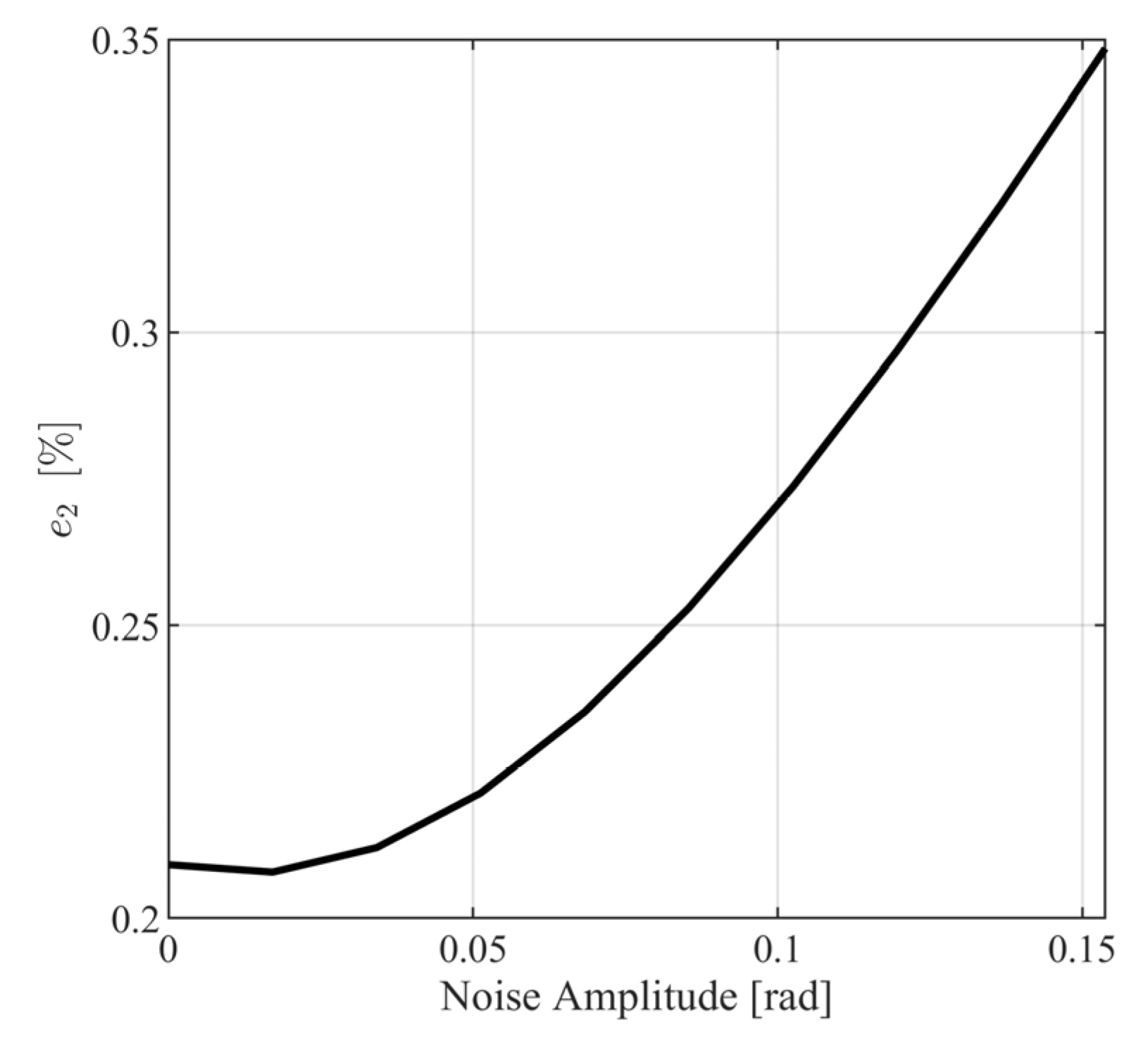
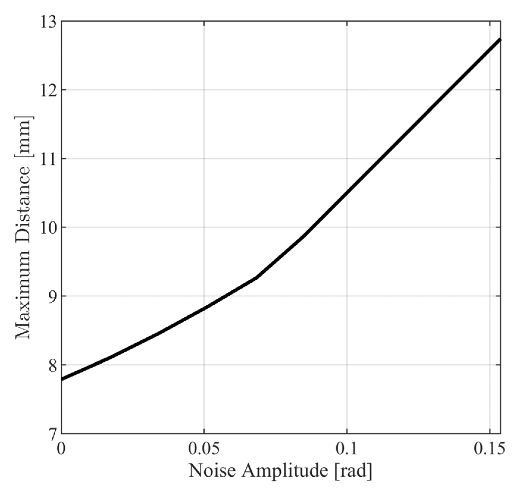
6.2. Performance of the Controller under Modeling Errors and Measurement Noise

In order to demonstrate the stability properties of the linear approximant closed loop system (115), consider the model and controller parameters presented in Section 6.1. Through applying a series of computational experiments, in Figure 16, the area of uncertainties where the polynomial in (116) is stable is presented.

Figure 16. Stability region of the closed loop system with respect to uncertainties.

In particular, the uncertain model parameters will be selected to be of the form $\delta B_m=p_{B_m}{B}_{m,0}$, $\delta R_m=p_{R_m}{R}_{m,0}$, and $\delta L_r=p_{L_r}{L}_{r,0}$ where $p_{B_m}\in \left(-1,2\right]$, $p_{R_m}\in \left(-1,2\right]$, and $p_{L_r}\in \left(-1,2\right]$. From Figure 16, it can readily be verified that $p_c\left(s,z\right)$ remains stable for a wide range of uncertainties and includes all positive values of them. For the negative values of $p_{B_m}$, $p_{R_m}$, and $p_{L_r}$, it can be observed that the linear approximant of the closed loop system may not be stable. Nevertheless, it is important to keep in mind that during motor operation, electrical resistance and viscous torque constant tend to increase with respect to time. Thus, from Figure 16, it can be observed that if the electrical resistance and viscous torque constant are increased from their nominal values, then the linear approximant closed loop system remains stable, independently of the motor inductance.

In order to demonstrate the performance of the proposed control scheme, in the presence of measurement noise and modeling errors, a series of computational experiments will be performed. First, the influence of measurement noise will be examined. The measurement noise is considered to be a high frequency low amplitude signal of a random type. For simulation purposes, the noise is produced as a continuous time waveform, derived using a pseudo-random number generator that produces a zero-mean random discrete time signal of unity amplitude. The random discrete time signal will be fed to a continuous time transfer function, considering a zero-order-hold in the input. In order to study the influence of the amplitude of the noise, the initially generated signal will be multiplied by an appropriate positive scaling factor.

In what follows, the filter transfer function is selected to be of the form

$$H_f\left(s\right)=\frac{1}{\left(T_{f,1}s+1\right)\left(T_{f,2}s+1\right)\left(T_{f,3}s+1\right)},$$

(120)

where $T_{f,1}=0.001$, $T_{f,1}=0.002$, and $T_{f,1}=0.003$. The heading angle measurement noise signal will be considered to be of the form

$${\psi }_{n,5}\left(t\right)={\lambda }_n{f}_n\left(t\right),$$

(121)

where $f_n\left(t\right)$ is a base waveform (see Figure 17 for $t\in \left[0, 0.6\right]\left[\sec \right]$) and ${\lambda }_n\in \left[0,+\infty \right)$ is the respective scaling factor.

Figure 17. Base orientation angle measurement noise signal $f_n\left(t\right)$.

The second noise signal ${\psi }_{n,6}\left(t\right)$, although, as already mentioned in Section 2, it is generally not related to ${\psi }_{n,5}\left(t\right)$, for simulation purposes, it will be assumed that ${\psi }_{n,6}\left(t\right)={\psi }_{n,5}^{\left(1\right)}\left(t\right)$, where the time derivative of ${\psi }_{n,5}\left(t\right)$ will be computed simply by using the filter

$${\overline{H}}_f\left(s\right)=\frac{s}{\left(T_{f,1}s+1\right)\left(T_{f,2}s+1\right)\left(T_{f,3}s+1\right)}.$$

(122)

Τhe signal $f_n\left(t\right)$ and for $t\in \left[0,0.6\right]$ will have the following indicative form.

The internal controller achieves decoupling between the velocity of the vehicle and the angular velocity of the mobile robot. The outer loop controller feeds the command to the angular velocity. Clearly, the orientation and angular velocity measurement noises only affect the second performance variable, namely the orientation angle. To quantitatively evaluate the performance of the control scheme in the presence of measurement noise, the simulation experiments, performed in Section 5, will be performed for various values of ${\lambda }_n\in \left[0, 0.08\right]$. The model response and the closed loop response for the second performance are denoted by $y_{2,m}\left(t\right)$ and $y_{2,n}\left(t\right)$, respectively. Through a series of computational experiments, the difference between $y_{2,m}\left(t\right)$ and $y_{2,n}\left(t\right)$ will be quantified using appropriate signal norms. To this end, define norm metrics as

$$e_{\infty }=\frac{{‖y_{2,m}\left(t\right)-y_{2,n}\left(t\right)‖}_{\infty }}{{‖y_{2,m}\left(t\right)-y_{2,n}\left(0-\right)‖}_{\infty }}\times 100\%,$$

(123)

$$e_2=\frac{{‖y_{2,m}\left(t\right)-y_{2,n}\left(t\right)‖}_2}{{‖y_{2,m}\left(t\right)-y_{2,n}\left(0-\right)‖}_2}\times 100\%,$$

(124)

where ${‖f\left(t\right)‖}_{\infty }=\underset{t\in \left[0,T_{\max }\right]}{\sup }\left|f\left(t\right)\right|$ and ${‖f\left(t\right)‖}_2^2={\displaystyle \underset{0-}{\overset{T_{\max }}{\int }}f{\left(t\right)}^{2}dt}$. In Figure 18 and Figure 19, the metrics in (123) and (124) are presented for different values of ${\lambda }_n$. From Figure 18 and Figure 19, it is observed that the closed loop system behaves satisfactorily for a wide range of measurement noise amplitudes with norm metrics, being smaller than $0.7\%$ for $e_{\infty }$ and $0.36\%$ for $e_2$. Additionally, it can be observed that the maximum distance between the model response path and the noisy response path (see Figure 20) is smaller than $14\left[\mathrm{mm}\right]$.

Figure 18. Infinity norm metric $e_{\infty }$ for various values of ${\lambda }_n$.

Figure 19. Infinity norm metric $e_2$ for various values of ${\lambda }_n$.

Figure 20. Maximum path distance for various values of ${\lambda }_n$.

To demonstrate the efficiency of the proposed control scheme in the presence of disturbances and faults, a computational experiment, being similar to those for the case of measurement noise, will be executed. For demonstration purposes, the disturbances and faults signals will be considered to be of the form

$${\xi }_j\left(t\right)={\mu }_j{f}_{m,j}\left(t\right) ; j=1,\dots ,4$$

(125)

where $f_{m,j}\left(t\right)$ ($j=1,\dots ,4$) are continuous time random type signals of unity amplitude, representing base waveforms, and ${\mu }_j\in \left[0,+\infty \right)$ are appropriate scaling factors. The generation of $f_{m,j}\left(t\right)$ is similar to that used for the generation of the measurement noise signal. The continuous signal reconstruction filter will also be of the form (120). Note that the random discrete time signal generators are different for each $f_{m,j}\left(t\right)$, thus producing independent base waveforms. Let $y_{1,e}\left(t\right)$ and $y_{2,e}\left(t\right)$ be the performance output responses in the presence of modelling errors. Let $y_1\left(t\right)$ and $y_2\left(t\right)$ be the performance output responses without modelling errors and measurement noise. Let

$${\gamma }_{k,\infty }=\frac{{‖y_{k,e}\left(t\right)-y_k\left(t\right)‖}_{\infty }}{{‖y_k\left(t\right)-y_k\left(0-\right)‖}_{\infty }}\times 100\% ; k=1,2$$

(126)

$${\gamma }_{k,2}=\frac{{‖y_{k,e}\left(t\right)-y_k\left(t\right)‖}_2}{{‖y_k\left(t\right)-y_k\left(0-\right)‖}_2}\times 100\% ; k=1,2$$

(127)

To quantitatively evaluate the performance of the control scheme in the presence of modelling errors, the same simulation experiment performed in Section 6.1 will be repeated for various values of ${\mu }_j$ ($j=1,\dots ,4$). Defining the four-dimensional radius,

$$\rho =\sqrt{{\displaystyle \sum _{j=1}^4{\mu }_j^2}}.$$

(128)

Applying a series of computational experiments for noise amplitudes up to ${10}^{-2}$, it can be verified that ${\gamma }_{1,\infty }$, ${\gamma }_{2,\infty }$, ${\gamma }_{1,2}$, and ${\gamma }_{2,2}$ are smaller than 25% for all $\rho$, being smaller than $0.0013$, $0.044$, $0.0017$, and $0.1$, respectively. These values, being four-dimensional radii, correspond to the noise amplitudes in Table 2. Using the simulation data as well as Table 2, it can be verified that, depending on the combinations of the noise amplitudes, different radii may be achieved.

Table 2. Maximum noise amplitudes satisfying performance criterion.

	${\gamma }_{1,\infty }$	${\gamma }_{2,\infty }$	${\gamma }_{1,2}$	${\gamma }_{2,2}$
${\mu }_1$	$0.000075$	$0.088755$	$0.000199$	$0.1$
${\mu }_2$	$0.000083$	$0.060664$	$0.000618$	$0.1$
${\mu }_3$	$0.00098$	$0.076619$	$0.000441$	$0.1$
${\mu }_4$	$0.000228$	$0.086698$	$0.000043$	$0.1$

7. Conclusions

In this study, the development of a nonlinear controller regulating the velocity and orientation angle of a differential drive mobile robot has been investigated. The system model being in nonlinear state space form has incorporated unknown disturbances and actuator faults. Using this nonlinear system, the input/output relationship has been established. A nonlinear controller consisting of two stages, which used measurable output feedback, has been developed. This controller has been segmented into internal and external control elements, a structure that is conducive to implementation on suitable experimental platforms. The controller has been designed to linearize the closed-loop system and control the robot’s velocity and angular velocity independently, utilizing a nonlinear PD controller that used real-time measurements of the wheels’ angular velocities and accelerations. The external controller, focusing on the regulation of the vehicle’s orientation angle, has employed a linear delayed PD feedback mechanism that processed measurements of the vehicle’s orientation angle and angular velocity, presumed to be wirelessly transmitted to the controller. Analytic formulas of the outer loop’s free controller parameters have been determined to ensure system stability, despite wireless transmission delays, and to achieve asymptotic command following to orientation angle commands. To compensate measurement noise and modelling errors, a metaheuristic algorithm has been proposed for adjusting the remaining controller parameters. The effectiveness of this control strategy has been verified through a series of computational experiments, which revealed satisfactory performances.

Future perspectives of the present work include (a) the investigation of the problem with delay-dependent controllers (indicatively see [50]), (b) the application of the proposed approach to robotic vehicles carrying manipulators that grasp known and unknown loads (indicatively see [51]), (c) the application of the proposed approach robotic vehicles moving in semi-structured and unstructured environments (indicatively see [52,53,54]), and (d) the application of the proposed approach to multi-transmission delay cases (indicatively see [55,56,57]). The experimental validation of the theoretical and simulation results is currently underway.

Appendix A.1. Elements of $\Gamma \left(x,u,\xi \right)$

$$\begin{gathered} {\gamma }_1\left(x,u,\xi \right)=\frac{1}{4b_W^2{\nu }_1{\nu }_2}\left\{-d_W{m}_P{r}_W^3\left(b_W^2{\nu }_1-{\nu }_2\right)x_1{\left(t\right)}^2+4B_m{b}_W^2\left(b_W^2{\nu }_1-{\nu }_2\right)x_2\left(t\right)+\right. \\ {d}_W{m}_P{r}_W^3\left(b_W^2{\nu }_1+{\nu }_2\right)x_2{\left(t\right)}^2-2x_1\left(t\right)\left[2B_m{b}_W^2\left(b_W^2{\nu }_1+{\nu }_2\right)+d_W{m}_P{r}_W^3{\nu }_2{x}_2\left(t\right)\right]+ \\ \left.4b_W^2\left[\left(b_W^2{\nu }_1+{\nu }_2\right)\left(K_m{r}_m{x}_4\left(t\right)+{\xi }_1\left(t\right)\right)-\left(b_W^2{\nu }_1-{\nu }_2\right)\left(K_m{r}_m{x}_5\left(t\right)+{\xi }_2\left(t\right)\right)\right]\right\} \\ {\gamma }_2\left(x,u,\xi \right)=\frac{1}{4b_W^2{\nu }_1{\nu }_2}\left\{d_W{m}_P{r}_W^3\left(b_W^2{\nu }_1+{\nu }_2\right)x_1{\left(t\right)}^2-4B_m{b}_W^2\left(b_W^2{\nu }_1+{\nu }_2\right)x_2\left(t\right)-\right. \\ -d_W{m}_P{r}_W^3\left(b_W^2{\nu }_1-{\nu }_2\right)x_2{\left(t\right)}^2+x_1\left(t\right)\left(4B_m{b}_W^4{\nu }_1-4B_m{b}_W^2{\nu }_2-2d_W{m}_P{r}_W^3{\nu }_2{x}_2\left(t\right)\right)+ \\ \left.4b_W^2\left[\left(b_W^2{\nu }_1+{\nu }_2\right)\left(K_m{r}_m{x}_5\left(t\right)+{\xi }_2\left(t\right)\right)-\left(b_W^2{\nu }_1-{\nu }_2\right)\left(K_m{r}_m{x}_4\left(t\right)+{\xi }_1\left(t\right)\right)\right]\right\}, \\ {\gamma }_3\left(x,u,\xi \right)=\frac{r_W}{2b_W}\left(x_2\left(t\right)-x_1\left(t\right)\right), \\ {\gamma }_4\left(x,u,\xi \right)=-\frac{K_b{r}_m}{L_r}{x}_1\left(t\right)-\frac{R_m}{L_r}{x}_4\left(t\right)+\frac{1}{L_r}\left(u_1\left(t\right)+{\xi }_3\left(t\right)\right), \\ {\gamma }_5\left(x,u,\xi \right)=-\frac{K_b{r}_m{x}_2}{L_r}\left(t\right)-\frac{R_m}{L_r}{x}_5\left(t\right)+\frac{1}{L_r}\left(u_2\left(t\right)+{\xi }_4\left(t\right)\right), \end{gathered}$$

Appendix A.2. Closed Loop Linear Approximant System Matrix Elements

$${\left({\tilde{e}}_0\right)}_{1,1}=J_{W,y}+\frac{r_W^2}{4b_W^2}\left[J_P+2J_{W,z}+d_W^2{m}_P+b_W^2\left(m_P+4m_W\right)\right],$$

$${\left({\tilde{e}}_0\right)}_{1,2}=\frac{r_W^2}{4b_W^2}\left[\left(b_W^2-d_W^2\right)m_P-J_P-2J_{W,z}\right],$$

$${\left({\tilde{e}}_0\right)}_{1,3}=-\frac{d_W{m}_P{r}_W^2{\overline{x}}_2}{2b_W}, {\left({\tilde{e}}_0\right)}_{2,1}={\left(e_0\right)}_{1,2}, {\left({\tilde{e}}_0\right)}_{2,2}={\left(e_0\right)}_{1,1},$$

$${\left({\tilde{e}}_0\right)}_{2,3}=\frac{2\left({\left(e_0\right)}_{1,2}-{\left(e_0\right)}_{1,1}\right)\left({\left(e_0\right)}_{4,2}-{\left(e_0\right)}_{5,1}\right)\left(1+{\beta }^2\right){\tan }^{-1}{\left(\nu \right)}^2}{3{\left(a_0\right)}_{3,1}^2{\left(e_1\right)}_{4,3}\left({\beta }^2-1\right){\left({\tau }^{*}\right)}^2}-{\left(e_0\right)}_{1,3}, {\left({\tilde{e}}_0\right)}_{3,3}=1,$$

$${\left({\tilde{e}}_0\right)}_{4,1}=-\left\{d_W{L}_{r,0}{m}_P{r}_W^3{\overline{x}}_2\left({\beta }^2-1\right){\tau }^{*}+\right.$$

$$\left(4B_{m,0}{b}_W^2{L}_{r,0}+\left(J_P+2J_{W,z}+d_W^2{m}_P\right)r_W^2\left(R_{m,0}-L_{r,0}{\mu }_0\right)+b_W^2\left\{4J_{W,y}{R}_{m,0}-2J_{W,y}{L}_{r,0}\left({\lambda }_{1,1}+{\mu }_0\right)+\right.\right.$$

$$\left.\left.r_W^2\left[4m_W{R}_{m,0}+m_P\left(R_{m,0}-L_{r,0}{\lambda }_{1,1}\right)-2L_{r,0}{m}_W\left({\lambda }_{1,1}+{\mu }_0\right)\right]\right\}\right)\left({\beta }^2-1\right){\tau }^{*}+$$

$$\left.4L_{r,0}\left[\left(J_P+2J_{W,z}+d_W^2{m}_P\right)r_W^2+2b_W^2\left(J_{W,y}+m_W{r}_W^2\right)\right]\beta {\tan }^{-1}\left(\beta \right)\right\}/$$

$$\left[4b_W^2{K}_m{r}_m\left(L_{r,0}+\delta L_r\right)\left({\beta }^2-1\right){\tau }^{*}\right],$$

$${\left({\tilde{e}}_0\right)}_{4,2}=\left(\left\{\left[J_P+2J_{W,z}+\left(d_W^2-b_W^2\right)m_P\right]R_{m,0}{r}_W^2-d_W{L}_{r,0}{m}_P{r}_W^3{\overline{x}}_1+\right.\right.$$

$$2d_W{L}_{r,0}{m}_P{r}_W^3{\overline{x}}_2+2b_W^2{J}_{W,y}{L}_{r,0}{\lambda }_{1,1}+b_W^2{L}_{r,0}{m}_P{r}_W^2{\lambda }_{1,1}+2b_W^2{L}_{r,0}{m}_W{r}_W^2{\lambda }_{1,1}-$$

$$\left.L_{r,0}\left[\left(J_P+2J_{W,z}+d_W^2{m}_P\right)r_W^2+2b_W^2\left(J_{W,y}+m_W{r}_W^2\right)\right]{\mu }_0\right\}\left({\beta }^2-1\right){\tau }^{*}+$$

$$\left.4L_{r,0}\left[\left(J_P+2J_{W,z}+d_W^2{m}_P\right)r_W^2+2b_W^2\left(J_{W,y}+m_W{r}_W^2\right)\right]\beta {\tan }^{-1}\left(\beta \right)\right)/$$

$$\left[4b_W^2{K}_m{r}_m\left(L_{r,0}+\delta L_r\right)\left({\beta }^2-1\right){\tau }^{*}\right], {\left({\tilde{e}}_0\right)}_{4,4}=1$$

$${\left({\tilde{e}}_0\right)}_{5,1}=\left(\left\{\left[J_P+2J_{W,z}+\left(d_W^2-b_W^2\right)m_P\right]R_{m,0}{r}_W^2+2d_W{L}_{r,0}{m}_P{r}_W^3{\overline{x}}_1-\right.\right.$$

$$d_W{L}_{r,0}{m}_P{r}_W^3{\overline{x}}_2+2b_W^2{J}_{W,y}{L}_{r,0}{\lambda }_{1,1}+b_W^2{L}_{r,0}{m}_P{r}_W^2{\lambda }_{1,1}+2b_W^2{L}_{r,0}{m}_W{r}_W^2{\lambda }_{1,1}-$$

$$\left.L_{r,0}\left[\left(J_P+2J_{W,z}+d_W^2{m}_P\right)r_W^2+2b_W^2\left(J_{W,y}+m_W{r}_W^2\right)\right]{\mu }_0\right\}\left({\beta }^2-1\right){\tau }^{*}+$$

$$\left.4L_{r,0}\left[\left(J_P+2J_{W,z}+d_W^2{m}_P\right)r_W^2+2b_W^2\left(J_{W,y}+m_W{r}_W^2\right)\right]\beta {\tan }^{-1}\left(\beta \right)\right)/$$

$$\left[4b_W^2{K}_m{r}_m\left(L_{r,0}+\delta L_r\right)\left({\beta }^2-1\right){\tau }^{*}\right], {\left({\tilde{e}}_0\right)}_{5,2}=\left(3{\left(e_0\right)}_{4,1}+{\left(e_0\right)}_{4,2}-{\left(e_0\right)}_{5,1}\right)/3, {\left({\tilde{e}}_0\right)}_{5,5}=1,$$

$${\left({\tilde{e}}_1\right)}_{4,3}=\frac{2L_{r,0}\left[\left(J_P+2J_{W,z}+d_W^2{m}_P\right)r_W^2+2b_W^2\left(J_{W,y}+m_W{r}_W^2\right)\right]\left(1+{\beta }^2\right){\tan }^{-1}{\left(v\right)}^2}{b_W{K}_m{r}_m{r}_W\left(L_{r,0}+\delta L_r\right)\left({\beta }^2-1\right){\left({\tau }^{*}\right)}^2}$$

$${\left({\tilde{e}}_1\right)}_{5,3}={\left({\tilde{e}}_1\right)}_{4,3}, {\left({\tilde{a}}_0\right)}_{1,1}=-\left(B_{m,0}+\delta B_m\right), {\left({\tilde{a}}_0\right)}_{1,4}=K_m{r}_m, {\left({\tilde{a}}_0\right)}_{2,2}={\left(a_0\right)}_{1,1}, {\left({\tilde{a}}_0\right)}_{2,5}={\left(a_0\right)}_{1,4},$$

$${\left({\tilde{a}}_0\right)}_{3,1}=-\frac{r_W}{2b_W}, {\left({\tilde{a}}_0\right)}_{3,2}=-{\left({\tilde{a}}_0\right)}_{3,1},$$

$${\left({\tilde{a}}_0\right)}_{4,1}=\left(\left\{4B_{m,0}{b}_W^2{R}_{m,0}+d_W{m}_P{R}_{m,0}{r}_W^3{\overline{x}}_2-b_W^2{L}_{r,0}{\lambda }_{0,1}\left[2J_{W,y}+\left(m_P+2m_W\right)r_W^2\right]\right\}\left({\beta }^2-1\right){\tau }^{*}+\right.$$

$$\left.4L_{r,0}\left[\left(J_P+2J_{W,z}+d_W^2{m}_P\right)r_W^2+2b_W^2\left(J_{W,y}+m_W{r}_W^2\right)\right]{\mu }_0\beta {\tan }^{-1}\left(\beta \right)\right)/$$

$$\left[4b_W^2{K}_m{r}_m\left(L_{r,0}+\delta L_r\right)\left({\beta }^2-1\right){\tau }^{*}\right],$$

$${\left({\tilde{a}}_0\right)}_{4,2}=\left(\left\{d_W{m}_P{R}_{m,0}{r}_W^3\left({\overline{x}}_1-2{\overline{x}}_2\right)-b_W^2{L}_{r,0}\left[2J_{W,y}+\left(m_P+2m_W\right)r_W^2\right]{\lambda }_{0,1}\right\}\left({\beta }^2-1\right){\tau }^{*}-\right.$$

$$\left.4L_{r,0}\left[\left(J_P+2J_{W,z}+d_W^2{m}_P\right)r_W^2+2b_W^2\left(J_{W,y}+m_W{r}_W^2\right)\right]{\mu }_0\beta {\tan }^{-1}\left(\beta \right)\right)/$$

$$\left[4b_W^2{K}_m{r}_m\left(L_{r,0}+\delta L_r\right)\left({\beta }^2-1\right){\tau }^{*}\right], {\left({\tilde{a}}_0\right)}_{4,4}=-\frac{R_{m,0}+\delta R_m}{L_{r,0}+\delta L_r},$$

$${\left({\tilde{a}}_0\right)}_{5,1}=\left(\left\{d_W{m}_P{R}_{m,0}{r}_W^3\left(2{\overline{x}}_1-{\overline{x}}_2\right)+b_W^2{L}_{r,0}\left[2J_{W,y}+\left(m_P+2m_W\right)r_W^2\right]{\lambda }_{0,1}\right\}\left({\beta }^2-1\right){\tau }^{*}+\right.$$

$$\left.4L_{r,0}\left[\left(J_P+2J_{W,z}+d_W^2{m}_P\right)r_W^2+2b_W^2\left(J_{W,y}+m_W{r}_W^2\right)\right]{\mu }_0\beta {\tan }^{-1}\left(\beta \right)\right)/$$

$$\left[4b_W^2{K}_m{r}_m\left(L_{r,0}+\delta L_r\right)\left(1-{\beta }^2\right){\tau }^{*}\right], {\left({\tilde{a}}_0\right)}_{5,2}=\left(3{\left(a_0\right)}_{4,1}+{\left(a_0\right)}_{4,2}-{\left(a_0\right)}_{5,1}\right)/3, {\left({\tilde{a}}_0\right)}_{5,5}={\left(a_0\right)}_{4,4}$$

$${\left({\tilde{a}}_1\right)}_{4,3}=\frac{2L_{r,0}\left[\left(J_P+2J_{W,z}+d_W^2{m}_P\right)r_W^2+2b_W^2\left(J_{W,y}+m_W{r}_W^2\right)\right]{\mu }_0\left(1+{\beta }^2\right){\tan }^{-1}{\left(\beta \right)}^2}{b_W{K}_m{r}_m{r}_W\left(L_{r,0}+\delta L_r\right)\left(1-{\beta }^2\right){\left({\tau }^{*}\right)}^2},$$

$${\left({\tilde{a}}_1\right)}_{5,3}=-{\left({\tilde{a}}_1\right)}_{4,3}, {\left({\tilde{b}}_0\right)}_{4,1}=\frac{L_{r,0}{\lambda }_{0,1}\left[2J_{W,y}+\left(m_P+2m_W\right)r_W^2\right]}{2K_m{r}_m{r}_W\left(L_{r,0}+\delta L_r\right)}, {\left({\tilde{b}}_0\right)}_{5,1}={\left({\tilde{b}}_0\right)}_{4,1},$$

$${\left({\tilde{b}}_0\right)}_{4,2}=\frac{2L_{r,0}\left[\left(J_P+2J_{W,z}+d_W^2{m}_P\right)r_W^2+2b_W^2\left(J_{W,y}+m_W{r}_W^2\right)\right]{\mu }_0\left(1+{\beta }^2\right){\tan }^{-1}{\left(\beta \right)}^2}{b_W{K}_m{r}_m{r}_W\left(L_{r,0}+\delta L_r\right)\left({\beta }^2-1\right){\left({\tau }^{*}\right)}^2},$$

$${\left({\tilde{b}}_0\right)}_{5,2}=-{\left({\tilde{b}}_0\right)}_{4,2}.$$

Appendix A.3. Closed Loop Linear Approximant Characteristic Polynomial Coefficients

$${\alpha }_1=\frac{2\left(B_{m,0}+\delta B_m\right)\delta L_r+2J_{W,y}\delta R_m+\left(m_P+2m_W\right)r_W^2\delta R_m+L_{r,0}\left[2\delta B_m+2J_{W,y}{\lambda }_{1,1}+\left(m_P+2m_W\right)r_W^2{\lambda }_{1,1}\right]}{\left(2J_{W,y}+\left(m_P+2m_W\right)r_W^2\right)\left(L_{r,0}+\delta L_r\right)},$$

$${\alpha }_0=\frac{2R_{m,0}\delta B_m+2\left(B_{m,0}+\delta B_m\right)\delta R_m}{\left[2J_{W,y}+\left(m_P+2m_W\right)r_W^2\right]\left(L_{r,0}+\delta L_r\right)}+\frac{L_{r,0}{\lambda }_{0,1}}{\left(L_{r,0}+\delta L_r\right)},$$

$${\beta }_{2,0}={\left(L_{r,0}+\delta L_r\right)}^{-1}\left[\left(2b_W^2\left\{2R_{m,0}\delta B_m+2\left(B_{m,0}+\delta B_m\right)\delta R_m+L_{r,0}\left[2J_{W,y}+\left(m_P+2m_W\right)r_W^2\right]{\lambda }_{0,1}\right\}\right.\right.$$

$$\left\{\left(B_{m,0}+\delta B_m\right)\delta L_r+\left(J_{W,y}+m_W{r}_W^2\right)\delta R_m+L_{r,0}\left[\delta B_m+\left(J_{W,y}+m_W{r}_W^2\right){\mu }_0\right]\right\}+$$

$$r_W^2\left(\left(J_P+2J_{W,z}\right)\left\{2R_{m,0}\delta B_m+2\left(B_{m,0}+\delta B_m\right)\delta R_m+L_{r,0}\left[2J_{W,y}+\left(m_P+2m_W\right)r_W^2\right]{\lambda }_{0,1}\right\}\left(\delta R_m+L_{r,0}{\mu }_0\right)+\right.$$

$$d_W{m}_P\left(L_{r,0}\left[2J_{W,y}+\left(m_P+2m_W\right)r_W^2\right]v^{*}\delta L_r{\lambda }_{0,1}+\right.$$

$$\left.\left.\left.d_W\left\{2R_{m,0}\delta B_m+2\left(B_{m,0}+\delta B_m\right)\delta R_m+L_{r,0}\left[2J_{W,y}+\left(m_P+2m_W\right)r_W^2\right]{\lambda }_{0,1}\right\}\left(\delta R_m+L_{r,0}{\mu }_0\right)\right)\right)\right)/$$

$$\left.4L_{r,0}\beta {\tan }^{-1}\left(\beta \right){\left[\left(1-{\beta }^2\right){\tau }^{*}\right]}^{-1}\right],$$

$${\beta }_{1,0}=\left\{\left[\left(4{\left[b_W{R}_{m,0}\delta B_m+b_W\left(B_{m,0}+\delta B_m\right)\delta R_m\right]}^2+L_{r,0}\left[2J_{W,y}+\left(m_P+2m_W\right)r_W^2\right]\right.\times \right.\right.$$

$$\left.\left\{d_W{m}_P{r}_W^2{v}^{*}\delta R_m+2b_W^2\left[R_{m,0}\delta B_m+\left(B_{m,0}+\delta B_m\right)\delta R_m\right]\right\}{\lambda }_{0,1}\right)/$$

$$\left(\left[\left(J_P+2J_{W,z}+d_W^2{m}_P\right)r_W^2+2b_W^2\left(J_{W,y}+m_W{r}_W^2\right)\right]\times \right.$$

$$\left.\left.\left\{2R_{m,0}\delta B_m+2\left(B_{m,0}+\delta B_m\right)\delta R_m+L_{r,0}\left[2J_{W,y}+\left(m_P+2m_W\right)r_W^2\right]{\lambda }_{0,1}\right\}\right)\right]+$$

$$\left.4L_{r,0}{\mu }_0\beta {\tan }^{-1}\left(\beta \right)/\left[\left(1-{\beta }^2\right){\tau }^{*}\right]\right\}/\left(L_{r,0}+\delta L_r\right),$$

$${\beta }_{1,1}={\beta }_{0,1}/{\mu }_0, {\beta }_{0,1}=\frac{4L_{r,0}{\mu }_0\left(1+{\beta }^2\right){\tan }^{-1}{\left(\beta \right)}^2}{\left(L_{r,0}+\delta L_r\right)\left(1-{\beta }^2\right){\left({\tau }^{*}\right)}^2}$$

References

- Cobos Torres, E.O.; Konduri, S.; Pagilla, P.R. Study of wheel slip and traction forces in differential drive robots and slip avoidance control strategy. In Proceedings of the 2014 American Control Conference (ACC), Portland, OR, USA, 4–6 June 2014; pp. 3231–3236. [Google Scholar]
- Cobos Torres, E.O. Traction Modeling and Control of a Differential Drive Mobile Robot to Avoid Wheel Slip. Master’s Thesis, Oklahoma State University, Stillwater, OK, USA, 2013. [Google Scholar]
- Dhaouadi, R.; Hatab, A.A. Dynamic Modelling of Differential-Drive Mobile Robots using Lagrange and Newton-Euler Methodologies: A Unified Framework. Adv. Robot. Autom. 2013, 2, 1–7. [Google Scholar]
- Anvari, I. Non-holonomic Differential Drive Mobile Robot Control & Design: Critical Dynamics and Coupling Constraints. Master’s Thesis, Arizona State University, Tempe, AZ, USA, 2013. [Google Scholar]
- Kouvakas, N.D.; Koumboulis, F.N.; Sigalas, J. Manoeuvring of Differential Drive Mobile Robots on Horizontal Plane through I/O Decoupling. In Proceedings of the 2022 IEEE 27th International Conference on Emerging Technologies and Factory Automation (ETFA), Stuttgart, Germany, 6–9 September 2022. [Google Scholar]
- Tzafestas, S.G. Mobile robot control and navigation: A global overview. J. Intell. Robot. Syst. 2018, 91, 35–58. [Google Scholar] [CrossRef]
- Rubio, F.; Valero, F.; Llopis-Albert, C. A review of mobile robots: Concepts, methods, theoretical framework, and applications. Int. J. Adv. Robot. Syst. 2019, 16, 1729881419839596. [Google Scholar] [CrossRef]
- Martins, O.O.; Adekunle, A.A.; Adejuyigbe, S.B.; Adeyemi, O.H.; Oluwole, A.; Arowolo, M.O. Wheeled Mobile Robot Path Planning and Path Tracking Controller Algorithms: A Review. J. Eng. Sci. Technol. Rev. 2020, 13, 152–164. [Google Scholar] [CrossRef]
- Kamel, M.A.; Zhang, Y. Developments and challenges in wheeled mobile robot control. In Proceedings of the 2014 International Conference on Intelligent Unmanned Systems (ICIUS 2014), Montreal, QC, Canada, 29 September–1 October 2014. [Google Scholar]
- Heikkinen, J.; Minav, T.; Stotckaia, A.D. Self-tuning parameter fuzzy PID controller for autonomous differential drive mobile robot. In Proceedings of the 2017 XX IEEE International Conference on Soft Computing and Measurements (SCM), St. Petersburg, Russia, 24–26 May 2017. [Google Scholar]
- Drosou, T.C.; Kouvakas, N.D.; Koumboulis, F.N.; Tzamtzi, M.P. A Mixed Analytic/Metaheuristic Dual Stage Control Scheme Toward I/O Decoupling for a Differential Drive Mobile Robot. In Proceedings of the Springer 1st International Conference on Frontiers of Artificial Intelligence, Ethics, and Multidisciplinary Applications, Athens, Greece, 25–26 September 2023. [Google Scholar]
- Hendzel, Z.; Szuster, M. Approximate Dynamic Programming in Robust Tracking Control of Wheeled Mobile Robot. Arch. Mech. Eng. 2009, LVI, 223–236. [Google Scholar] [CrossRef]
- Hendzel, Z.; Penar, P. Optimal Control of a Wheeled Robot. In Automation 2019: Progress in Automation, Robotics and Measurement Techniques; Szewczyk, R., Zieliński, C., Kaliczyńska, M., Eds.; Springer: Berlin/Heidelberg, Germany, 2020; pp. 473–481. [Google Scholar]
- Hendzel, Z.; Penar, P. Experimental verification of H∞ control with examples of the movement of a wheeled robot. Bull. Pol. Acad. Sci. Tech. Sci. 2021, 69, e139390. [Google Scholar] [CrossRef]
- Penar, P.; Hendzel, Z. Experimental Verification of the Differential Games and H∞ Theory in Tracking Control of a Wheeled Mobile Robot. J. Intell. Robot. Syst. 2022, 104, 61. [Google Scholar] [CrossRef]
- Recalde, L.F.; Guevara, B.S.; Cuzco, G.; Andaluz, V.H. Optimal Control Problem of a Differential Drive Robot. In Trends in Artificial Intelligence Theory and Applications. Artificial Intelligence Practices. IEA/AIE 2020; Fujita, H., Fournier-Viger, P., Ali, M., Sasaki, J., Eds.; Lecture Notes in Computer Science; Springer: Cham, Switzerland, 2020; Volume 12144. [Google Scholar]
- Bouzoualegh, S.; Guechi, E.-H.; Kelaiaia, R. Model Predictive Control of a Differential-Drive Mobile Robot. Acta Univ. Sapientiae Electr. Mech. Eng. 2018, 10, 20–41. [Google Scholar] [CrossRef]
- Sharma, K.R.; Honc, D.; Dušek, F. Predictive Control of Differential Drive Mobile Robot Considering Dynamics and Kinematics. In Proceedings of the 30th European Conference on Modelling and Simulation, Regensburg, Germany, 31 May–3 June 2016. [Google Scholar]
- Hendzel, Z.; Trojnacki, M. Adaptive Fuzzy Control of a Four-Wheeled Mobile Robot Subject to Wheel Slip. WSEAS Trans. Syst. 2023, 22, 602–612. [Google Scholar]
- Štefek, A.; Pham, V.T.; Krivanek, V.; Pham, K.L. Optimization of Fuzzy Logic Controller Used for a Differential Drive Wheeled Mobile Robot. Appl. Sci. 2021, 11, 6023. [Google Scholar] [CrossRef]
- Jardine, P.T.; Kogan, M.; Givigi, S.N.; Yousefi, S. Adaptive predictive control of a differential drive robot tuned with reinforcement learning. Int. J. Adapt. Control Signal Process. 2019, 33, 410–423. [Google Scholar] [CrossRef]
- Szuster, M.; Hendzel, Z. Intelligent Optimal Adaptive Control for Mechatronic Systems; Springer: Berlin/Heidelberg, Germany, 2018. [Google Scholar]
- Khooban, M.H. Design an intelligent proportional-derivative (PD) feedback linearization control for nonholonomic-wheeled mobile robot. J. Intell. Fuzzy Syst. 2014, 26, 1833–1843. [Google Scholar] [CrossRef]
- Koumboulis, F.N. On the Common Control Design of Robotic Manipulators Carrying Different Loads. In Advances in Service and Industrial Robotics, RAAD 2018, Mechanisms and Machine Science; Aspragathos, N., Koustoumpardis, P., Moulianitis, V., Eds.; Springer: Cham, Switzerland, 2019; Volume 67. [Google Scholar]
- Shojaei, K.; Shahri, A.M.; Tabibian, B. Design and Implementation of an Inverse Dynamics Controller for Uncertain Nonholonomic Robotic Systems. J. Intell. Robot. Syst. 2013, 71, 65–83. [Google Scholar] [CrossRef]
- Pedapati, P.K.; Pradhan, S.K.; Kumar, S. Kinematic Control of an Autonomous Ground Vehicle Using Inverse Dynamics Controller. In Advances in Smart Grid Automation and Industry 4.0; Lecture Notes in Electrical Engineering; Reddy, M.J.B., Mohanta, D.K., Kumar, D., Ghosh, D., Eds.; Springer: Singapore, 2021; Volume 693. [Google Scholar]
- Chwa, D. Tracking Control of Differential-Drive Wheeled Mobile Robots Using a Backstepping-Like Feedback Linearization. IEEE Trans. Syst. Man Cybern.—Part A Syst. Hum. 2010, 40, 1285–1295. [Google Scholar] [CrossRef]
- Tiriolo, C.; Franzè, G.; Lucia, W. A Receding Horizon Trajectory Tracking Strategy for Input-Constrained Differential-Drive Robots via Feedback Linearization. IEEE Trans. Control Syst. Technol. 2023, 31, 1460–1467. [Google Scholar] [CrossRef]
- Tiriolo, C.; Franzè, G.; Lucia, W. An Obstacle-Avoidance Receding Horizon Control Scheme for Constrained Differential-Drive Robot via Dynamic Feedback Linearization. In Proceedings of the 2023 American Control Conference (ACC), San Diego, CA, USA, 31 May–2 June 2023. [Google Scholar]
- Koumboulis, F.N.; Kouvakas, N.D.; Giannaris, G.L.; Vouyioukas, D. Independent motion control of a tower crane through wireless sensor and actuator networks. ISA Trans. 2016, 60, 312–320. [Google Scholar] [CrossRef] [PubMed]
- Kouvakas, N.D.; Koumboulis, F.N.; Drosou, T.C. On the Remote Control of Differential Drive Mobile Robots through Wireless Networks. In Proceedings of the 2022 IEEE 1st Industrial Electronics Society Annual On-Line Conference (ONCON), Kharagpur, India, 9–11 December 2022. [Google Scholar]
- Kotta, Ü.; Mullari, T. Realization of nonlinear systems described by input/output differential equations: Equivalence of different methods. In Proceedings of the 2003 European Control Conference (ECC), Cambridge, UK, 1–4 September 2003. [Google Scholar]
- Moog, C.H.; Zheng, Y.; Liu, P. Input-Output equivalence of Nonlinear Systems and their Realizations. In Proceedings of the IFAC 15th Trennial World Congress, Barcelona, Spain, 21–26 July 2002; pp. 265–270. [Google Scholar]
- Monteriù, A.; Asthana, P.; Valavanis, K.P.; Longhi, S. Real-Time Model-Based Fault Detection and Isolation for UGVs. J. Intell. Robot. Syst. 2009, 56, 425–439. [Google Scholar] [CrossRef]
- Myint, C.; Win, N.N. Position and Velocity Control for Two-Wheel Differential Drive Mobile Robot. Int. J. Sci. Eng. Technol. Res. 2016, 5, 2849–2855. [Google Scholar]
- Araki, N.; Sato, T.; Konishi, Y.; Ishigaki, H. Vehicle’s Orientation Measurement Method by Single-Camera Image Using Known-Shaped Planar Object. In Proceedings of the 2009 Fourth International Conference on Innovative Computing, Information and Control (ICICIC), Kaohsiung, Taiwan, 7–9 December 2009; pp. 193–196. [Google Scholar]
- Suzuki, T.; Kanada, T. Measurement of Vehicle Motion and Orientation using Optical Flow. In Proceedings of the 1999 IEEE/IEEJ/JSAI International Conference on Intelligent Transportation Systems, Tokyo, Japan, 5–8 October 1999; pp. 25–30. [Google Scholar]
- Van Breugel, F.; Kutz, J.N.; Brunton, B.W. Numerical Differentiation of Noisy Data: A Unifying Multi-Objective Optimization Framework. IEEE Access 2020, 8, 196865–196877. [Google Scholar] [CrossRef] [PubMed]
- Segovia, V.R.; Hägglund, T.; Aström, K.J. Measurement noise filtering for PID controllers. J. Process Control 2014, 24, 299–313. [Google Scholar] [CrossRef]
- Olgac, N.; Sipahi, R. An Exact Method for the Stability Analysis of Time-Delayed Linear Time-Invariant (LTI) Systems. IEEE Trans. Autom. Control 2002, 47, 793–797. [Google Scholar] [CrossRef]
- Ai, B.; Sentis, L.; Paine, N.; Han, S.; Mok, A.; Fok, C.-L. Stability and Performance Analysis of Time-Delayed Actuator Control Systems. J. Dyn. Syst. Meas. Control 2016, 138, 051005. [Google Scholar] [CrossRef]
- Paraskevopoulos, P.N. Modern Control Engineering; CRC Press: Boca Raton, FL, USA, 2002; Available online: https://www.taylorfrancis.com/books/mono/10.1201/9781315214573/modern-control-engineering-paraskevopoulos (accessed on 29 January 2024).
- Garcia-Sanz, M. Robust Control Engineering: Practical QFT Solutions; CRC Press: Boca Raton, FL, USA, 2017. [Google Scholar]
- Bhattacharyya, S.P.; Keel, L.H. Linear Multivariable Control Systems; Cambridge University Press: Cambridge, UK, 2022. [Google Scholar]
- Levine, W.S. (Ed.) The Control Handbook; CRC Press: Boca Raton, FL, USA, 2011; Available online: https://www.taylorfrancis.com/books/mono/10.1201/9781315218694/control-handbook-three-volume-set-william-levine (accessed on 29 January 2024).
- Doyle, J.D.; Francis, B.A.; Tannenbaum, A.R. Feedback Control Theory; Dover Publications: New York, NY, USA, 2009; Available online: https://books.google.co.jp/books?id=gD9nPgAACAAJ&lr&source=gbs_book_other_versions (accessed on 29 January 2024).
- Xia, H.; Zhao, P.; Li, L.; Wu, A.; Ma, G. A novel approach to H∞ control design for linear neutral time-delay systems. Math. Probl. Eng. 2013, 2013, 526017. [Google Scholar] [CrossRef]
- Rabeb, B.; Aicha, E.; Naceur, A.M. Fault diagnosis and fault-tolerant control design for neutral time delay system. Automatika 2023, 64, 422–430. [Google Scholar] [CrossRef]
- Fu, P.; Niculescu, S.-I.; Chen, J. Stability of linear neutral time-delay systems: Exact conditions via matrix pencil solutions. IEEE Trans. Autom. Control 2006, 51, 1063–1069. [Google Scholar] [CrossRef]
- Šika, Z.; Vyhlídal, T.; Neusser, Z. Two-dimensional delayed resonator for entire vibration absorption. J. Sound Vib. 2021, 500, 116010. [Google Scholar] [CrossRef]
- Jaramillo-Morales, M.F.; Dogru, S.; Marques, L. Generation of Energy Optimal Speed Profiles for a Differential Drive Mobile Robot with Payload on Straight Trajectories. In Proceedings of the 2020 IEEE International Symposium on Safety, Security, and Rescue Robotics (SSRR), Abu Dhabi, United Arab Emirates, 4–6 November 2020. [Google Scholar]
- Guastella, D.C.; Muscato, G. Learning-Based Methods of Perception and Navigation for Ground Vehicles in Unstructured Environments: A Review. Sensors 2021, 21, 73. [Google Scholar] [CrossRef] [PubMed]
- Mateus, D.; Avina, G.; Devy, M. Robot Visual Navigation in Semi-structured Outdoor Environments. In Proceedings of the 2005 IEEE International Conference on Robotics and Automation, Barcelona, Spain, 18–22 April 2005. [Google Scholar]
- LeSage, J.R.; Longoria, R.G. Mission Feasibility Assessment for Mobile Robotic Systems Operating in Stochastic Environments. J. Dyn. Syst. Meas. Control 2015, 137, 031009. [Google Scholar] [CrossRef]
- Yu, M.; Wang, L.; Chu, T.; Hao, F. Stabilization of Networked Control Systems with Data Packet Dropout and Transmission Delays: Continuous-Time Case. Eur. J. Control 2005, 11, 40–49. [Google Scholar] [CrossRef]
- Lian, F.-L.; Moyne, J.; Tilbury, D. Modelling and optimal controller design of networked control systems with multiple delays. Int. J. Control 2010, 76, 591–606. [Google Scholar] [CrossRef]
- Olgac, N.; Ergenc, A.F.; Sipahi, R. Delay Scheduling: A New Concept for Stabilization in Multiple Delay Systems. J. Vib. Control 2005, 11, 1159–1172. [Google Scholar] [CrossRef]
Disclaimer/Publisher’s Note: The statements, opinions and data contained in all publications are solely those of the individual author(s) and contributor(s) and not of MDPI and/or the editor(s). MDPI and/or the editor(s) disclaim responsibility for any injury to people or property resulting from any ideas, methods, instructions or products referred to in the content. |
© 2024 by the authors. Licensee MDPI, Basel, Switzerland. This article is an open access article distributed under the terms and conditions of the Creative Commons Attribution (CC BY) license (https://creativecommons.org/licenses/by/4.0/).