
Robust Nonlinear Model Predictive Control for the Trajectory Tracking of Skid-Steer Mobile Manipulators with Wheel–Ground Interactions

 ,
,  , ,
, ,  and
and 
Abstract
1. Introduction
2. Related Work
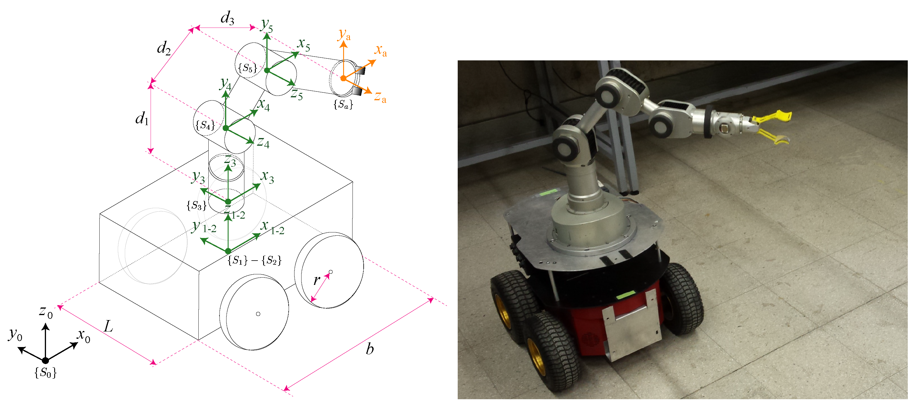
3. Dynamic Model of the Skid-Steer Mobile Manipulator
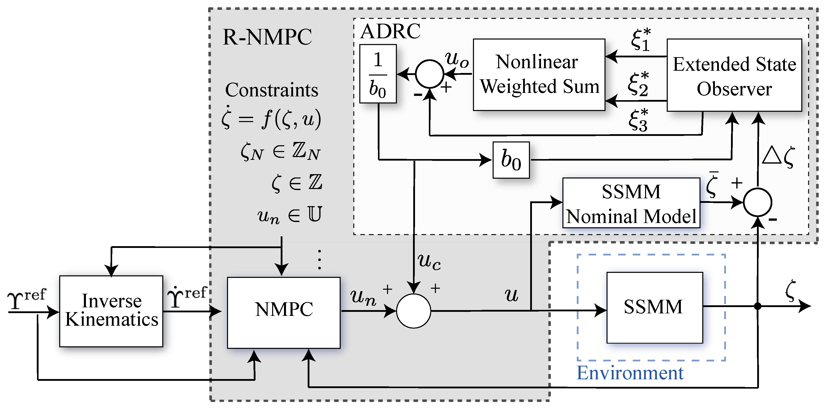
4. Nonlinear Model Predictive Control Strategy
5. Passivity-Based Robust Control Strategy
6. Experimental Tests and Results
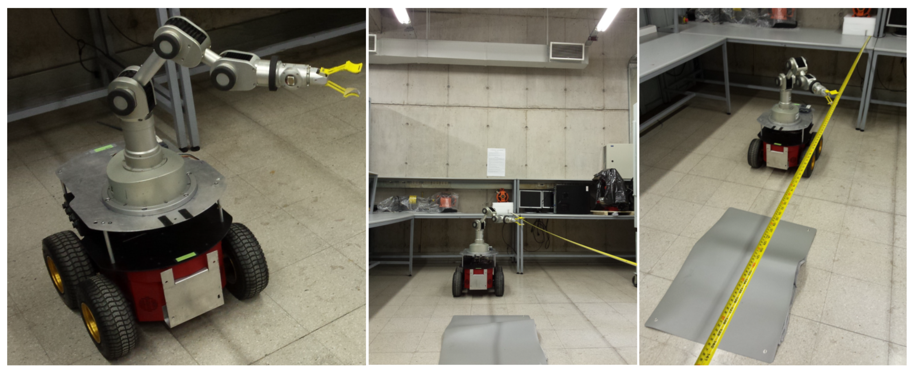
6.1. Experimental Setup
6.2. Simulation Test for Disturbance Rejection
6.3. Simulation Test Under Parameter Variations
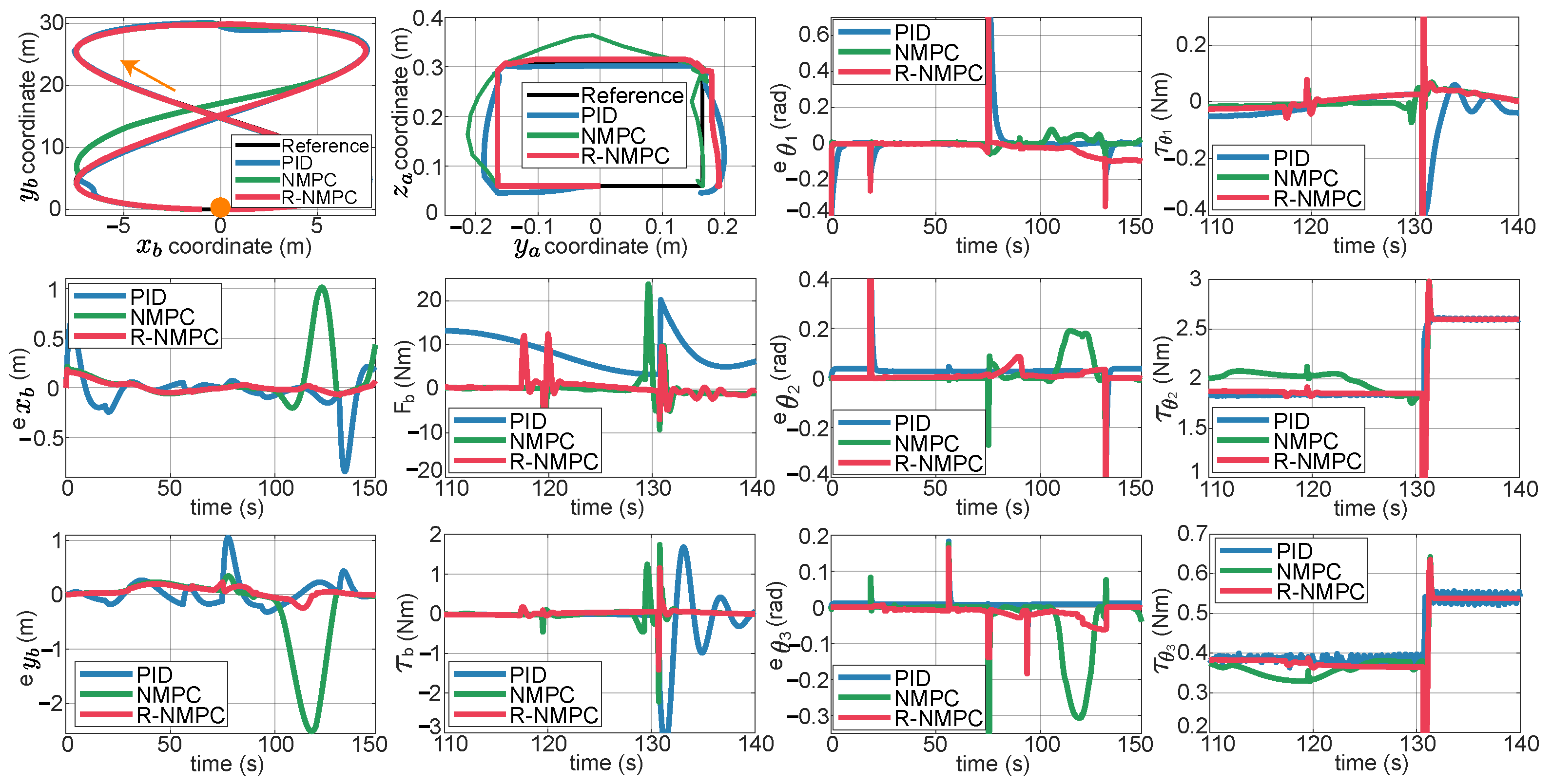
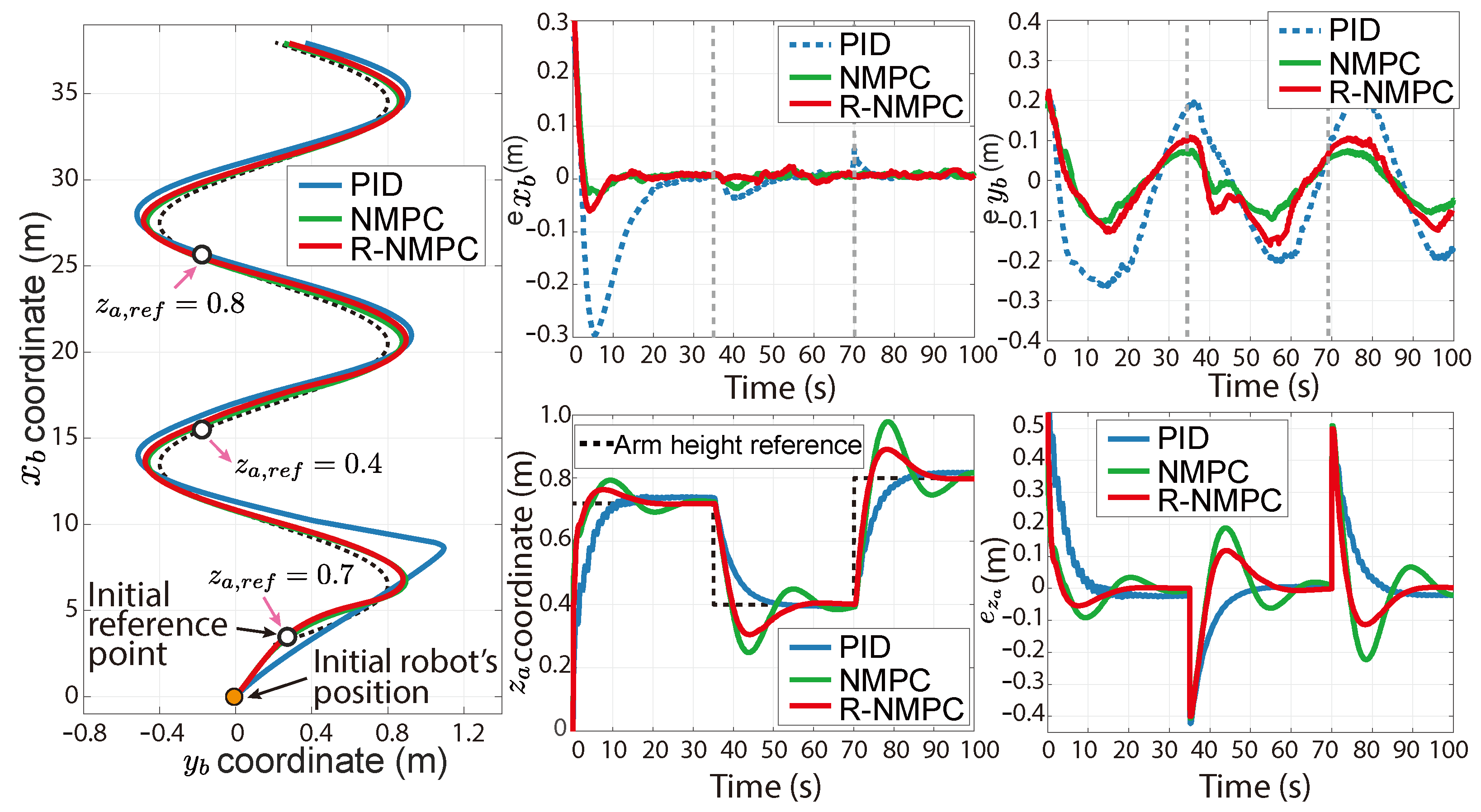
6.4. Field Test for Trajectory-Tracking Control
6.5. Field Test of Robustness Under Terrain Disturbances
7. Conclusions
Author Contributions
Funding
Data Availability Statement
Acknowledgments
Conflicts of Interest
Abbreviations
| MPC | Model Predictive Control |
| NMPC | Nonlinear Model Predictive Control |
| R-NMPC | Robust Nonlinear Model Predictive Control |
| PID | Proportional-Integral-Derivative |
| DoF | Degree of Freedom |
| SSMM | Skid-Steer Mobile Manipulator |
| ADRC | Active Disturbance Reject Control |
| SISO | Single-Input Single-Output |
| MIMO | Multiple-Input Multiple-Output |
| ESO | Extended State Observer |
| DH | Denavit–Hartenberg |
| N–E | Newton–Euler |
| OCP | Optimal Control Problem |
References
- Ghodsian, N.; Benfriha, K.; Olabi, A.; Gopinath, V.; Arnou, A. Mobile Manipulators in Industry 4.0: A Review of Developments for Industrial Applications. Sensors 2023, 23, 8026. [Google Scholar] [CrossRef] [PubMed]
- Prado, A.J.; Auat Cheein, F.A.; Blazic, S.; Torres-Torriti, M. Probabilistic self-tuning approaches for enhancing performance of autonomous vehicles in changing terrains. J. Terramech. 2018, 78, 39–51. [Google Scholar] [CrossRef]
- Mamaev, A.; Balabina, T.; Karelina, M. Wheel rolling on deformable ground with slippage. E3S Web Conf. 2022, 363, 01018. [Google Scholar] [CrossRef]
- Yamamoto, Y.; Yun, X. Coordinating Locomotion and Manipulation of a Mobile Manipulator. IEEE Trans. Autom. Control 1994, 39, 1326–1332. [Google Scholar] [CrossRef]
- Ghobadi, N.; Dehkordi, S.F. Dynamic modeling and sliding mode control of a wheeled mobile robot assuming lateral and longitudinal slip of wheels. In Proceedings of the 2019 7th International Conference on Robotics and Mechatronics (ICRoM), Tehran, Iran, 20–21 November 2019; pp. 150–155. [Google Scholar] [CrossRef]
- Zhang, M.; Xu, C.; Gao, F.; Cao, Y. Trajectory Optimization for 3D Shape-Changing Robots with Differential Mobile Base. In Proceedings of the 2023 IEEE International Conference on Robotics and Automation (ICRA), London, UK, 29 May–2 June 2023; pp. 10104–10110. [Google Scholar] [CrossRef]
- Ruchika; Kumar, N. Force/position Control of Constrained Mobile Manipulators with Fast Terminal Sliding Mode Control and Neural Network. J. Control Autom. Electr. Syst. 2023, 34, 1145–1158. [Google Scholar] [CrossRef]
- Yang, Y.; Yan, Y.; Hua, C.; Li, J.; Pang, K. Prescribed Performance Control for Teleoperation System of Nonholonomic Constrained Mobile Manipulator Without Any Approximation Function. IEEE Trans. Autom. Sci. Eng. 2023, 21, 2900–2911. [Google Scholar] [CrossRef]
- Lu, Q.; Zhang, D.; Ye, W.; Fan, J.; Liu, S.; Su, C.Y. Targeting Posture Control With Dynamic Obstacle Avoidance of Constrained Uncertain Wheeled Mobile Robots Including Unknown Skidding and Slipping. IEEE Trans. Syst. Man Cybern. Syst. 2021, 51, 6650–6659. [Google Scholar] [CrossRef]
- Colucci, G.; Botta, A.; Tagliavini, L.; Cavallone, P.; Baglieri, L.; Quaglia, G. Kinematic Modeling and Motion Planning of the Mobile Manipulator Agri.Q for Precision Agriculture. Machines 2022, 10, 321. [Google Scholar] [CrossRef]
- Sleiman, J.P.; Farshidian, F.; Minniti, M.V.; Hutter, M. A Unified MPC Framework for Whole-Body Dynamic Locomotion and Manipulation. IEEE Robot. Autom. Lett. 2021, 6, 4688–4695. [Google Scholar] [CrossRef]
- Han, F.; Jelvani, A.; Yi, J.; Liu, T. Coordinated Pose Control of Mobile Manipulation With an Unstable Bikebot Platform. IEEE/ASME Trans. Mechatron. 2022, 27, 4550–4560. [Google Scholar] [CrossRef]
- Javier Prado, A.; Chávez, D.; Camacho, O.; Torres-Torriti, M.; Auat Cheein, F. Adaptive Nonlinear MPC for Efficient Trajectory Tracking Applied to Autonomous Mining Skid-Steer Mobile Robots. In Proceedings of the 2020 IEEE ANDESCON, Quito, Ecuador, 13–16 October 2020; pp. 1–6. [Google Scholar] [CrossRef]
- Luo, R.C.; Tsai, Y.S. On-line adaptive control for minimizing slippage error while mobile platform and manipulator operate simultaneously for robotics mobile manipulation. In Proceedings of the IECON 2015—41st Annual Conference of the IEEE Industrial Electronics Society, Yokohama, Japan, 9–12 November 2015; pp. 2679–2684. [Google Scholar] [CrossRef]
- Chang, C.W.; Tao, C.W. Design of a fuzzy trajectory tracking controller for a mobile manipulator system. Soft Comput. 2023, 28, 5197–5211. [Google Scholar] [CrossRef]
- Xu, X.; Shaker, A.; Salem, M.S. Automatic Control of a Mobile Manipulator Robot Based on Type-2 Fuzzy Sliding Mode Technique. Mathematics 2022, 10, 3773. [Google Scholar] [CrossRef]
- Li, Z.; Ma, L.; Meng, Z.; Zhang, J.; Yin, Y. Improved sliding mode control for mobile manipulators based on an adaptive neural network. J. Mech. Sci. Technol. 2023, 37, 2569–2580. [Google Scholar] [CrossRef]
- Sun, Z.; Tang, S.; Zhou, Y.; Yu, J.; Li, C. A GNN for repetitive motion generation of four-wheel omnidirectional mobile manipulator with nonconvex bound constraints. Inf. Sci. 2022, 607, 537–552. [Google Scholar] [CrossRef]
- Wieber, P.b. Trajectory Free Linear Model Predictive Control for Stable Walking in the Presence of Strong Perturbations. In Proceedings of the 2006 6th IEEE-RAS International Conference on Humanoid Robots, Genova, Italy, 4–6 December 2006; pp. 137–142. [Google Scholar] [CrossRef]
- Tarantos, S.G.; Oriolo, G. Real-Time Motion Generation for Mobile Manipulators via NMPC with Balance Constraints. In Proceedings of the 2022 30th Mediterranean Conference on Control and Automation (MED), Vouliagmeni, Greece, 28 June–1 July 2022; pp. 853–860. [Google Scholar] [CrossRef]
- Raff, T.; Ebenbauer, C.; Allgöwer, F. Nonlinear Model Predictive Control: A Passivity-Based Approach. In Assessment and Future Directions of Nonlinear Model Predictive Control; Springer: Berlin/Heidelberg, Germany, 2007; pp. 151–162. [Google Scholar] [CrossRef]
- Hatanaka, T.; Chopra, N.; Fujita, M.; Spong, M.W. Passivity-Based Control and Estimation in Networked Robotics; Springer International Publishing: Cham, Switzerland, 2015. [Google Scholar] [CrossRef]
- Antsaklis, P.J.; Goodwine, B.; Gupta, V.; McCourt, M.J.; Wang, Y.; Wu, P.; Xia, M.; Yu, H.; Zhu, F. Control of cyberphysical systems using passivity and dissipativity based methods. Eur. J. Control 2013, 19, 379–388. [Google Scholar] [CrossRef]
- Han, J. From PID to Active Disturbance Rejection Control. IEEE Trans. Ind. Electron. 2009, 56, 900–906. [Google Scholar] [CrossRef]
- Fareh, R.; Khadraoui, S.; Abdallah, M.Y.; Baziyad, M.; Bettayeb, M. Active disturbance rejection control for robotic systems: A review. Mechatronics 2021, 80, 102671. [Google Scholar] [CrossRef]
- Gao, Z. Active disturbance rejection control: A paradigm shift in feedback control system design. In Proceedings of the 2006 American Control Conference, Minneapolis, MN, USA, 14–16 June 2006; p. 7. [Google Scholar] [CrossRef]
- Liu, D.; Gao, Q.; Chen, Z.; Liu, Z. Linear Active Disturbance Rejection Control of a Two-Degrees-of-Freedom Manipulator. Math. Probl. Eng. 2020, 2020, 1–19. [Google Scholar] [CrossRef]
- Messaoud, S.B.; Belkhiri, M.; Belkhiri, A.; Rabhi, A. Active disturbance rejection control of flexible industrial manipulator: A MIMO benchmark problem. Eur. J. Control 2024, 77, 100965. [Google Scholar] [CrossRef]
- Wang, H.; Zhang, B.; Hu, J.; Xu, J.; Zhao, L.; Ye, X. Road surface recognition based slip rate and stability control of distributed drive electric vehicles under different conditions. Proc. Inst. Mech. Eng. Part D J. Automob. Eng. 2023, 237, 2511–2526. [Google Scholar] [CrossRef]
- Prado, Á.J.; Torres-Torriti, M.; Yuz, J.; Auat Cheein, F. Tube-based nonlinear model predictive control for autonomous skid-steer mobile robots with tire–terrain interactions. Control Eng. Pract. 2020, 101, 104451. [Google Scholar] [CrossRef]
- Prado, A.J.; Torres-Torriti, M.; Cheein, F.A. Distributed Tube-Based Nonlinear MPC for Motion Control of Skid-Steer Robots With Terra-Mechanical Constraints. IEEE Robot. Autom. Lett. 2021, 6, 8045–8052. [Google Scholar] [CrossRef]
- Oberti, R.; Marchi, M.; Tirelli, P.; Calcante, A.; Iriti, M.; Tona, E.; Hočevar, M.; Baur, J.; Pfaff, J.; Schütz, C.; et al. Selective spraying of grapevines for disease control using a modular agricultural robot. Biosyst. Eng. 2016, 146, 203–215. [Google Scholar] [CrossRef]
- De Preter, A.; Anthonis, J.; De Baerdemaeker, J. Development of a Robot for Harvesting Strawberries⁎⁎Andreas De Preter is supported by a Baekeland PhD scholarship (150712) through Flanders Innovation and Entrepreneurship (VLAIO). IFAC-PapersOnLine 2018, 51, 14–19. [Google Scholar] [CrossRef]
- Septiarini, F.; Dewi, T.; Rusdianasari. Design of a solar-powered mobile manipulator using fuzzy logic controller of agriculture application. Int. J. Comput. Vis. Robot. 2022, 12, 506–531. [Google Scholar] [CrossRef]
- Sereinig, M.; Werth, W.; Faller, L.M. A review of the challenges in mobile manipulation: Systems design and RoboCup challenges. e i Elektrotechnik Informationstechnik 2020, 137, 297–308. [Google Scholar] [CrossRef]
- Zhang, S.; Wu, Y.; He, X.; Wang, J. Neural Network-Based Cooperative Trajectory Tracking Control for a Mobile Dual Flexible Manipulator. IEEE Trans. Neural Netw. Learn. Syst. 2023, 34, 6545–6556. [Google Scholar] [CrossRef]
- Iberraken, D.; Gaurier, F.; Roux, J.C.; Chaballier, C.; Lenain, R. Autonomous Vineyard Tracking Using a Four-Wheel-Steering Mobile Robot and a 2D LiDAR. AgriEngineering 2022, 4, 826–846. [Google Scholar] [CrossRef]
- Baek, J.; Kang, M. A Practical Adaptive Sliding-Mode Control for Extended Trajectory-Tracking of Articulated Robot Manipulators. IEEE Access 2022, 10, 116907–116918. [Google Scholar] [CrossRef]
- Rao, X.; Gan, Y.; Wang, X. A Trajectory Tracking Algorithm Based on Interior Point Method for A Class of Mobile Manipulators. In Proceedings of the 2022 China Automation Congress (CAC), Xiamen, China, 25–27 November 2022; pp. 833–837. [Google Scholar] [CrossRef]
- Cui, B.; Sun, Y.; Ji, F.; Wei, X.; Zhu, Y.; Zhang, S. Study on Whole Field Path Tracking of Agricultural Machinery Based on Fuzzy Stanley Model. Nongye Jixie Xuebao/Trans. Chin. Soc. Agric. Mach. 2022, 53, 43–48+88. [Google Scholar] [CrossRef]
- Ling, S.; Wang, H.; Liu, P.X. Adaptive Fuzzy Tracking Control of Flexible-Joint Robots Based on Command Filtering. IEEE Trans. Ind. Electron. 2020, 67, 4046–4055. [Google Scholar] [CrossRef]
- Misawa, K.; Xu, F.; Sekiguchi, K.; Nonaka, K. Model predictive control for mobile manipulators considering the mobility range and accuracy of each mechanism. Artif. Life Robot. 2022, 27, 855–866. [Google Scholar] [CrossRef]
- Yuan, W.; Liu, Y.H.; Su, C.Y.; Zhao, F. Whole-Body Control of an Autonomous Mobile Manipulator Using Model Predictive Control and Adaptive Fuzzy Technique. IEEE Trans. Fuzzy Syst. 2023, 31, 799–809. [Google Scholar] [CrossRef]
- Vatavuk, I.; Vasiljević, G.; Kovačić, Z. Task Space Model Predictive Control for Vineyard Spraying with a Mobile Manipulator. Agriculture 2022, 12, 381. [Google Scholar] [CrossRef]
- Minniti, M.V.; Farshidian, F.; Grandia, R.; Hutter, M. Whole-Body MPC for a Dynamically Stable Mobile Manipulator. IEEE Robot. Autom. Lett. 2019, 4, 3687–3694. [Google Scholar] [CrossRef]
- Wang, Y.; Kusano, H.; Sugihara, T. Transporting a heavy object on a frictional floor by a mobile manipulator based on adaptive MPC framework. In Proceedings of the 2021 IEEE/SICE International Symposium on System Integration (SII), Fukushima, Japa, 11–14 January 2021; pp. 807–812. [Google Scholar] [CrossRef]
- Pastor, F.; Ruiz-Ruiz, F.J.; Gómez-de Gabriel, J.M.; García-Cerezo, A.J. Autonomous Wristband Placement in a Moving Hand for Victims in Search and Rescue Scenarios With a Mobile Manipulator. IEEE Robot. Autom. Lett. 2022, 7, 11871–11878. [Google Scholar] [CrossRef]
- Rawlings, J.B.; Mayne, D.Q.; Diehl, M. Model Predictive Control: Theory, Computation, and Design; Nob Hill Publishing: Madison, WI, USA, 2017; Volume 2. [Google Scholar]
- Ding, Y.; Wang, L.; Li, Y.; Li, D. Model predictive control and its application in agriculture: A review. Comput. Electron. Agric. 2018, 151, 104–117. [Google Scholar] [CrossRef]
- Colombo, R.; Gennari, F.; Annem, V.; Rajendran, P.; Thakar, S.; Bascetta, L.; Gupta, S.K. Parameterized Model Predictive Control of a Nonholonomic Mobile Manipulator: A Terminal Constraint-Free Approach. In Proceedings of the 2019 IEEE 15th International Conference on Automation Science and Engineering (CASE), Vancouver, BC, Canada, 22–26 August 2019; pp. 1437–1442. [Google Scholar] [CrossRef]
- Astudillo, A.; Gillis, J.; Diehl, M.; Decre, W.; Pipeleers, G.; Swevers, J. Position and Orientation Tunnel-Following NMPC of Robot Manipulators Based on Symbolic Linearization in Sequential Convex Quadratic Programming. IEEE Robot. Autom. Lett. 2022, 7, 2867–2874. [Google Scholar] [CrossRef]
- Baselizadeh, A.; Khaksar, W.; Torresen, J. Motion Planning and Obstacle Avoidance for Robot Manipulators Using Model Predictive Control-based Reinforcement Learning. In Proceedings of the 2022 IEEE International Conference on Systems, Man, and Cybernetics (SMC), Prague, Czech Republic, 9–12 October 2022; pp. 1584–1591. [Google Scholar] [CrossRef]
- Bai, G.; Meng, Y.; Liu, L.; Luo, W.; Gu, Q.; Li, K. Anti-sideslip path tracking of wheeled mobile robots based on fuzzy model predictive control. Electron. Lett. 2020, 56, 490–493. [Google Scholar] [CrossRef]
- Nascimento, T.P.d.; Basso, G.F.; Dórea, C.E.T.; Gonçalves, L.M.G. Perception-Driven Motion Control Based on Stochastic Nonlinear Model Predictive Controllers. IEEE/ASME Trans. Mechatron. 2019, 24, 1751–1762. [Google Scholar] [CrossRef]
- Jamalabadi, M.; Naraghi, M.; Sharifi, I.; Firouzmand, E. Robust Laguerre based model predictive control of nonholonomic mobile robots under slip conditions. In Proceedings of the 2021 7th International Conference on Control, Instrumentation and Automation (ICCIA), Tabriz, Iran, 23–24 February 2021; pp. 1–5. [Google Scholar] [CrossRef]
- Tahamipour-Z, S.M.; Petrovic, G.R.; Mattila, J. Robust Model Predictive Control for Robot Manipulators. In Proceedings of the 2022 IEEE-RAS 21st International Conference on Humanoid Robots (Humanoids), Ginowan, Japan, 28–30 November 2022; pp. 420–426. [Google Scholar] [CrossRef]
- Lu, C.; Wang, K.; Xu, H. Trajectory Tracking of Manipulators Based on Improved Robust Nonlinear Predictive Control. In Proceedings of the 2020 International Conference on Control, Robotics and Intelligent System, Xiamen, China, 27–29 October 2020; pp. 6–12. [Google Scholar] [CrossRef]
- Chen, C.; Peng, Z.; Zou, C.; Shi, K.; Huang, R.; Cheng, H. Event-Triggered Robust Optimal Control for Robotic Manipulators with Input Constraints via Adaptive Dynamic Programming. IFAC-PapersOnLine 2023, 56, 841–846. [Google Scholar] [CrossRef]
- Martínez, B.; Sanchis, J.; García-Nieto, S.; Martínez, M. Control por rechazo activo de perturbaciones: Guía de diseño y aplicación. Rev. Iberoam. Autom. Inform. Ind. 2021, 18, 201–217. [Google Scholar] [CrossRef]
- Feng, X.; Liu, S.; Yuan, Q.; Xiao, J.; Zhao, D. Research on wheel-legged robot based on LQR and ADRC. Sci. Rep. 2023, 13, 15122. [Google Scholar] [CrossRef] [PubMed]
- Zhu, Y.; Huang, Y.; Su, J.; Pu, C. Active Disturbance Rejection Control for Wheeled Mobile Robots with Parametric Uncertainties. IFAC-PapersOnLine 2020, 53, 1355–1360. [Google Scholar] [CrossRef]
- Abadi, A.; Amraoui, A.E.; Mekki, H.; Ramdani, N. Flatness-Based Active Disturbance Rejection Control For a Wheeled Mobile Robot Subject To Slips and External Environmental Disturbances. IFAC-PapersOnLine 2020, 53, 9571–9576. [Google Scholar] [CrossRef]
- Guevara, L.; Jorquera, F.; Walas, K.; Auat-Cheein, F. Robust control strategy for generalized N-trailer vehicles based on a dual-stage disturbance observer. Control Eng. Pract. 2023, 131, 105382. [Google Scholar] [CrossRef]
- Arcos-Legarda, J.; Gutiérrez, A. Robust Model Predictive Control Based on Active Disturbance Rejection Control for a Robotic Autonomous Underwater Vehicle. J. Mar. Sci. Eng. 2023, 11, 929. [Google Scholar] [CrossRef]
- Galarce Acevedo, P. Control de Trayectoria de Robots Manipuladores Móviles Utilizando Retroalimentación Linealizante. Master’s Thesis, Pontificia Universidad Católica de Chile, Santiago, Chile, 2015. [Google Scholar] [CrossRef]
- Aguilera-Marinovic, S.; Torres-Torriti, M.; Auat-Cheein, F. General Dynamic Model for Skid-Steer Mobile Manipulators With Wheel–Ground Interactions. IEEE/ASME Trans. Mechatron. 2017, 22, 433–444. [Google Scholar] [CrossRef]


| i | Articulation | ||||
|---|---|---|---|---|---|
| 1 | Mobile base | 0 | 0 | 0 | 0 |
| 2 | Auxiliary joint | 0 | 0 | 0 | 0 |
| 3 | Manipulator base | 0 | |||
| 4 | Shoulder joint | 0 | 0 | ||
| 5 | Arm joint | 0 | 0 |
| Weight Matrix | Values |
|---|---|
| diag(60, 100, 150, 70, 90, 0.1, 1, 1, 0.1, 0.1) | |
| diag(0.1, 1, 1, 0.1, 0.1) | |
| diag(60, 100, 150, 70, 90) | |
| [0.9, 0.9] | |
| [1.2, 1.2] | |
| [0.2, 1.2] | |
| [0.5, 0.8] | |
| [1, 10] | |
| [20, 20] |
| Parameter | Value | Parameter | Value |
|---|---|---|---|
| 12 kg | 0.5 kg m2 | ||
| 1 | 0.07 | ||
| 0.12 | 0.12 | ||
| 0.12 | 2.867 kg | ||
| 0.633 kg | 0.79 kg | ||
| 0.06 m | 0.019 m | ||
| 0.139 m | g | 9.8062 m/s2 |
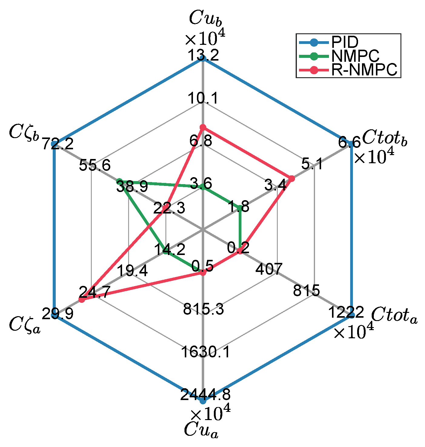
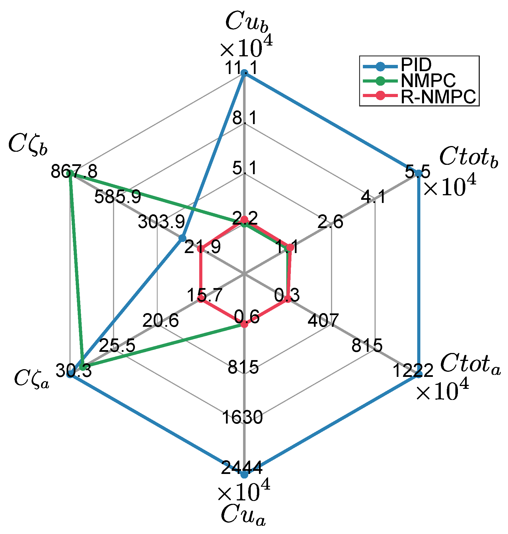
| Performance Metrics | PID | NMPC | % | R-NMPC | % |
|---|---|---|---|---|---|
| Metrics for the mobile base: | |||||
| Cum. Tracking error () | 7.33 × 101 | 3.06 × 101 | −58.2% | 2.46 × 101 | −66.4% |
| Cum. Control effort () | 51.14 × 10² | 32.60 × 10² | −36.2% | 41.45 × 10² | −18.9% |
| Total cost () | 51.87 × 10² | 32.91 × 10² | −36.5% | 41.69 × 10² | −19.6% |
| Metrics for the robot arm: | |||||
| Cum. Tracking error () | 8.80 × 101 | 7.51 × 101 | −14.6% | 5.07 × 101 | −42.3% |
| Cum. Control effort () | 31.55 × 10² | 33.28 × 10² | 5.4% | 37.16 × 10² | 17.7% |
| Total cost () | 32.43 × 10² | 34.03 × 10² | 4.9% | 37.66 × 10² | 16.12% |
| Performance Metrics | PID | NMPC | % | R-NMPC | % |
|---|---|---|---|---|---|
| Metrics for the mobile base: | |||||
| Cum. Tracking error () | 16.26 × 101 | 8.21 × 101 | −49.5% | 3.33 × 101 | −79.5% |
| Cum. Control effort () | 44.68 × 10² | 46.77 × 10² | 4.7% | 56.07 × 10² | 25.5% |
| Total cost () | 46.30 × 10² | 47.59 × 10² | 2.8% | 56.40 × 10² | 21.8% |
| Metrics for the robot arm: | |||||
| Cum. Tracking error () | 20.04 × 101 | 11.34 × 101 | −43.4% | 10.85 × 101 | −42.3% |
| Cum. Control effort () | 59.77 × 10² | 64.99 × 10² | 8.7% | 61.74 × 10² | 3.3% |
| Total cost () | 61.77 × 10² | 66.12 × 10² | 7.0% | 62.83 × 10² | 1.7% |
Disclaimer/Publisher’s Note: The statements, opinions and data contained in all publications are solely those of the individual author(s) and contributor(s) and not of MDPI and/or the editor(s). MDPI and/or the editor(s) disclaim responsibility for any injury to people or property resulting from any ideas, methods, instructions or products referred to in the content. |
© 2024 by the authors. Licensee MDPI, Basel, Switzerland. This article is an open access article distributed under the terms and conditions of the Creative Commons Attribution (CC BY) license (https://creativecommons.org/licenses/by/4.0/).
Share and Cite
Aro, K.; Guevara, L.; Torres-Torriti, M.; Torres, F.; Prado, A. Robust Nonlinear Model Predictive Control for the Trajectory Tracking of Skid-Steer Mobile Manipulators with Wheel–Ground Interactions. Robotics 2024, 13, 171. https://doi.org/10.3390/robotics13120171
Aro K, Guevara L, Torres-Torriti M, Torres F, Prado A. Robust Nonlinear Model Predictive Control for the Trajectory Tracking of Skid-Steer Mobile Manipulators with Wheel–Ground Interactions. Robotics. 2024; 13(12):171. https://doi.org/10.3390/robotics13120171
Chicago/Turabian StyleAro, Katherine, Leonardo Guevara, Miguel Torres-Torriti, Felipe Torres, and Alvaro Prado. 2024. "Robust Nonlinear Model Predictive Control for the Trajectory Tracking of Skid-Steer Mobile Manipulators with Wheel–Ground Interactions" Robotics 13, no. 12: 171. https://doi.org/10.3390/robotics13120171
APA StyleAro, K., Guevara, L., Torres-Torriti, M., Torres, F., & Prado, A. (2024). Robust Nonlinear Model Predictive Control for the Trajectory Tracking of Skid-Steer Mobile Manipulators with Wheel–Ground Interactions. Robotics, 13(12), 171. https://doi.org/10.3390/robotics13120171